Transient Analysis of a Selective Partial-Update LMS Algorithm

Abstract

In applications where large-order filters are needed, the computational load of adaptive filtering algorithms can become prohibitively expensive. In this paper, a comprehensive analysis of a selective partial-update least mean squares, named SPU-LMS-M-min, is developed. By employing the partial-update strategy for a non-normalized adaptive scheme, the designer can choose an appropriate number of update blocks considering a trade-off between convergence rate and computational complexity, which can result in a more than 40% reduction in the number of multiplications in some configurations compared to the traditional LMS algorithm. Based on the principle of minimum distortion, a selection criterion is proposed that is based on the input signal’s blocks with the lowest energy, whereas typical Selective Partial Update (SPU) algorithms use a selection criterion based on blocks with highest energy. Stochastic models are developed for the mean weights and mean and mean squared behaviour of the proposed algorithm, which are further extended to accommodate scenarios involving time-varying dynamics and suboptimal filter lengths. Simulation results show that the theoretical predictions are in good agreement with the experimental outcomes. Furthermore, it is demonstrated that the proposed selection criterion can be easily extended to active noise cancellation algorithms as well as algorithms utilizing variable filter length. This allows for the reduction of computational costs for these algorithms without compromising their asymptotic performance.

1. Introduction

Digital communications have seen rapid development, largely due to research in adaptive signal processing [1]. Other important applications of such techniques are system identification, acoustic and network echo cancelers, among others [2,3]. Especially in acoustic and channel equalization scenarios, the use of high-order adaptive filter is necessary. Thus, the required computational complexity can become the bottleneck in obtaining the expected performance [1]. In this context, strategies that reduce the computational load of adaptive filtering schemes are of great interest.

The ability of adaptive filters to adjust to variations in the environment in which they operate is what gives them flexibility and sophistication. The LMS algorithm is the most popular adaptive filtering approach. In general terms, it implements an online estimator that employs the observable data pair $\left\{\mathit{x}\right(k),d(k\left)\right\}$, where $d\left(k\right)\in \mathbb{R}$ is the reference signal and $\mathit{x}\left(k\right)\in {\mathbb{R}}^N$ denotes the input vector, defined as:

$$\mathit{x}\left(k\right)\triangleq {\left[\begin{array}{cccc}x\left(k\right)& x(k-1)& \dots & x(k-N+1)\end{array}\right]}^T.$$

(1)

where N denotes the filter length.

The LMS belongs to the class of supervised adaptive algorithms whose learning dynamics is driven by a feedback mechanism based on the error signal

$$e\left(k\right)\triangleq d\left(k\right)-{\mathit{w}}^T\left(k\right)\mathit{x}\left(k\right),$$

(2)

where $y\left(k\right)\triangleq {\mathit{w}}^T\left(k\right)\mathit{x}\left(k\right)$ is the filter output at the k-th iteration and $\mathit{w}\left(k\right)\in {\mathbb{R}}^N$ contains the N adaptive coefficients $\{w_0\left(k\right),w_1\left(k\right),\dots ,w_{N-1}\left(k\right)\}$. Moreover, the LMS update equation is traditionally derived from the stochastic gradient of the mean squared error, thereby yielding

$$\mathit{w}(k+1)=\mathit{w}\left(k\right)+\beta \mathit{x}\left(k\right)e\left(k\right),$$

(3)

where $\beta \in {\mathbb{R}}_{+}$ is the step size, whose choice implies a trade-off between asymptotic performance and convergence rate [4].

In a system identification task, the block diagram of the adaptive filter functioning is depicted in Figure 1, where the desired signal $d\left(k\right)$ sometimes is acquired by ingenious ways and signal $\nu \left(k\right)$ models the impact of inaccuracies in the measurement process, such as quantization noise.

Although the LMS is one of the simplest adaptive filtering algorithms, its update equation requires computational complexity proportional to the length of the adaptive coefficient vector $\mathit{w}\left(k\right)\in {\mathbb{R}}^N$ (see Equations (2) and (3)). Unfortunately, as already discussed, long transfer functions that occur in important real applications might demand a prohibitively large computational effort. Several schemes have been presented in the open literature to address this issue, such as sign-error, sign-data, and selective partial-update (SPU) strategies [5,6,7,8,9]. The latter schemes are the focus of this paper. The SPU-NLMS algorithm, one of the most popular SPU-based adaptive algorithms, is typically presented as a solution of a deterministic optimization problem [10]. The resulting update equation implies a reduced computational burden by decreasing the amount of tap modifications at every iteration. Concisely, the SPU-NLMS groups a set of adaptive coefficients in a single or multiple blocks, and selects the significant excitation data blocks according to their squared Euclidean norms. By a proper selection of input data blocks, the reduction of the computational burden can be attained.

In this paper, a new deterministic optimization approach is proposed, which avoids the normalization steps commonly required by SPU-based schemes. Based on it, a novel SPU-based LMS algorithm, referred to as SPU-LMS-M-min, is introduced. Furthermore, stochastic models are advanced to predict its mean weight dynamics and mean square error performance. In order to obtain a comprehensive analytic characterization of the learning abilities of the SPU-LMS-M-min algorithm, tracking and deficient-length analyses were also carried out.

The proposed coefficient selection method can be easily adapted to mitigate the computational cost of other strategies. For instance, Variable Filter-Length (VFL) algorithms [11,12,13,14,15,16] dynamically update the filter size throughout iterations, thereby reducing computational cost during transients. However, such algorithms update all adaptive coefficients, leading to an increased computational cost, especially in steady-state conditions. Additionally, these algorithms commonly asymptotically demand a longer filter length than optimal [17], implying unnecessary computational overhead. Both drawbacks can be alleviated through coefficient selection techniques. Thus, it is possible to reduce the computational cost of these algorithms without compromising their asymptotic performance, albeit with a controllable loss (to be judiciously chosen based on the application requirements) in convergence rate.

This paper is organized as follows. In Section 2, the proposed framework is derived, covering the single-block case for didactic purposes. A generalized algorithm that engenders a selection of several blocks in each update is the focus of Section 2.2. Section 3.1 introduces concepts for first-order analysis, which precedes the second-order analysis described at Section 3.2. Generalizations of the advanced stochastic model for both time-variant and deficient-length scenario approaches are presented on Section 3.3 and Section 3.4, respectively. Section 4 presents extensions of the proposed selection methodology to variable tap length and active noise cancellation (ANC) algorithms. Results and discussion are the focus of Section 5. At last, Section 6 contains the final considerations of the paper.

2. Proposed SPU-LMS-M-Min for a Single Block

Consider the following partition of the input vector $\mathit{x}\left(k\right)$ and the adaptive weights vector $\mathit{w}\left(k\right)$ into M equal-length blocks:

$$\mathit{x}\left(k\right)={\left[\begin{array}{cccc}{\mathit{x}}_0^T\left(k\right)& {\mathit{x}}_1^T\left(k\right)& \dots & {\mathit{x}}_{M-1}^T\left(k\right)\end{array}\right]}^T,$$

(4)

$$\mathit{w}\left(k\right)={\left[\begin{array}{cccc}{\mathit{w}}_0^T\left(k\right)& {\mathit{w}}_1^T\left(k\right)& \dots & {\mathit{w}}_{M-1}^T\left(k\right)\end{array}\right]}^T,$$

(5)

where the vectors ${\mathit{x}}_i\left(k\right)$ and ${\mathit{w}}_i\left(k\right)$ contains $N/M=L\in \mathbb{N}$ coefficients (For simplicity, L is supposed to be an integer number.) (for $i\in \{0,1,\dots ,M-1\}$). In order to reduce the computational burden, under the selective partial-update paradigm, only B blocks (for $B\in \{1,2,\dots ,M\}$) of the adaptive weights are updated in each iteration. For the sake of simplicity, in this section it is assumed that only one block is updated in each iteration (i.e., $B=1$). Note that for the existence of a block algorithm, it is necessary that $M>1$. Therefore, as $L=N/M$, we have $N>L$, an inequality valid for any value of B (including $B=1$).

Consider that the index of the block that will be updated (${\mathit{w}}_i\left(k\right)$) is denoted by i (later, the proposed selection procedure of such a index will be derived). The advanced SPU-LMS-M-min algorithm is the resulting solution of the following optimization problem:

$$\underset{{\mathit{w}}_i(k+1)}{min}\frac{1}{2}{\parallel {\mathit{w}}_i(k+1)-{\mathit{w}}_i\left(k\right)\parallel }^2\mathrm{s}.\mathrm{t}.e_p\left(k\right)=\left(1-\beta L{\sigma }_x^2\right)e\left(k\right),$$

(6)

where ${\sigma }_x^2$ denotes the variance in $x\left(k\right)$, and the posterior error $e_{\mathrm{p}}\left(k\right)$ is

$$\begin{array}{ccc}\hfill e_{\mathrm{p}}\left(k\right)& =& d\left(k\right)-{\mathit{w}}^T(k+1)\mathit{x}\left(k\right)\hfill \\ & =& d\left(k\right)-\left[{\mathit{w}}_i^T(k+1){\mathit{x}}_i\left(k\right)+{\overline{\mathit{w}}}_i^T(k+1){\overline{\mathit{x}}}_i\left(k\right)\right],\hfill \end{array}$$

(7)

where ${\overline{\mathit{w}}}_i\left(k\right)$ and ${\overline{\mathit{x}}}_i\left(k\right)$ are the vectors obtained by removing ${\mathit{w}}_i\left(k\right)$ and ${\mathit{x}}_i\left(k\right)$ from $\mathit{w}\left(k\right)$ and $\mathit{x}\left(k\right)$, respectively. The equality in Equation (6) imposes a linear constraint on the solution $\mathit{w}(k+1)$, which requires that the a posteriori error (dependent on the solution $\mathit{w}(k+1)$) be a fraction of the a priori error $e\left(k\right)$.

Using the Lagrange multipliers technique, the constrained optimization problem (6) can be translated into the following unconstrained one:

$${\mathcal{F}}_i\left[{\mathit{w}}_i(k+1)\right]=\frac{1}{2}{\parallel {\mathit{w}}_i(k+1)-{\mathit{w}}_i\left(k\right)\parallel }^2+\lambda \left[e_p\left(k\right)-\left(1-\beta L{\sigma }_x^2\right)e\left(k\right)\right],$$

(8)

where $\lambda \in \mathbb{R}$ is the Lagrange multiplier. Zeroing ${\nabla }_{{\mathit{w}}_i(k+1)}{\mathcal{F}}_i\left[{\mathit{w}}_i(k+1)\right]$ and using the approximation $L{\sigma }_x^2\approx {\parallel {\mathit{x}}_i\left(k\right)\parallel }^2,\forall i\in \{0,1,\dots ,M-1\}$, yields

$${\mathit{w}}_i(k+1)={\mathit{w}}_i\left(k\right)+\beta {\mathit{x}}_i\left(k\right)e\left(k\right),$$

(9)

whereas the remaining blocks are supposed to be unaltered, that is,

$${\overline{\mathit{w}}}_i(k+1)={\overline{\mathit{w}}}_i\left(k\right).$$

(10)

Remark 1.

It is worth mentioning that the approximation $L{\sigma }_x^2\approx \parallel {\mathit{x}}_i\left(k\right){\parallel }^2,\forall i\in \{0,1,\dots ,$$M-1\}$ is a feature of the proposed non-normalized SPU scheme, which is not necessary when normalized adaptive filtering algorithms are adopted. For long filters, exactly where one intends to reduce the computational complexity of adaptive filtering algorithms, such an approximation is less critical (assuming a stationary input signal). In the case of non-stationary signals, real-time estimation of the input signal variance can be achieved with a minor increase in computational complexity. However, in instances of highly non-stationary input signals, the efficacy of such a mechanism may be significantly compromised.

Note that Equation (9) represents the update equation after the selection of the block index i that will be updated, and that, indeed the adopted approximation makes the estimation of the variance in $x\left(k\right)$ unnecessary. The choice of such an index i can be oriented by the minimum distortion principle (MDP) [10]:

$$\begin{array}{ccc}\hfill i& =& \arg \underset{1\le j\le M}{min}{\parallel {\mathit{w}}_j(k+1)-{\mathit{w}}_j\left(k\right)\parallel }^2\hfill \\ & =& \arg \underset{1\le j\le M}{min}\parallel \beta {\mathit{x}}_j{\left(k\right)e\left(k\right)\parallel }^2=\arg \underset{1\le j\le M}{min}{\parallel {\mathit{x}}_j\left(k\right)\parallel }^2,\hfill \end{array}$$

(11)

so that the update equation of the advanced SPU-LMS-M-min algorithm can be written as

$${\mathit{w}}_i(k+1)={\mathit{w}}_i\left(k\right)+\beta {\mathit{x}}_i\left(k\right)e\left(k\right),i=\arg \underset{0\le j\le M-1}{min}{\parallel {\mathit{x}}_j\left(k\right)\parallel }^2.$$

(12)

Remark 2.

Observe that the advanced criterion selects a block whose quadratic norm is the smallest among all blocks, whereas in established algorithms, the block with the largest norm is chosen [10]. For example, the selection procedure of the M-max LMS chooses the block whose ${\mathsf{\ell }}_2$-norm is the largest. This difference derives from the fact that in this paper, the derivation procedure relies on a deterministic and local problem induced by the minimum distortion principle, whereas normally, the stochastic-gradient interpretation of the LMS algorithm is adopted in order to motivate the derivation of SPU-based non-normalized algorithms.

2.1. Computational Complexity

In order to guarantee an effective reduction of the computational burden, the selection of index i required by the SPU-LMS-M-min algorithm (see Equation (12)) should be carried out by fast algorithms for running ordering and max/min calculation criteria [18]. Assuming the adoption of efficient ordering algorithms (which do not require neither multiplications nor sums, but only comparisons between numbers), it is possible to evaluate the number of additions and multiplications required per iteration by the SPU-LMS-M-min.

Table 1. Number of multiplications, additions, comparisons (i.e., if one value is greater than another, required to find the maximum or minimum value of a vector), and divisions at each iteration of the algorithms and their respective selective partial update variants [10,19]. S denotes the period of coefficient updates (i.e., it is assumed that updates occur only every S consecutive input vectors).

Algorithm	Multiplication	Addition	Comparison	Division
LMS-Based
Standard	2N + 1	2N	−	−
M-min	N + $BL$ + 1	N + $BL$	2[$lo{g}_{2}N]$ + 2	−
Periodic	N + (N + 1)/S	N + N/S	−	−
Sequential	N + $BL$ + 1	N + $BL$	−	−
Stochastic	N + $BL$ + 3	N + $BL$ + 2	−	−
M-max	N + $BL$ + 1	N + $BL$	2[$lo{g}_{2}N]$ + 2	−
Norm. Selective	N + $BL$ + 2	N + $BL$ + 2	2[$lo{g}_{2}N]$ + 2	1

compares the computational complexity of the elements of an LMS algorithm bundle, taking into account SPU-NLMS (Norm. selective) and LMS-SPU-M-(max|min). It is noteworthy that update Equation (12) requires $N+BL+1$ multiplications, whereas the standard LMS requires $2N+1$ multiplications per iteration. Since the designer might enforce the condition $BL<N$, a significant reduction in computational burden requirement can be attained. For example, for a configuration with $N=4000$, $M=8$ and $B=1$, the number of required multiplications per iteration is reduced by 43.65%. Furthermore, no divisions are required, which is an advantage of the proposed non-normalized scheme. It is noteworthy that such complexity reduction may decrease the convergence rate of the adaptive algorithm, which may not be feasible in applications imposing stringent criteria on the number of iterations required for the learning process to reach a steady state.

After the following new derivation approach of the target algorithm SPU-LMS-M-min, it is expected that presents some distinct features, such as reduction in the convergence rate, which can be predicted and elucidated by stochastic models. Some models based on conventional assumptions are described in the following sections. Note that such theoretical analysis are appreciated in the open literature due to their ability to provide performance guarantees for the algorithm designer, as well as important insights about its functioning.

2.2. SPU-LMS-M-Min for Multiple Blocks

The ensuing derivations facilitates the understanding of the generalized formulation of the algorithm, in which the designer intends to update B blocks in each iteration. Consider these indexes are denoted by ${\mathcal{I}}_B=\{i_0,i_1,\dots ,i_{B-1}\}$. Equation (8) can be extended by the following generalized optimization problem:

$$\underset{{\mathit{w}}_{{\mathcal{I}}_B}(k+1)}{min}\frac{1}{2}{\parallel {\mathit{w}}_{{\mathcal{I}}_B}(k+1)-{\mathit{w}}_{{\mathcal{I}}_B}\left(k\right)\parallel }^2$$

$$\mathrm{s}.\mathrm{t}.e_p\left(k\right)=\left(1-\beta B\frac{N}{M}{\sigma }_x^2\right)e\left(k\right),$$

(13)

where ${\mathit{w}}_{{\mathcal{I}}_B}(k+1)\triangleq {\left[\begin{array}{cccc}{\mathit{w}}_{i_0}^T\left(k\right)& {\mathit{w}}_{i_1}^T\left(k\right)& \dots & {\mathit{w}}_{i_{B-1}}^T\left(k\right)\end{array}\right]}^T$.

Using similar steps to those in (9), one may describe the SPU-LMS-M-min algorithm that updates B blocks by

$${\mathit{w}}_{{\mathcal{I}}_B}(k+1)={\mathit{w}}_{{\mathcal{I}}_B}\left(k\right)+\beta {\mathit{x}}_{{\mathcal{I}}_B}\left(k\right)e\left(k\right),$$

(14)

where ${\mathcal{I}}_B$ can be computed by the following rule:

$$\begin{array}{ccc}\hfill {\mathcal{I}}_B& =& \arg \underset{J_B\in S}{min}{\parallel {\mathit{w}}_{J_B}(k+1)-{\mathit{w}}_{J_B}\left(k\right)\parallel }^2\hfill \\ & =& \arg \underset{J_B\in S}{min}\parallel \beta {\mathit{x}}_{J_B}{\left(k\right)e\left(k\right)\parallel }^2=\arg \underset{J_B\in S}{min}{\parallel {\mathit{x}}_{J_B}\left(k\right)\parallel }^2\hfill \\ & =& \arg \underset{J_B\in S}{min}\sum _{j\in J_B}{\parallel {\mathit{x}}_j\left(k\right)\parallel }^2.\hfill \end{array}$$

(15)

3. Stochastic Modelling of the Proposed Algorithm

3.1. First-Order Analysis

Note that Equation (12) can be rewritten as

$$\mathit{w}(k+1)=\mathit{w}\left(k\right)+\beta \mathsf{\Gamma }\left(k\right)\mathit{x}\left(k\right)e\left(k\right),$$

(16)

where $\mathsf{\Gamma }\left(k\right)$ is an $N\times N$ diagonal matrix, with each element of its main diagonal denoted as ${\gamma }_i\left(k\right)$, where i is the associated block index. The main diagonal elements of $\mathsf{\Gamma }\left(k\right)$ are obtained by

$${\gamma }_i\left(k\right)=\left\{\begin{array}{cc}0,& \mathrm{if}i\notin {\mathcal{I}}_B\hfill \\ 1,& \mathrm{if}i\in {\mathcal{I}}_B\hfill \end{array}\right..$$

(17)

Consider that reference signal $d\left(k\right)$ is generated by the following affine regression model:

$$d\left(k\right)={\left[{\mathit{w}}^{★}\right]}^T\mathit{x}\left(k\right)+\nu \left(k\right),$$

(18)

where ${\mathit{w}}^{★}\in {\mathbb{R}}^N$ is a vector that contains the coefficients of the ideal (and unknown) plant and $\nu \left(k\right)$ is an additive noise. Defining the deviation coefficient vector as $\tilde{\mathit{w}}\left(k\right)\triangleq {\mathit{w}}^{★}-\mathit{w}\left(k\right)$, the following recursion can be obtained from Equation (16):

$$\tilde{\mathit{w}}(k+1)=\left(\mathit{I}-\beta \mathsf{\Gamma }\left(k\right)\mathit{x}\left(k\right){\mathit{x}}^T\left(k\right)\right)\tilde{\mathit{w}}\left(k\right)-\beta \mathsf{\Gamma }\left(k\right)\mathit{x}\left(k\right)\nu \left(k\right),$$

(19)

which is a non-homogeneous stochastic difference equation, where $-\beta \mathsf{\Gamma }\left(k\right)\mathit{x}\left(k\right)\nu \left(k\right)$ acts as a driving force that avoids the asymptotic convergence of the deviation vector energy to zero. A first-order stochastic analysis of the SPU-LMS-M-min algorithm can be performed by applying the expectation operator in $\mathbb{E}\left[·\right]$ in (19), which leads (using the popular independence assumption-IA  [4]) to

$$\mathbb{E}\left[\tilde{\mathit{w}}(k+1)\right]=\left(\mathit{I}-\beta {\mathit{R}}_{\mathsf{\Gamma }}\right)\mathbb{E}\left[\tilde{\mathit{w}}\left(k\right)\right],$$

(20)

where ${\mathit{R}}_{\mathsf{\Gamma }}\triangleq \mathbb{E}\left[\mathsf{\Gamma }\left(k\right)\mathit{x}\left(k\right){\mathit{x}}^T\left(k\right)\right]$.

Remark 3.

Note that Equation (20) implies that the SPU-LMS-M-min, under a sufficient excitation condition, performs an asymptotically unbiased estimation [20]. Furthermore, the maximum step size that guarantees mean-weight convergence can be obtained by assuming

$$\beta <\frac{2}{\rho \left[{\mathit{R}}_{\mathsf{\Gamma }}\right]},$$

(21)

where $\rho \left[{\mathit{R}}_{\mathsf{\Gamma }}\right]$ denotes the spectral radius of ${\mathit{R}}_{\mathsf{\Gamma }}$, i.e., $\rho \left[{\mathit{R}}_{\mathsf{\Gamma }}\right]\triangleq {max}_i\left|{\lambda }_i\left({\mathit{R}}_{\mathsf{\Gamma }}\right)\right|$, where ${\lambda }_i$ is the i-th eigenvalue of ${\mathit{R}}_{\mathsf{\Gamma }}$. Unfortunately, a stable-in-the-mean adaptive filter may perform an estimation with unbounded variance, so that a second-order stochastic analysis is necessary in order to achieve proper performance guarantees [20]. In the derivation of Equation (20), the statistically strong (but physically plausible) assumption that the additive noise is white and statistically independent from the remaining random variables is employed. Such a noise assumption (NA) is almost ubiquitous and is utilized henceforth.

3.2. Second-Order Analysis

The usage of the independence assumption implies that the expectation value of the matrix

$$\mathsf{\Phi }\left(k\right)=\tilde{\mathit{w}}\left(k\right){\tilde{\mathit{w}}}^T\left(k\right)$$

(22)

has a major rule in a second-order stochastic model of adaptive algorithms [20]. Using Equation (19), a recursion for $\mathsf{\Phi }\left(k\right)$ can be obtained as

$$\begin{array}{ccc}\hfill \mathsf{\Phi }(k+1)& =& \mathsf{\Phi }\left(k\right)-\beta \mathsf{\Phi }\left(k\right)\mathit{x}\left(k\right){\mathit{x}}^T\left(k\right)\mathsf{\Gamma }\left(k\right)\hfill \\ & & -\beta \mathsf{\Gamma }\left(k\right)\mathit{x}\left(k\right){\mathit{x}}^T\left(k\right)\mathsf{\Phi }\left(k\right)\hfill \\ & & +{\beta }^2\mathsf{\Gamma }\left(k\right)\mathit{x}\left(k\right){\mathit{x}}^T\left(k\right)\mathsf{\Phi }\left(k\right)\mathit{x}\left(k\right){\mathit{x}}^T\left(k\right)\mathsf{\Gamma }\left(k\right)\hfill \\ & & +{\beta }^2{\nu }^2\left(k\right)\mathsf{\Gamma }\left(k\right)\mathit{x}\left(k\right){\mathit{x}}^T\left(k\right)\mathsf{\Gamma }\left(k\right)+\mathcal{O}\left[\nu \left(k\right)\right],\hfill \end{array}$$

(23)

where $\mathcal{O}\left[\nu \right(k\left)\right]$ contains first-order noise components, which are irrelevant to the following analysis.

Recursion (23) can be rewritten in a more adequate formulation by applying the relationship

$$\mathrm{vec}\left(\mathit{XYZ}\right)=\left({\mathit{Z}}^T\otimes \mathit{X}\right)\mathrm{vec}\left(\mathit{Y}\right),$$

(24)

where $\mathrm{vec}\left(\mathit{A}\right)$ is an operator that stacks the columns of matrix $\mathit{A}$ in order to generate a column-type vector and ⊗ denotes the Kronecker product. Employing such a formulation, applying the expectation operator and using the independence assumption, leads to the following time-invariant state space equation:

$$\mathit{v}(k+1)=\mathit{A}\mathit{v}\left(k\right)+\mathit{b},$$

(25)

where

$$\mathit{v}\left(k\right)\triangleq \mathbb{E}\left\{\mathrm{vec}\left[\mathsf{\Phi }\left(k\right)\right]\right\},$$

(26)

$$\begin{array}{ccc}\hfill \mathit{A}& \triangleq & \mathit{I}-\beta \mathbb{E}\left\{\left[\mathsf{\Gamma }\left(k\right)\mathit{x}\left(k\right){\mathit{x}}^T\left(k\right)\right]\otimes \mathit{I}\right\}\hfill \\ & & -\beta \mathbb{E}\left\{\mathit{I}\otimes \left[\mathsf{\Gamma }\left(k\right)\mathit{x}\left(k\right){\mathit{x}}^T\left(k\right)\right]\right\}\hfill \\ & & +{\beta }^2\mathbb{E}\left\{\left[\mathsf{\Gamma }\left(k\right)\mathit{x}\left(k\right){\mathit{x}}^T\left(k\right)\right]\otimes \left[\mathsf{\Gamma }\left(k\right)\mathit{x}\left(k\right){\mathit{x}}^T\left(k\right)\right]\right\},\hfill \end{array}$$

(27)

and

$$\mathit{b}\triangleq {\beta }^2{\sigma }_{\nu }^2\mathbb{E}\left\{\mathrm{vec}\left[\mathsf{\Gamma }\left(k\right)\mathit{x}\left(k\right){\mathit{x}}^T\left(k\right)\mathsf{\Gamma }\left(k\right)\right]\right\},$$

(28)

where ${\sigma }_{\nu }^2$ is the variance of the additive noise.

Since $\mathrm{vec}\left[\mathit{X}\right]$ is a bijection operator, all information of the mismatch covariance matrix ${\mathit{R}}_{\tilde{\mathit{w}}}\left(k\right)\triangleq \mathbb{E}\left[\mathsf{\Phi }\left(k\right)\right]$ can be extracted from $\mathit{v}\left(k\right)$. From both IA and NA stochastic hypotheses, the mean square deviation (MSD) and mean square error (MSE) performance metrics can be predicted for the k-th iteration using [20]

$$\begin{array}{ccc}\hfill \mathrm{MSD}\left(k\right)& \triangleq & \mathbb{E}\left[\parallel {\mathit{w}}^{★}{-\mathit{w}\left(k\right)\parallel }^2\right]\approx \mathrm{Tr}\left[{\mathit{R}}_{\tilde{\mathit{w}}}\left(k\right)\right],\hfill \end{array}$$

(29)

$$\begin{array}{ccc}\hfill \mathrm{MSE}\left(k\right)& \triangleq & \mathbb{E}\left[e^2\left(k\right)\right]\approx {\sigma }_{\nu }^2+\mathrm{Tr}\left[{\mathit{R}}_{\mathit{x}}{\mathit{R}}_{\tilde{\mathit{w}}}\left(k\right)\right],\hfill \end{array}$$

(30)

where $\mathrm{Tr}\left[\mathit{Y}\right]$ denotes the trace of matrix $\mathit{Y}$ and ${\mathit{R}}_{\mathit{x}}\triangleq \mathbb{E}\left[\mathit{x}\left(k\right){\mathit{x}}^T\left(k\right)\right]$ is the input autocorrelation matrix.

Remark 4.

It is noteworthy that Equation (25) is able to yield a closed-form estimate for both asymptotic MSD and MSE, provided the algorithm is stable. In this case, the steady-state vector ${\mathit{v}}_{\infty }\triangleq {lim}_{k\to \infty }\mathit{v}\left(k\right)$ can be computed by [20]

$${\mathit{v}}_{\infty }={\left(\mathit{I}-\mathit{A}\right)}^{-1}\mathit{b}.$$

(31)

3.3. Tracking Analysis

Since adaptive filters that present good performance in stationary environments do not necessarily exhibit good learning behavior in the identification of time-variant plants [21], obtaining a stochastic model that offers guarantees with respect to the algorithm learning capabilities in a tracking scenario is crucial.

A popular model that accounts for temporal variation in ${\mathit{w}}^{★}\left(k\right)$ can be described as a first-order Markov process [22]

$${\mathit{w}}^{★}(k+1)={\mathit{w}}^{★}\left(k\right)+\mathit{q}\left(k\right),$$

(32)

where the statistical characterization of the perturbation vector $\mathit{q}\left(k\right)$ is established by the assumption stated below.

Assumption A1.

Tracking assumption(TA): vector $\mathit{q}\left(k_1\right)$ is statistically independent from the input data and from $\mathit{q}\left(k_2\right)$, $\forall k_2\ne k_1$. Furthermore, its autocorrelation matrix is given by ${\mathit{R}}_q\triangleq \mathbb{E}\left[\mathit{q}\left(k\right){\mathit{q}}^T\left(k\right)\right]{\sigma }_q^2{\mathit{I}}_N$, where ${\mathit{I}}_N$ denotes the N-order identity matrix.

In order to create coefficient error vector in a deviation form, let us consider Equation (32) compared to Equation (16):

$$\begin{array}{c}\hfill {\mathit{w}}^{★}(k+1)-\mathit{w}(k+1)={\mathit{w}}^{★}(k+1)-\mathit{w}\left(k\right)-\beta \mathsf{\Gamma }\left(k\right)\mathit{x}\left(k\right)e\left(k\right)\\ \hfill \tilde{\mathit{w}}(k+1)=\mathit{q}\left(k\right)+{\mathit{w}}^{★}\left(k\right)-\mathit{w}\left(k\right)-\beta \mathsf{\Gamma }\left(k\right)\mathit{x}\left(k\right)e\left(k\right)\\ \hfill \tilde{\mathit{w}}(k+1)=\tilde{\mathit{w}}\left(k\right)-\beta \mathsf{\Gamma }\left(k\right)\mathit{x}\left(k\right)e\left(k\right)+\mathit{q}\left(k\right),\end{array}$$

(33)

By also replacing $e\left(k\right)$ by Equation (2) at Equation (34), after some arrangements, the following recursion deviation vector $\tilde{\mathit{w}}\left(k\right)$ can be rewritten:

$$\begin{array}{c}\hfill \tilde{\mathit{w}}(k+1)=\left(\mathit{I}-\beta \mathsf{\Gamma }\left(k\right)\mathit{x}\left(k\right){\mathit{x}}^T\left(k\right)\right)\tilde{\mathit{w}}\left(k\right)-\\ \hfill -\beta \mathsf{\Gamma }\left(k\right)\mathit{x}\left(k\right)\nu \left(k\right)+\mathit{q}\left(k\right)\end{array}$$

(34)

In order to reach a mean-square performance model (following similar steps than those employed to obtain Equation (25)), taking into account Equation (34), which can be used to derive the non-homogeneous stochastic difference equation by performing the product between Equation (34) and its transposed version, reaching this equation:

$$\begin{array}{ccc}\hfill \mathsf{\Phi }(k+1)& =& \mathsf{\Phi }\left(k\right)-\beta \mathsf{\Phi }\left(k\right)\mathit{x}\left(k\right){\mathit{x}}^T\left(k\right)\mathsf{\Gamma }\left(k\right)\hfill \\ & & -\beta \mathsf{\Gamma }\left(k\right)\mathit{x}\left(k\right){\mathit{x}}^T\left(k\right)\mathsf{\Phi }\left(k\right)\hfill \\ & & +{\beta }^2\mathsf{\Gamma }\left(k\right)\mathit{x}\left(k\right){\mathit{x}}^T\left(k\right)\mathsf{\Phi }\left(k\right)\mathit{x}\left(k\right){\mathit{x}}^T\left(k\right)\mathsf{\Gamma }\left(k\right)\hfill \\ & & +{\beta }^2{\nu }^2\left(k\right)\mathsf{\Gamma }\left(k\right)\mathit{x}\left(k\right){\mathit{x}}^T\left(k\right)\mathsf{\Gamma }\left(k\right)\hfill \\ & & +\mathit{q}\left(k\right){\mathit{q}}^T\left(k\right)+\mathcal{O}\left[\nu \left(k\right)\right]+\mathcal{O}\left[q\left(k\right)\right],\hfill \end{array}$$

(35)

where $\mathsf{\Phi }\left(k\right)$ is as defined by Equation (22), $\mathcal{O}\left[\nu \right(k\left)\right]$ denotes noise-related terms that will not interfere with the hereinafter analysis, and $\mathcal{O}\left[q\right(k\left)\right]$ is related to the first-order perturbation vector, which would also not be part of that balance. Aiming to make the mathematics tractable, the application of the expectation operator from Equation (36) should be performed alongside some assumptions, which are described below.

$$\mathit{v}(k+1)=\mathit{A}\mathit{v}\left(k\right)+\mathit{b}+\mathit{c},$$

(36)

where $\mathit{c}\triangleq \mathbb{E}\left\{\mathrm{vec}\left[\mathit{q}\left(k\right){\mathit{q}}^T\left(k\right)\right]\right\}$.

Remark 5.

Note that under the considered tracking scenario, the stability region of the algorithm remains unaltered, since the time-invariant transition matrix $\mathit{A}$ is the same as the stationary configuration [20].

3.4. Deficient-Length Analysis

There are several practical situations to motivate that analysis: Usually we do not know in advance the transfer function to be identified, no how limited the computational resources would be. In addition, the length of the adaptive filter N is often less than the length L of the transfer function to be identified. In this deficient-length setting, according to [4], it is possible to model the transfer function coefficients vector and the reference signal as:

$${\mathit{w}}_{\mathit{o}}^{★}={[{\mathit{w}}^{★},{\overline{\mathit{w}}}^{★}]}^T,$$

(37)

$$d_{\mathrm{def}}\left(k\right)={\left[{\mathit{w}}^{★}\right]}^T\mathit{x}\left(k\right)+{\left[{\overline{\mathit{w}}}^{★}\right]}^T\overline{\mathit{x}}\left(k\right)+\nu \left(k\right),$$

(38)

where

$$\overline{\mathit{x}}\left(k\right)\triangleq \left[\begin{array}{cccc}x(k-N)& x(k-N-1)& \cdots & x(k-N-L+1)\end{array}\right]$$

(39)

and ${\overline{\mathit{w}}}^{★}\in {\mathbb{R}}^L$ is the L-length component of the ideal transfer function, ${\mathit{w}}^{★}$, whose total length is $N+L$, that the adaptive filter is not able to emulate. Considering Equation (2) and the previous definitions, it is possible to write $e_{\mathrm{def}}\left(k\right)$ in the deficient-length approach:

$$\begin{array}{ccc}\hfill e_{\mathrm{def}}\left(k\right)& & =d_{\mathrm{def}}\left(k\right)-{\tilde{\mathit{w}}}^T\left(k\right)\mathit{x}\left(k\right)\hfill \\ & & ={\left({\mathit{w}}^{★}\right)}^T\mathit{x}\left(k\right)+{\left({\overline{\mathit{w}}}^{★}\right)}^T\overline{\mathit{x}}\left(k\right)+\nu \left(k\right)-{\tilde{\mathit{w}}}^T\left(k\right)\mathit{x}\left(k\right)\hfill \\ & & ={\tilde{\mathit{w}}}^T\left(k\right)\mathit{x}\left(k\right)+{\left({\overline{\mathit{w}}}^{★}\right)}^T\overline{\mathit{x}}\left(k\right)+\nu \left(k\right),\hfill \end{array}$$

(40)

Subsequently, defining input, reference signals, and error, it is necessary to rewrite Equation (16) for the context of the deficient-length analysis with Equation (41):

$$\begin{array}{ccc}\hfill {\mathit{w}}^{★}(k+1)-\mathit{w}(k+1)& =& {\mathit{w}}^{★}(k+1)-\mathit{w}\left(k\right)-\beta \mathsf{\Gamma }\left(k\right)\mathit{x}\left(k\right)e_{\mathrm{def}}\left(k\right)\hfill \\ \hfill \tilde{\mathit{w}}(k+1)& =& \tilde{\mathit{w}}\left(k\right)-\beta \mathsf{\Gamma }\left(k\right)\mathit{x}\left(k\right)e_{\mathrm{def}}\left(k\right)\hfill \\ \hfill \tilde{\mathit{w}}(k+1)& =& \tilde{\mathit{w}}\left(k\right)-\beta \mathsf{\Gamma }\left(k\right)\mathit{x}\left(k\right)[{\tilde{\mathit{w}}}^T\left(k\right)\mathit{x}\left(k\right)\hfill \\ & +& {\left({\overline{\mathit{w}}}^{★}\right)}^T\overline{\mathit{x}}\left(k\right)+\nu \left(k\right)]\hfill \\ \hfill \tilde{\mathit{w}}(k+1)& =& \tilde{\mathit{w}}\left(k\right)-\beta \mathsf{\Gamma }\left(k\right)\mathit{x}\left(k\right){\mathit{x}}^T\left(k\right)\tilde{\mathit{w}}\left(k\right)\hfill \\ & -& \beta \mathsf{\Gamma }\left(k\right)\mathit{x}\left(k\right){\overline{\mathit{x}}}^T\left(k\right){\overline{\mathit{w}}}^{★}-\beta \mathsf{\Gamma }\left(k\right)\mathit{x}\left(k\right)\nu \left(k\right)\hfill \end{array}$$

(41)

Calculating the product between Equation (41) and its respective transposed version, applying the same steps as than those employed to obtain Equation (25), also to make more comprehensible the mathematics, the following assumption will be considered in the deficient-length setup:

Assumption A2.

Whiteness assumption (WA). The excitation data is white.

Remark 6.

Note that WA is a common assumption in the field of adaptive filtering analysis, even when the input signal is non-stationary (see, e.g., [23]). A more evolved analysis is necessary if such an assumption should be circumvented [24]. Using  WA and the previous assumptions, it can be demonstrated that in the suboptimal scenario (38) the vector $\mathit{v}\left(k\right)$ is updated according to

$$\begin{array}{c}\hfill {\mathit{v}}_{k+1}=\mathit{A}{\mathit{v}}_k+\mathit{b}+\mathit{d}\end{array}$$

(42)

where

$$\begin{array}{c}\hfill \mathit{d}\triangleq {\beta }^2\mathbb{E}\left\{\left[\mathsf{\Gamma }\left(k\right)\mathit{x}\left(k\right){\mathit{x}}^T\left(k\right)\right]\otimes \left[\mathsf{\Gamma }\left(k\right)\mathit{x}\left(k\right){\mathit{x}}^T\left(k\right)\right]\right\}\overline{\mathit{v}}\end{array}$$

(43)

and $\overline{\mathit{v}}\triangleq \mathit{vec}\left[\overline{\mathit{w}}{\overline{\mathit{w}}}^T\right]$.

4. Extensions of the Proposed Framework

Although the entire discussion up to this point has been focused on the LMS algorithm and the system identification problem, the proposed framework can be easily extended to VTL strategies and active noise cancellation (ANC) problems. This section details the extension of the proposed methodology for both cases. It is observed that the computational cost reduction capacity of the proposed methodology can be easily extended to other schemes and scenarios.

The computational complexity of an adaptive filter can be reduced through the use of VTL schemes [11,12,13,14,15,16], which adjust the tap length in real time. These algorithms share with the SPU technique the ability to present reduced computational cost during transients. However, under steady-state conditions, they update all filter coefficients. This, together with the tendency of these algorithms to overestimate the optimal steady-state adaptive filter length, can lead to excessively high steady-state computational costs [17]. Such an issue can be circumvented by using the proposed selection update scheme.

As a proof of concept, we consider the VTL algorithm proposed in [12]. The algorithm adjusts the pseudo fractional tap-length $n_{\mathrm{f}}\left(k\right)\in {\mathbb{R}}_{+}$ through the following updating rule:

$$n_f(k+1)=(n_f\left(k\right)-\alpha )-\gamma \left\{{\left[e^{\left(N\right(k\left)\right)}\left(k\right)\right]}^2-{\left[e^{\left(N\right(k)-\Delta )}\left(k\right)\right]}^2\right\},$$

(44)

where $\alpha$, $\gamma$, and $\Delta$ are adjustable parameters, the choice of which has been widely discussed in the literature (see, e.g., [17]), $N\left(k\right)$ is the length of the adaptive filter in the kth iteration, and $e^{\left(L\right)}\left(k\right)$ is the error calculated with a filter of length L. The algorithm adjusts the tap length using the rule:

$$N(k+1)=\left\{\begin{array}{cc}\lfloor n_{\mathrm{f}}\left(k\right)\rfloor ,& |N\left(k\right)-n_{\mathrm{f}}\left(k\right)|\ge \delta ,\hfill \\ N\left(k\right),& \mathrm{otherwise}\hfill \end{array}\right.,$$

(45)

where $\delta \in {\mathbb{R}}_{+}$ is also a tuning parameter. Since the size of the adaptive filter in VTL schemes varies dynamically, it is challenging to choose a block size M for an SPU technique insertion such that the current size of the adaptive filter is a multiple of M. To overcome this issue, we consider the choice $M=N\left(k\right)$. Thus, each sample of the input vector corresponds mathematically to a block of the SPU methodology. One can then choose B to ensure that a certain percentage of the adaptive coefficients in the VTL technique are updated in a given iteration, using the criterion proposed in Equation (15) for the coefficients to be updated. This ensures that the B adaptive coefficients to be updated are associated with the B samples of the input vector $\mathit{x}\left(k\right)$ with the lowest magnitudes. The resulting algorithm exhibits asymptotic performance equivalent to that of the original VTL algorithm, with lower computational cost. However, due to the coefficient selection, there is also a loss in convergence rate, which is inevitable when constraints on computational complexity are strict.

ANC algorithms can also benefit from adopting the coefficient selection strategy. Consider, for example, the Filtered-X LMS (FX-LMS) algorithm [15,25,26], whose block diagram is presented in Figure 2. The FX-LMS algorithm is used in active noise control applications to minimize noise in a primary input signal. It operates by subtracting the output of an adaptive filter from a reference signal, aiming to estimate and cancel unwanted noise in the primary input. The algorithm adjusts the adaptive filter coefficients iteratively using the LMS approach, with each update being proportional to the product of the error signal (the difference between the reference signal and the filtered input) and the input signal. The process continues iteratively until convergence, where the adaptive filter effectively minimizes the mean square error, resulting in reduced noise in the primary input signal. The filtering of the input signal is performed through an estimate $\widehat{S}\left(z\right)$ of the secondary path $S\left(z\right)$. The computational cost of the FX-LMS algorithm can be mitigated by selectively updating a fraction of its coefficients using the proposed criterion. Similar to the case of VTL techniques, a maintenance of the asymptotic performance of the FX-LMS algorithm is observed, along with a controllable loss in the convergence rate.

5. Results

In this section, simulation results are presented in order to assess the quality of theoretical predictions using simulated curves obtained through 1000 independent Monte Carlo trials (except when a different value is explained). In all of the following scenarios, the additive noise derives from a Gaussian and white process.

5.1. First-Order Analysis

In this scenario, the proposed model of the algorithm is evaluated with regard to the average evolution of the coefficients. The plant to be emulated consists of the first 64 coefficients from Model 4 of [27]. The total number of blocks is $M=8$. To evaluate the accuracy of the proposed model’s behavior, we consider a configuration in which the input signal is white Gaussian and of unitary variance. The SPU-LMS-M-min parameters are: $\beta ={10}^{-2}$, ${\sigma }_{\nu }^2={10}^{-6}$. The results shown in Figure 3 reveal good correspondence with the experimental results and confirm the expectation that an increase in B implies a faster convergence of the algorithm. It is important to point out that Figure 3a evaluates the evolution of the coefficient $w_8\left(k\right)$, among the 64 coefficients, while Figure 3b presents the evolution of the coefficient $w_{34}\left(k\right)$, among the 64 adaptive coefficients. In both figures, an almost perfect adherence can be seen, with updates of one, two, three, or four blocks. Such adherence allows us to verify that the first-order theoretical modeling is validated by the results obtained via simulation, indicating that the hypotheses described do not project significant discrepancies in relation to the real behavior of the algorithm in this scenario.

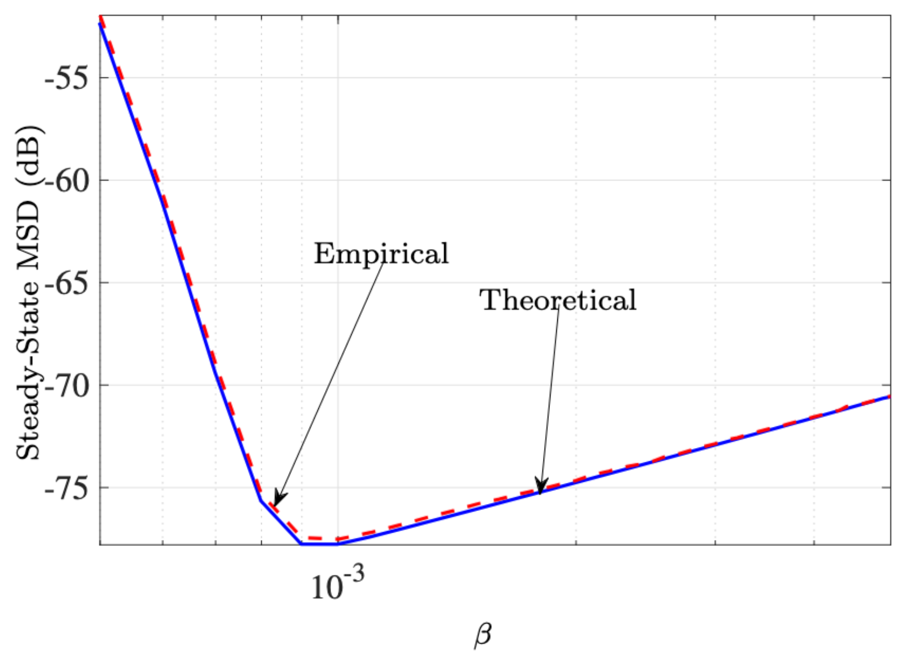
5.2. Second-Order Analysis

In this scenario, the proposed model of the algorithm is evaluated with respect to the MSD and MSE metrics. The plant to be emulated contains the first 32 coefficients from Model 4 of [27]. The total number of blocks is $M=8$. The input signal is white and the SPU-LMS-M-min parameters are: $\beta ={10}^{-2}$, ${\sigma }_{\nu }^2={10}^{-6}$. The results shown in Figure 4a reveal good correspondence between the theoretical and experimental curves of the MSD, both in steady-state and transient regimes. There is also confirmation that an increase in B implies a higher convergence rate of the algorithm. Such an increase also implies greater adherence between theoretical and experimental results (see the curve with $B=4$). The results shown in Figure 4b reveal good correspondence between the theoretical and experimental curves of the MSE, both in steady-state and transient regimes.

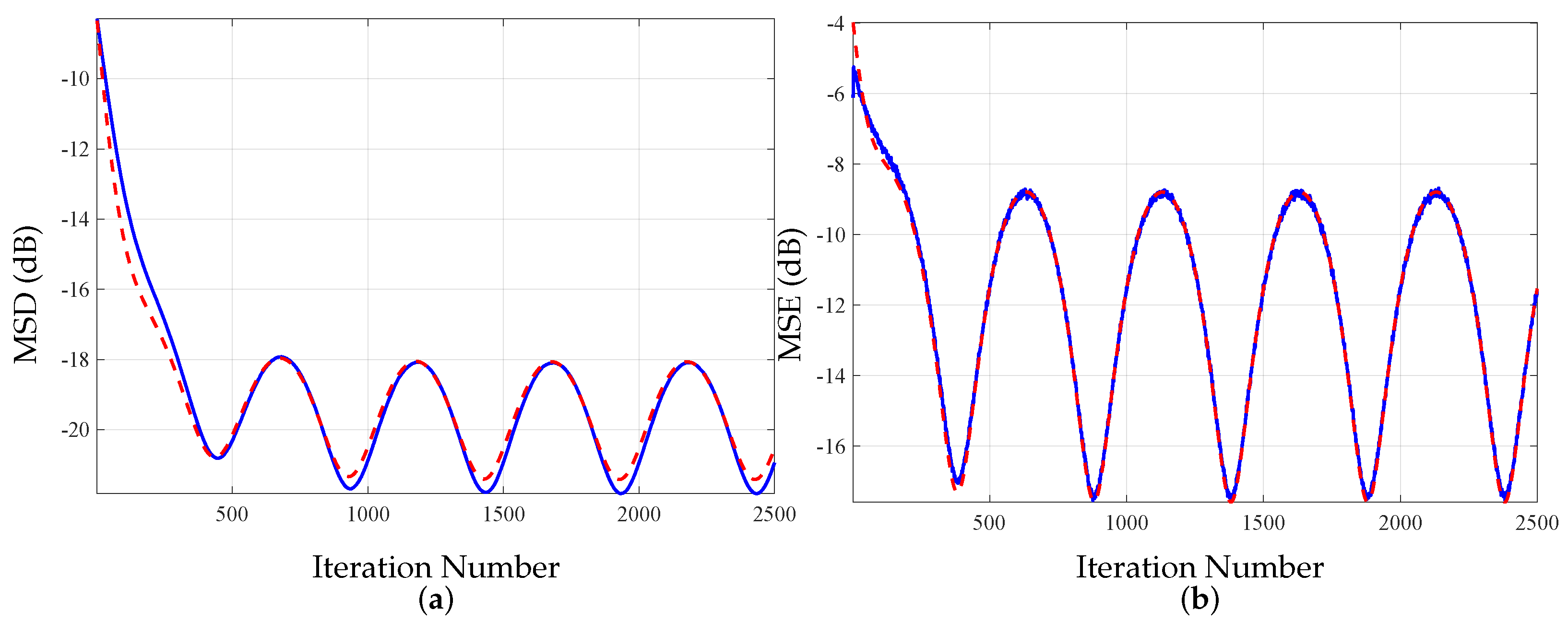
5.3. Tracking Analysis

The results presented in Figure 5 shows the ability of the proposed stochastic model to predict the tracking ability of the SPU-LMS-M-min algorithm. The plant to be emulated contains the first 32 coefficients from Model 2 of [28]. The additive noise, as well as the perturbation $\mathit{q}\left(k\right)$, are distributed according to a white Gaussian process.

Table 2. Parameters used in tracking simulations scenario.

Parameters	Figure 5
$\beta$	${10}^{-2}$
${\sigma }_{\nu }^2$	${10}^{-6}$
$H\left(z\right)$	$1-0.8z^{-1}+0.2z^{-2}$
${\sigma }_q^2$	${10}^{-15}$

presents the parameters used in the simulations.

The results shown in Figure 5 reveal the asymptotic MSD performance of the algorithm as a function of $\beta$. The excellent adherence between the experimental results and the theoretical forecast stands out. Note that there is a specific value of $\beta$ that optimizes the asymptotic performance, which is duly estimated by the elaborated theoretical analysis. This value of $\beta$ is high enough to allow the filter to follow the non-stationarity of the plant varying in time, but at the same time, it is not high enough to generate a lot of variability in the estimation process. Such high variability has repercussions on the second-order statistics (such as variance), which are captured by performance metrics.

In the following scenario related to Figure 6, the target is to identify ability of the proposed stochastic model in following the evolution of the MSD and MSE under a non-stationary ${{\sigma }_{\nu }}^2$. The plant to be identified contains the first 32 coefficients of Model 2 of [28]. The total number of blocks is $M=8$. To evaluate the accuracy of the behavior of the proposed model before a colored input signal, the input signal is generated by passing a Gaussian white noise of unitary variance through the filter $H\left(z\right)=1-0.8z^{-1}+0.6z^{-2}-0.1z^{-3}$. The parameters of SPU-LMS-M-min are: $\beta =8\times {10}^{-3}$ and the formula used for calculating ${\sigma }_{\nu }^2\left(k\right)$ is

$${\sigma }_{\nu }^2\left(k\right)={\overline{\sigma }}_{\nu }^2+Asin\left(2\pi f_{s}k\right),$$

(46)

where ${\overline{\sigma }}_{\nu }^2={10}^{-2}$, $A={10}^{-1}$ and $f_s=2\times {10}^{-3}$. Empirical results were obtained through $2\times {10}^4$ independent Monte Carlo trials. The results shown in Figure 6a reveal adequate correspondence between the theoretical and experimental MSD curves, both in steady-state and transient regimes. The results shown in Figure 6b, which take advantage of the same parameters as those of Figure 6a, reveal adequate correspondence between the theoretical and experimental MSE curves, both in steady-state and transient regimes.

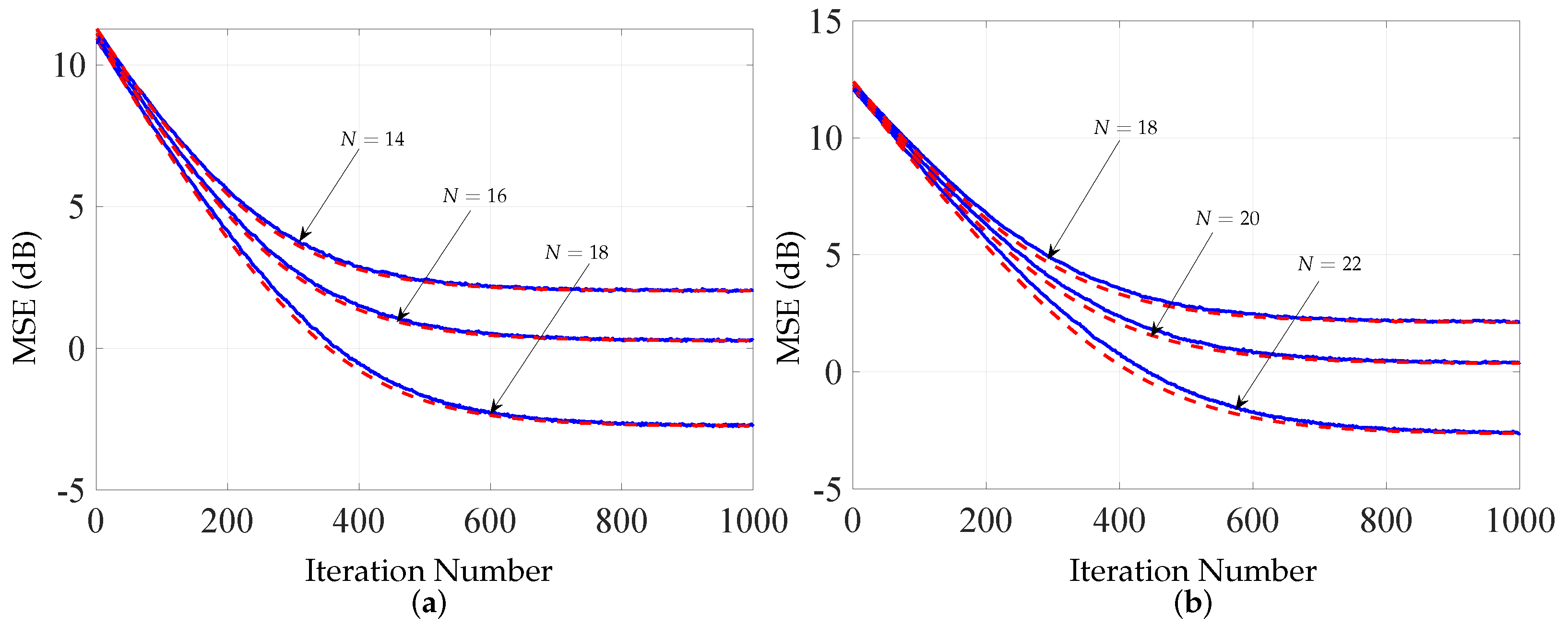
5.4. Deficient-Length Analysis

The results shown in Figure 7a,b reveal adequate correspondence between the theoretical and experimental MSE curves. Note that Equation (42) is very consistent with the dynamics of the MSE, both in transient regions, and especially in asymptotic regions. In these simulations, we used the following parameters: $\beta ={10}^{-2}$, ${\sigma }_{\nu }^2={10}^{-4}$, and $M=4$. The average results were computed from ${10}^5$ independent Monte Carlo trials. The ideal transfer function, $w_i^{★}$ was generated using the following interval:

$${\mathit{w}}_i^{★}=\left\{\begin{array}{cc}1,& \mathrm{for}i\in \{0,1,...,N-1\}\hfill \\ 0.5,& \mathrm{for}i\in \{N,N+1,...,N+D-1\}\hfill \end{array}\right.$$

(47)

Taking into account $N=C+D$, where $C\in \{12,16\}$ is the fixed number of filter coefficients, and $D\in \{2,4,6\}$ is the number of coefficients that exceed the filter amount. Note that Equation (42) is very consistent with the empirical dynamics of the MSE both in transient and asymptotic regions.

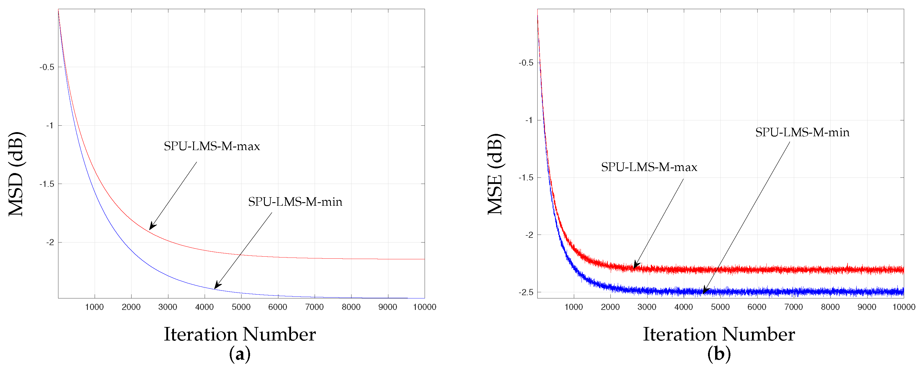
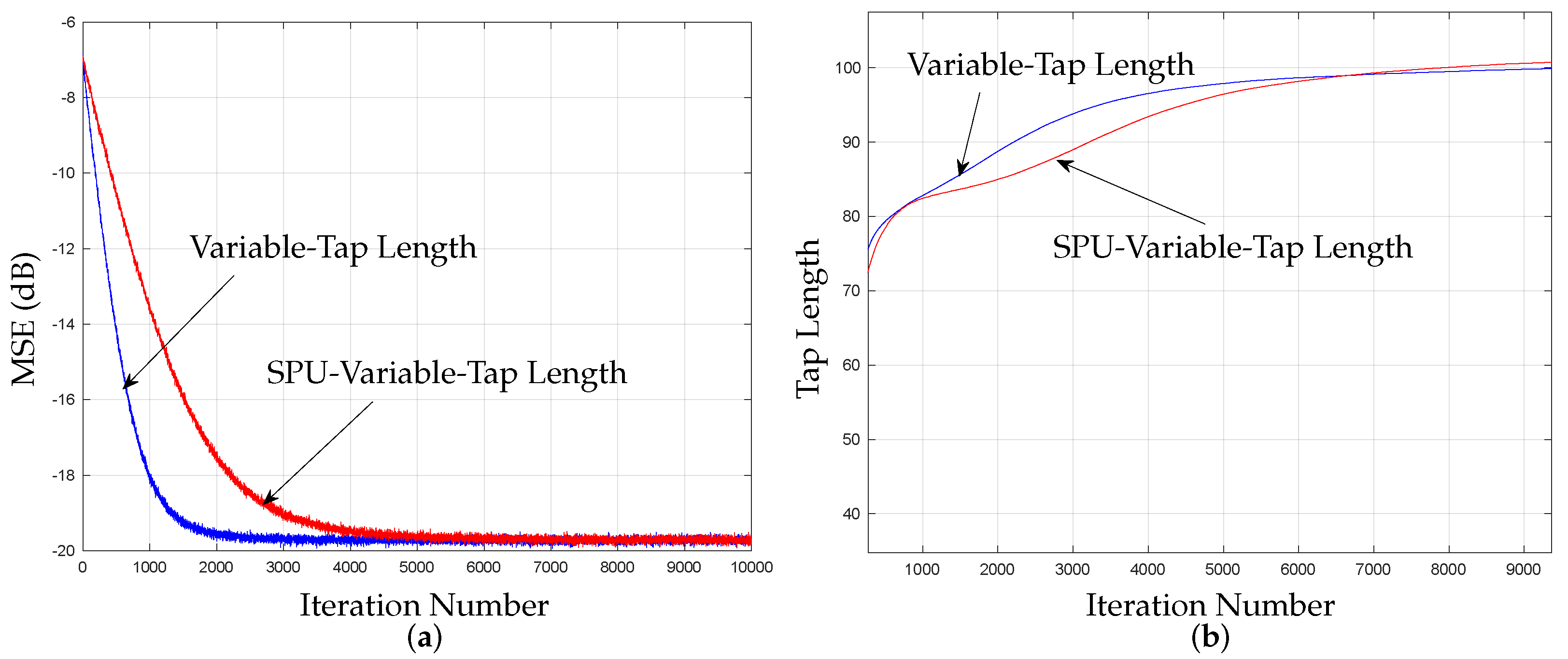
5.5. SPU-LMS-M-Min versus SPU-LMS-M-Max

Accordingly with classical approach for derivation of the SPU-LMS-M-max algorithm there was a statement never discussed before related to block selection, whose quadratic norm is the largest chosen [10] among all blocks, whereas in this paper the block with the smallest norm is elected. It should be observed that the advanced criterion selects a smallest norm (M-min) and shows better and more efficient results compared with the M-max variation, even-though under very intensive impulsive noise. Figure 8a shows comparisons between empirical MSD in which the first 64 coefficients of Model 3 of [28] are employed as the ideal transfer function. All empirical results were obtained by performing $2\times {10}^5$ independent Monte Carlo trials, and the additive noise derives from a white Gaussian process. The total number of blocks is $M=8$ and only $B=5$ blocks were updated. The input signal is generated by passing a unity-variance white Gaussian noise through the filter $H\left(z\right)=1-0.8z^{-1}+0.6z^{-2}-0.1z^{-3}$. The selected parameters are $\beta ={10}^{-3}$, ${\overline{\sigma }}_{\nu }^2={10}^{-8}$, and impulsive noise in a range from ${\overline{\sigma }}_{\nu }^2=2^{-1}$ to ${\overline{\sigma }}_{\nu }^2=1$ with 50% probability of occurrence. Figure 8b shows comparisons between empirical MSEs taking advantage of the same parameters as those employed in Figure 8a. In the settings depicted in Figure 8a,b, the reduction in the number of multiplications brought about by the proposed algorithm (compared to LMS) was approximately 20%. Note that a high-energy noise signal severely degrades the algorithm’s performance.

5.6. Extensions of the Proposed Framework Simulations

In accordance with the extension approach for SPU-LMS-M-max, incorporating a variable tap length algorithm, it is noteworthy that this method inherently utilizes a greater number of steady-state coefficients than strictly essential. Consequently, such an algorithm demands inefficient utilization of computational resources during steady-state operation. In response to this challenge, the amalgamation of SPU and VTL is proposed, thereby facilitating diminished computational costs while preserving an equivalent asymptotic performance. Despite the inevitable consequence of a controllable reduction in the convergence rate due to this integration, this trade-off can be effectively managed by judiciously selecting the fraction of coefficients to update. Thus, the proposed SPU methodogy was applied to an Acoustic Echo Cancellation (AEC) context, showcasing sustained asymptotic performance alongside diminished computational costs. This accomplishment is achieved at the cost of a controllable loss in the convergence rate, a parameter that remains adjustable by the designer. Figure 9a shows comparisons between empirical MSE for those algorithms VTL and SPU-VTL, where the 100 coefficients of Model 2 of [27] are employed as the ideal transfer function. All empirical results were obtained by performing $2\times {10}^4$ independent Monte Carlo trials, and the additive noise derives from a white Gaussian process. The total number of blocks is $M=8$ and only $85\%$ of the blocks were updated. The input signal is generated by passing a unity-variance white Gaussian noise through the filter $H\left(z\right)=0.35-z^{-1}+0.35z^{-2}$. The selected parameters were $\beta ={10}^{-2}$, ${\sigma }_{\nu }^2={10}^{-6}$, $\gamma =20$, $\alpha =4.{10}^{-4}$, $\delta =3$, and $\Delta =15$. While the transient regime underscores the superior convergence rate of Variable Tap Length (VTL), it is imperative to highlight that the utilization of Selective Partial Update with Variable Tap Length (SPU-VTL) concurrently diminishes computational complexity while maintaining an equivalent convergence rate during steady-state operation. Therefore, in the context of a Mean Squared Error (MSE) comparison, the judicious selection between VTL and SPU-VTL is pivotal for designers aiming to achieve specific targets. Figure 9b shows comparisons between empirical Tap Length over iterations used on VTL and SPU-VTL taking advantage of the same parameters as those employed in Figure 9a. In the configurations depicted in Figure 9a,b, the reduction in the number of multiplications resulting from the insertion of the SPU technique averaged 7.5%. Further, a detailed examination of Figure 9b reveals that in terms of energy efficiency, the application of tap length measurements by MSE calculation over up to ${10}^4$ iterations proved to be more effective during the transient regime. Moreover, in the steady-state regime, both algorithms demonstrated comparable performance.

Figure 10a,b present comparisons, measured in terms of Mean Squared Error (MSE), between traditional LMS and SPU algorithms applied to a practical scenario of Acoustic Echo Cancellation (AEC). In both instances, the parameters utilized included 20 coefficients representing the ideal transfer function, with SPU employing only 18 coefficients. The empirical results stem from $2.{10}^4$ independent Monte Carlo trials, incorporating white Gaussian noise as the additive element. The input signal is generated by passing unity-variance white Gaussian noise through the filter $H\left(z\right)=1-0.2z^{-1}+z^{-2}$. The coefficients of the ideal plant are described by, defined as $h_k=[cos{(0.2\times \pi \times (k+1\left)\right)]}^{-0.2\times (k+1)}$. The parameters applied are $\beta ={10}^{-2}$, ${\sigma }_{\nu }^2={10}^{-6}$ for Figure 10a and ${\sigma }_{\nu }^2={10}^{-2}$ for Figure 10b. In the settings depicted in Figure 10a,b, the computational cost reduction provided by the SPU-FX-LMS algorithm amounts to approximately 8%. Greater computational cost reductions can be achieved if the constraints of the application permit, given that such reductions entail a larger decrease in the convergence rate.

While both figures emphasize the superior convergence rate of FX-LMS during the transient regime, and in the steady-state regime where both FX-LMS and SPU-FX-LMS exhibit similarity, it is crucial to underscore that the implementation of SPU-FX-LMS concurrently reduces computational complexity while maintaining an equivalent performance during steady-state operation. Therefore, in the context of a Mean Squared Error (MSE) comparison, there is an important choice between FX-LMS and SPU-FX-LMS that becomes pivotal for designers with specific objectives in mind. Figure 10b illustrates similar comparisons of empirical MSE over iterations for FX-LMS and SPU-FX-LMS, leveraging the same parameters as in Figure 10a.

The theoretical framework expounded in the antecedent Figure 10a suggests a diminished computational demand. Nevertheless, a meticulous scrutiny of Figure 10b elucidates that, particularly in the presence of intensified noise, the augmentation of ${\sigma }_{\nu }^2$ values in the MSE calculations over a span of up to ${10}^4$ iterations proves to be notably efficacious when employing SPU-FX-LMS. This effectiveness arises from the algorithm’s capacity to optimize performance under conditions of high noise while concurrently exhibiting reduced computational complexity. The observed parity in steady-state results between SPU-FX-LMS and FX-LMS further underscores the former’s viability. Consequently, the strategic application of SPU-FX-LMS is advocated in scenarios characterized by constrained computational resources, even in the presence of substantial ambient noise. Notably, in applications such as Acoustic Echo Cancellation (AEC), the SPU strategy demonstrates potential benefits, including potential reductions in battery usage for hands-free devices, while maintaining robust echo cancellation capabilities in comparison to conventional LMS techniques.

6. Conclusions

This paper proposes a deterministic and local optimization problem, whose approximate solution puts forward a non-normalized adaptive algorithm with selective partial updates. Such an algorithm provides the designer with the ability to operate in a region of a trade-off between computational complexity and convergence rate. A stochastic model that predicts the learning capabilities of the new algorithm is derived and then extended to address first-order Markovian perturbations of the ideal plant in an identification scenario. Theoretical predictions are shown to be in close agreement with computer simulation results. The proposed methodology has been extended to configurations of automatic noise cancellation and time-varying filter length, providing the designer with the possibility to operate at various points where the convergence rate and computational complexity vary. Extensions to adaptive algorithms that exhibit higher computational cost (such as RLS [29]) and to the double-talk scenario constitute a promising line of future investigations.

References

1. Abadi, M.; Mehrdad, V.; Husoy, J. Combining Selective Partial Update and Selective Regressor Approaches for Affine Projection Adaptive Filtering. In Proceedings of the 2009 7th International Conference on Information, Communications and Signal Processing (ICICS), Macau, China, 8–10 December 2009; pp. 1–4. [Google Scholar]
2. Sayed, A.H. Adaptive Filters, 1st ed.; Wiley-IEEE Press: Newark, NJ, USA, 2008. [Google Scholar]
3. Wittenmark, B. Adaptive Filter Theory: Simon Haykin; Automatica, Elsevier Ltd: Amsterdam, The Netherlands, 1993; pp. 567–568. [Google Scholar]
4. Lara, P.; Igreja, F.; Tarrataca, L.D.T.J.; Barreto Haddad, D.; Petraglia, M.R. Exact Expectation Evaluation and Design of Variable Step-Size Adaptive Algorithms. IEEE Signal Process. Lett. 2019, 26, 74–78. [Google Scholar] [CrossRef]
5. Aboulnasr, T.; Mayyas, K. Complexity reduction of the NLMS algorithm via selective coefficient update. IEEE Trans. Signal Process. 1999, 47, 1421–1424. [Google Scholar] [CrossRef]
6. De Souza, J.V.G.; Henriques, F.D.R.; Siqueira, N.N.; Tarrataca, L.; Andrade, F.A.A.; Haddad, D.B. Stochastic Modeling of the Set-Membership- Sign-NLMS Algorithm. IEEE Access 2024, 12, 32739–32752. [Google Scholar] [CrossRef]
7. Wang, W.; Dogancay, K. Convergence Issues in Sequential Partial-Update LMS for Cyclostationary White Gaussian Input Signals. IEEE Signal Process. Lett. 2021, 28, 967–971. [Google Scholar] [CrossRef]
8. Wen, H.X.; Yang, S.Q.; Hong, Y.Q.; Luo, H. A Partial Update Adaptive Algorithm for Sparse System Identification. IEEE/ACM Trans. Audio Speech Lang. Process. 2020, 28, 240–255. [Google Scholar] [CrossRef]
9. Wang, W.; Doğançay, K. Partial-update strictly linear, semi-widely linear, and widely linear geometric-algebra adaptive filters. Signal Process. 2023, 210, 109059. [Google Scholar] [CrossRef]
10. Dogancay, K.; Tanrikulu, O. Adaptive filtering algorithms with selective partial updates. IEEE Trans. Circuits Syst. Analog. Digit. Signal Process. 2001, 48, 762–769. [Google Scholar] [CrossRef]
11. Akhtar, M.T.; Ahmed, S. A robust normalized variable tap-length normalized fractional LMS algorithm. In Proceedings of the 2016 IEEE 59th International Midwest Symposium on Circuits and Systems (MWSCAS), Abu Dhabi, United Arab Emirates, 16–19 October 2016; pp. 1–4. [Google Scholar] [CrossRef]
12. Gong, Y.; Cowan, C. An LMS style variable tap-length algorithm for structure adaptation. IEEE Trans. Signal Process. 2005, 53, 2400–2407. [Google Scholar] [CrossRef]
13. Li, N.; Zhang, Y.; Zhao, Y.; Hao, Y. An improved variable tap-length LMS algorithm. Signal Process. 2009, 89, 908–912. [Google Scholar] [CrossRef]
14. Zhang, Y.; Chambers, J. Convex Combination of Adaptive Filters for a Variable Tap-Length LMS Algorithm. IEEE Signal Process. Lett. 2006, 13, 628–631. [Google Scholar] [CrossRef]
15. Chang, D.C.; Chu, F.T. Feedforward Active Noise Control With a New Variable Tap-Length and Step-Size Filtered-X LMS Algorithm. IEEE/ACM Trans. Audio Speech Lang. Process. 2014, 22, 542–555. [Google Scholar] [CrossRef]
16. Kar, A.; Swamy, M. Tap-length optimization of adaptive filters used in stereophonic acoustic echo cancellation. Signal Process. 2017, 131, 422–433. [Google Scholar] [CrossRef]
17. Zhang, Y.; Li, N.; Chambers, J.; Sayed, A. Steady-State Performance Analysis of a Variable Tap-Length LMS Algorithm. IEEE Trans. Signal Process. 2008, 56, 839–845. [Google Scholar] [CrossRef]
18. Pitas, I. Fast algorithms for running ordering and max/min calculation. IEEE Trans. Circuits Syst. 1989, 36, 795–804. [Google Scholar] [CrossRef]
19. Boudiaf, M.; Benkherrat, M.; Boudiaf, M. Partial-update adaptive filters for event-related potentials denoising. In Proceedings of the IET 3rd International Conference on Intelligent Signal Processing (ISP 2017), London, UK, 4–5 December 2017; pp. 1–6. [Google Scholar]
20. Lara, P.; Tarrataca, L.D.; Haddad, D.B. Exact expectation analysis of the deficient-length LMS algorithm. Signal Process. 2019, 162, 54–64. [Google Scholar] [CrossRef]
21. Silva, M.T.M.; Nascimento, V.H. Convex Combination of Adaptive Filters with Different Tracking Capabilities. In Proceedings of the 2007 IEEE International Conference on Acoustics, Speech and Signal Processing-ICASSP ’07, Honolulu, HI, USA, 15–20 April 2007; Volume 3, pp. III–925–III–928. [Google Scholar]
22. Ibe, O.C. Basic Concepts in Probability. In Markov Processes for Stochastic Modeling; Elsevier: Amsterdam, The Netherlands, 2013; pp. 1–27. [Google Scholar]
23. Bershad, N.J.; Bermudez, J.C.M. Stochastic analysis of the LMS algorithm for non-stationary white Gaussian inputs. In Proceedings of the 2011 IEEE Statistical Signal Processing Workshop (SSP), Nice, France, 28–30 June 2011; pp. 57–60. [Google Scholar]
24. Mayyas, K. Performance analysis of the deficient length LMS adaptive algorithm. IEEE Trans. Signal Process. 2005, 53, 2727–2734. [Google Scholar] [CrossRef]
25. Le, D.C.; Viet, H.H. Filtered-x Set Membership Algorithm With Time-Varying Error Bound for Nonlinear Active Noise Control. IEEE Access 2022, 10, 90079–90091. [Google Scholar] [CrossRef]
26. Mossi, M.I.; Yemdji, C.; Evans, N.; Beaugeant, C. A Comparative Assessment of Noise and Non-Linear EchoEffects in Acoustic Echo Cancellation. In Proceedings of the IEEE 10th International Conference on Signal Processing Proceedings, Beijing, China, 24–28 October 2010; pp. 223–226. [Google Scholar]
27. ITU-T-2004. Digital Network Echo Cancellers (Recommendation); Technical Report G.168, ITU-T: Geneva, Switzerland, 2004. [Google Scholar]
28. ITU-T-2015. Digital Network Echo Cancellers (Recommendation); Technical Report G.168, ITU-T: Geneva, Switzerland, 2015. [Google Scholar]
29. Sadigh, A.N.; Zayyani, H.; Korki, M. A Robust Proportionate Graph Recursive Least Squares Algorithm for Adaptive Graph Signal Recovery. In IEEE Transactions on Circuits and Systems II: Express Briefs; IEEE: Piscataway, NJ, USA, 2024; p. 1. [Google Scholar] [CrossRef]
Figure 1. Block diagram of an adaptive filtering algorithm applied to systems identification.
Applsci 14 02775 g001
Figure 2. Block diagram of the FX-LMS algorithm.
Applsci 14 02775 g002
Figure 3. Theoretical (red dashed line) and empirical (blue solid line) evolution of the adaptive filter coefficients for B { 1 , 2 , 3 , 4 } . (a) Coefficient w 8 ( k ) ; (b) Coefficient w 34 ( k ) .
Applsci 14 02775 g003
Figure 4. Theoretical (red dashed line) and empirical (blue solid line) evolution of the adaptive filter coefficients for B { 1 , 2 , 3 , 4 } . (a) MSD (dB); (b) MSE (dB).
Applsci 14 02775 g004
Figure 5. Theoretical (red) and simulated (blue) steady-state MSD (in dB), as a function of β . The variance in the random perturbation is σ q 2 = 10 15 .
Applsci 14 02775 g005
Figure 6. Comparison of empirical results (a) MSD (dB); (b) MSE (dB). Theoretical result (red) and experimental result (blue), considering the colored input signal.
Applsci 14 02775 g006
Figure 7. Comparison between theoretical MSE (dashed red line) and empirical MSE (solid blue line) for the deficient-length scenario.
Applsci 14 02775 g007
Figure 8. Comparison between empirical SPU-LMS-M-max (red) and SPU-LMS-M-min (blue) for the very intense impulsive noise scenario. (a) MSD (dB); (b) MSE (dB).
Applsci 14 02775 g008
Figure 9. Comparison between empirical SPU-Variable Tap Length (red) and Variable Tap Length (blue). (a) MSE (dB); (b) Tap Length.
Applsci 14 02775 g009
Figure 10. Comparison between empirical SPU-FX-LMS (red) and FX-LMS (blue) for different intense noise scenarios. (a) σ ν 2 = 10 6 ; (b) σ ν 2 = 10 2 .
Applsci 14 02775 g010