Damage Classification of a Three-Story Aluminum Building Model by Convolutional Neural Networks and the Effect of Scarce Accelerometers

Abstract

Structural health monitoring (SHM) plays a crucial role in extending the service life of engineering structures. Effective monitoring not only provides insights into the health and functionality of a structure but also serves as an early warning system for potential damages and their propagation. Structural damages may arise from various factors, including natural phenomena and human activities. To address this, diverse applications have been developed to enable timely detection of such damages. Among these, vibration-based methods have received considerable attention in recent years. By leveraging advancements in computer processing capabilities, machine learning and deep learning algorithms have emerged as promising tools for enhancing the efficiency and accuracy of vibration-based SHM. This study focuses on the application of convolutional neural networks (CNNs) for the classification and detection of structural damage within a steel-aluminum building model. An experimental platform was devised and constructed to generate data representative of building damage scenarios induced by bolt loosening. Both the typical placement of sensors on each floor and the utilization of only one accelerometer were employed to understand the effect of scarcity of accelerometers. By subjecting the building model to controlled vibrations and environmental conditions, the response data from both sensor configurations were collected and analyzed to evaluate the effectiveness of the CNN approach in detecting structural damage under varying sensor deployment strategies. The findings demonstrate that the CNNs exhibited high accuracy in both damage classification and detection, even under scenarios with limited sensor coverage. Moreover, the proposed method proved effective in identifying structural damage within building structures.

1. Introduction

Engineering structures are subject to various types of damage throughout their lifespans, arising from environmental conditions, operational stresses, and human activities. Detecting and monitoring this damage is critical for ensuring structural integrity and safety. Traditional methods of inspection, such as visual assessment, are often labor-intensive and limited in their ability to provide comprehensive insights, particularly for large-scale structures. As a result, non-destructive techniques, including vibration-based structural health monitoring (SHM) systems, have gained prominence. Vibration-based SHM systems utilize sensors to monitor the dynamic response of structures to external forces or environmental conditions. These systems offer valuable insights into the structural health and performance of buildings, bridges, and other infrastructure. However, conventional approaches typically require sensors to be distributed across multiple locations within a structure, which can be impractical or costly to implement, especially for large or complex structures. To address this challenge, researchers have begun exploring alternative approaches to structural health monitoring that leverage advancements in artificial intelligence and machine learning. In particular, convolutional neural networks (CNNs) have emerged as a promising tool for analyzing sensor data and detecting structural damage. CNNs are well-suited for capturing complex spatial and temporal patterns in data, making them ideal for processing the multi-dimensional sensor data generated by SHM systems. This study focuses on investigating the efficacy of CNNs for structural damage detection in scenarios where sensor coverage is limited. By utilizing just one accelerometer placed on a structure, rather than multiple sensors distributed throughout, we aim to develop a cost-effective and practical solution for SHM. Through experimental testing on a three-story laboratory frame under different sensor configurations, we evaluate the performance of CNN-based damage detection algorithms. Additionally, we explore techniques such as data windowing to enhance the effectiveness of CNNs in scenarios with sparse sensor coverage.

2. Literature Review

Vibration-based building health monitoring systems, which have been developing recently, serve as an example of non-destructive testing systems. In vibration-based structural health monitoring or building damage detection, researchers focus on studies aimed at determining the location, time, and severity of damage in existing structures [1,2,3,4,5]. Many techniques have been developed to obtain information about structural health by examining the vibration responses of a structure [6,7,8,9,10]. In such techniques, the response of the building to forced or free vibrations by means of accelerometers placed at certain points of the building is tested to obtain information about the structural health by using different algorithms [10,11,12]. We can categorize vibration-based structural health monitoring methods into parametric and non-parametric approaches. In parametric vibration-based structural health monitoring, the dynamic parameters of the building (such as modal frequency, mass, rigidity, and mode shapes) are computed from the acceleration data collected by accelerometers [13,14,15,16,17,18]. In the parametric method, structural damage estimation is conducted by comparing the dynamic parameters of the damaged building with those of the undamaged building [19,20]. In non-parametric vibration-based structural health monitoring, on the other hand, an attempt to estimate structural damages is carried out by directly processing acceleration data. In certain studies, researchers have combined time series analysis with statistical classification to uncover building features that exhibit distinct responses in the event of damage from raw signals. Subsequently, these signals were monitored using a classification tool to assess the health status of the building [21,22]. With the advancement of machine learning algorithms, a subset of artificial intelligence, and the evolution of computer components capable of processing large datasets, machine learning has gained significant importance in various aspects of our lives. It has begun to streamline human activities across a wide spectrum, from gaming to military applications and from auto-completing search engine queries to enabling driverless vehicles. Artificial intelligence continues to perform tasks that either take humans a longer time to accomplish or are beyond human capability entirely. However, since the developers of artificial intelligence algorithms are currently human, it falls upon humans to identify the most suitable artificial intelligence model and hyperparameters for a given task. This process is time-consuming, particularly in the development of deep learning algorithms, and requires extensive research and expertise to make informed decisions [23].

Machine learning approaches can be categorized into three main types: supervised, unsupervised, and reinforcement learning. Supervised learning is a machine learning paradigm that involves mapping an input to an output based on sample input-output pairs [24]. In simpler terms, supervised learning can be described as teaching the algorithm using a dataset with labeled examples and then requesting the system to provide possible outputs for new inputs. On the other hand, unsupervised learning involves extracting patterns or structures from unlabeled data without any predefined categories or labels [25]. In other words, unsupervised learning entails classifying data based on their inherent similarities or differences without relying on predefined categories or labels for unclassified or unlabeled data. Finally, reinforcement learning is a machine learning approach inspired by behaviorism, focusing on determining the actions that subjects should take in order to maximize the rewards within a given environment [26]. In a recent study, researchers proposed a method for developing MISMs on structural systems, utilizing structured input data to enrich mechanical understanding. They explored graph neural networks (GNNs) as a means of representing and embedding knowledge about structural systems, particularly truss structures. Unlike traditional black box machine learning models, the proposed approach emphasizes the role of structural mechanics in defining the surrogate model, aiming to produce physically based outputs for the problem at hand. Specifically, the researchers developed MISMs to learn deformation maps of the system based on known structural features. Their approach was applied to both bidimensional and tridimensional truss structures, demonstrating superior performance compared with standard surrogate models [27].

In this study, supervised learning algorithms, particularly convolutional neural networks (CNNs), will be utilized. In data-driven machine learning methods, as the name suggests, having a sufficient amount of data is crucial for the algorithm to effectively learn the underlying system and produce accurate outputs. The process of finding or creating a dataset is often the most labor-intensive aspect of supervised machine learning.

Deep neural networks (DNNs) refer to cases where artificial neural networks (ANNs) contain more than three layers. Deep learning represents one of the latest advancements in machine learning, with widespread applications across various scientific fields. Deep learning continues to evolve and yield increasingly accurate results. In deep learning methods, particularly CNNs, the networks can autonomously learn to extract features directly from the raw data pertinent to the problem at hand, thereby maximizing classification accuracy. This inherent capability makes CNNs particularly appealing for complex engineering applications [28].

CNNs excel at capturing the spatial and temporal dependencies in signal data through the application of relevant filters. Traditionally, CNNs have been predominantly used in image recognition tasks within the literature. However, in recent studies, CNNs have also begun to be employed in vibration-based structural health monitoring systems, leveraging increased computational power. Yu et al. [29] developed a CNN to ascertain the location and extent of structural damage in a five-story building model. The authors aimed to detect damage in the building model by analyzing the acceleration data from the El Centro dataset. In a similar study, Dang et al. [30] employed a CNN to identify damage in a population of bridge structures constructed using a large number of random models. The damage characteristics of this population were extracted, and the CNN was subsequently utilized to detect damage in newly generated models. The results showed that employing acceleration signals as CNN inputs achieved the highest detection accuracy, reaching 99.4%. This underscores the efficacy of the proposed approach in enabling CNNs to identify damage across multiple structures.

This study aims to investigate the performance of a CNN in scenarios where there is an insufficient number of measurement sensors, meaning only one accelerometer is placed on the structure, neglecting the placement of one accelerometer on each floor as is typical. To achieve this, a three-story single-bay laboratory frame is experimentally examined under both sufficient and insufficient sensor configurations. In this context, the effectiveness of the CNN technique is enhanced by applying windowing to the transformed data. The results obtained indicate that the employed CNN approach can successfully estimate damage detection even in situations with limited sensor placement.

In order to validate the efficacy of a CNN in scenarios with limited sensor placement, the experimental test set-up serves as a critical component, providing real-world data for analysis and comparison. By meticulously configuring the three-story single-bay laboratory frame under both sufficient and insufficient sensor configurations, the experimental set-up simulates realistic conditions, allowing for a comprehensive evaluation of CNN performance. This set-up not only facilitates the investigation of a CNN’s capabilities in scenarios with limited sensor coverage but also enables the assessment of its robustness and reliability in practical structural health monitoring applications.

3. Experimental Test Set-Up

In the laboratory, a three-story aluminum building model was constructed and utilized as a test platform (Figure 1). The building model consisted of rectangular tube beam elements and flat bar column elements, with the connections between them provided by bolts. The bottom plate of the three-story building model was mounted horizontally and supported by two 400 cm long, 25 mm wide steel rails. A spring capable of working in the tensile direction was installed on the bottom surface of the table at the ground level of the three-story system and the plate supporting the entire system. The purpose of this spring was to prevent the system from moving away from the shaker. Additionally, an 8 mm diameter gear shaft connected to this spring and a knob were placed at the end to adjust the tension of the spring. This set-up reduced the collision effect between the shaker output shaft and the floor plate, which occurred at different vibration frequencies, and ensured proper shaking of the system. The floor table on the rails and the other parts of the system mounted on it could move horizontally and on a single axis. The floor table and columns were fixed with 4 M6 bolts made of A2 steel to prevent corrosion from moisture. The entire system was made of aluminum, except for the skid on which the floor table sat and the connection equipment. The total length of the system was 750 cm, the width was 350 cm, and the distance between the floors was 17 cm.

When any of the bolt connections were loosened, and the system was exposed to environmental and operational conditions, both nonlinear signals due to bolt loosening and signals due to noise were obtained from the sensors. These nonlinear signals represent damage. The primary objective of structural health monitoring is to distinguish the effects caused by damage from noisy signals due to environmental factors and use them as a damage index. By loosening the bolt and allowing 0.3 mm of axial movement from the nut’s contacted surface, a damage simulation was created. A feeler gauge was used to measure how far the nut moved. Since there were three bolts in total, a total of 2³ = 8 scenarios could be produced.

The building model was mounted on foam that could isolate the noise, sub-plates, rails, shafts, trolleys, shaker, and all mechanical connection equipment that made up the system. This foam reduces the transfer of external noise to the system [31].

Following the construction of the three-story aluminum building model and the establishment of the experimental set-up, the tests were conducted, employing both the three-accelerometer and single-accelerometer configurations. For the three-accelerometer set-up, the sensors were strategically placed on each floor of the building model to capture comprehensive vibration data across different levels. This configuration aimed to provide detailed insights into the structural response to various stimuli and potential damage occurrences. Conversely, in the single-accelerometer configuration, only one accelerometer was utilized, neglecting the typical placement of sensors on each floor. This scenario simulated situations with limited sensor coverage, which are common in practical applications where deploying multiple sensors might not be feasible due to cost or logistical constraints. By subjecting the building model to controlled vibrations and environmental conditions, the response data from both sensor configurations were collected and analyzed to evaluate the effectiveness of the CNN approach in detecting structural damage under varying sensor deployment strategies.

4. Materials and Methods

4.1. Dataset

At the end of the test period, a 3D tensor was obtained with dimensions of 8298 × 5 × 64. For each loosening case, the tests were repeated 8 times, resulting in a total of 64 datasets. The first column of the dataset concerns time (s), whereas the second, third, fourth, and fifth columns concern the accelerometer signals (m/s²). Notably, the ground acceleration data in the second column were not utilized in this analysis. To feed the data into the Conv1D layer, they needed to be reshaped into a one-dimensional format. Therefore, the data were reshaped so that the third axes were horizontally stacked on top of each other. This prepared the data to be fed into convolutional neural networks. Since the data were artificially created, the dataset was balanced (i.e., there were an equal number of examples for each damage case). Additionally, the states of the bolts in each damage case are presented in

Table 1. Damage cases with the states of the bolts.

Damage Case	Bolt 1	Bolt 2	Bolt 3
1	0	0	0
2	0	1	0
3	0	0	1
4	0	1	1
5	1	0	0
6	1	0	1
7	1	1	0
8	1	1	1

Here, “1” represents the system being damaged, while “0” shows that the system is healthy.

.

In neural networks, data are generally divided into training, validation, and test sets. It is noted that 8 tests were carried out for each of the 8 damage cases. The first 6 tests were chosen as the training set, while the seventh and eighth tests were designated as the validation and test sets, respectively.

4.2. Methods

CNN architectures come in various dimensions, including 1D, 2D, and 3D formats. Among these, 2D CNNs are most prevalent and are commonly employed for tasks such as image classification, similarity clustering, and object recognition in scenes. The rationale behind the prevalent use of 2D CNNs in image classification stems from the inherently two-dimensional nature of image data [32]. Conversely, Conv1D architectures are typically applied for analyzing time series data. Given that the vibration data obtained from building structures also exhibit temporal characteristics, Conv1D architectures can be effectively utilized for the classification of acceleration data [33].

In the context of this research, a convolutional neural network (CNN) model was developed. Although CNNs operate as black box systems, where input batches are processed to yield corresponding outputs, designing effective machine learning models involves selecting appropriate algorithms and techniques, which in turn require decisions regarding specific parameters [34]. In deep neural network models, designers must determine key factors such as dropout rates, the number of layers, and the quantity of neurons. However, deciding on these parameters is often not a straightforward process, as their optimal values may not be immediately apparent. These parameters, which vary depending on the problem and dataset, are known as hyperparameters. Different combinations of hyperparameters may yield varying levels of model performance, and selecting the most suitable combination is a crucial challenge. Typically, hyperparameter selection relies on the designer’s intuition, past experience, reflection on applications in related fields, current trends, and the inherent design characteristics of the model. However, recent advancements have introduced techniques aimed at systematically identifying the most appropriate hyperparameter combinations for optimal problem solving. The number of hyperparameters in a model can vary significantly, ranging from just a few to several hundred. Examples of hyperparameters include the number of layers and epochs, kernel size, stride, padding batch size, activation function, layer types, and units. Hyperparameter tuning is essential for creating the most effective model for a given dataset, and various methods exist for achieving this goal.

After discussing the basics of convolutional neural networks (CNNs) and their application in vibration-based structural damage detection, it is important to delve into the concept of hyperparameters and their significance in model design and performance optimization. In machine learning models, hyperparameters are parameters whose values are set before the learning process begins. These parameters govern the behavior of the model during training and influence its ability to learn from the data. Some common hyperparameters in CNNs include the following:

Number of Layers: This refers to the depth of the neural network, including convolutional layers, pooling layers, and fully connected layers. Deeper networks can potentially capture more complex patterns but may also be prone to overfitting.

Epochs: An epoch is one complete pass through the entire training dataset. The number of epochs determines how many times the model will see the entire dataset during training.

Kernel Size: In convolutional layers, the kernel size defines the spatial dimensions of the filter applied to the input data. Larger kernels capture broader patterns, while smaller kernels focus on finer details.

Stride: The stride parameter specifies the step size at which the kernel moves across the input data during convolution. A larger stride reduces the spatial dimensions of the output feature maps.

Padding: Padding is used to preserve the spatial dimensions of the input data when applying convolutional filters. It involves adding zeros around the input data to ensure that the output feature maps have the desired size.

Batch Size: The batch size determines the number of samples processed by the model in each training iteration. Larger batch sizes can accelerate training but may require more memory.

Activation Function: Activation functions introduce nonlinearity into the network and enable it to learn complex mappings between inputs and outputs. Common activation functions include ReLU, sigmoid, and tanh.

Dropout: Dropout is a regularization technique used to prevent overfitting by randomly deactivating a fraction of the neurons during training.

Learning Rate: The learning rate controls the step size of the gradient descent algorithm used to update the model weights during training. It influences the speed and stability of the training process.

Through meticulous tuning of these hyperparameters, researchers and practitioners can optimize the performance of CNNs for specific tasks and datasets, thereby enhancing generalization and predictive accuracy. Various techniques, such as grid search, random search, and Bayesian optimization, can be employed to identify the optimal combination of hyperparameters for a given problem.

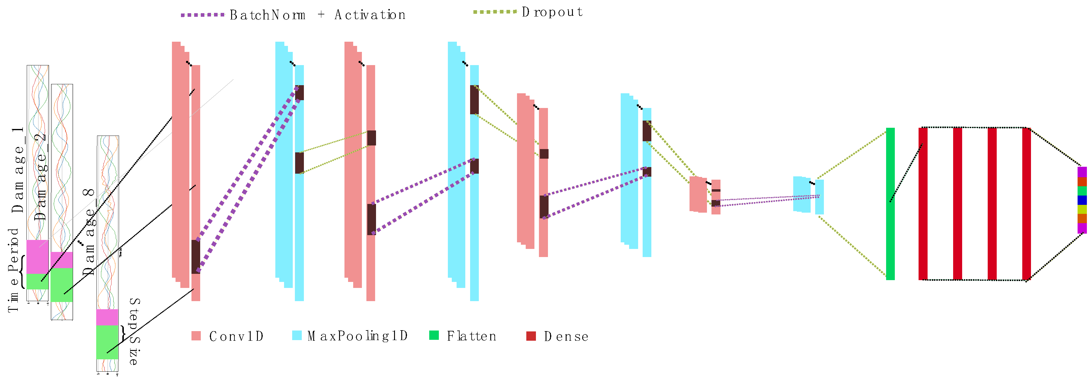
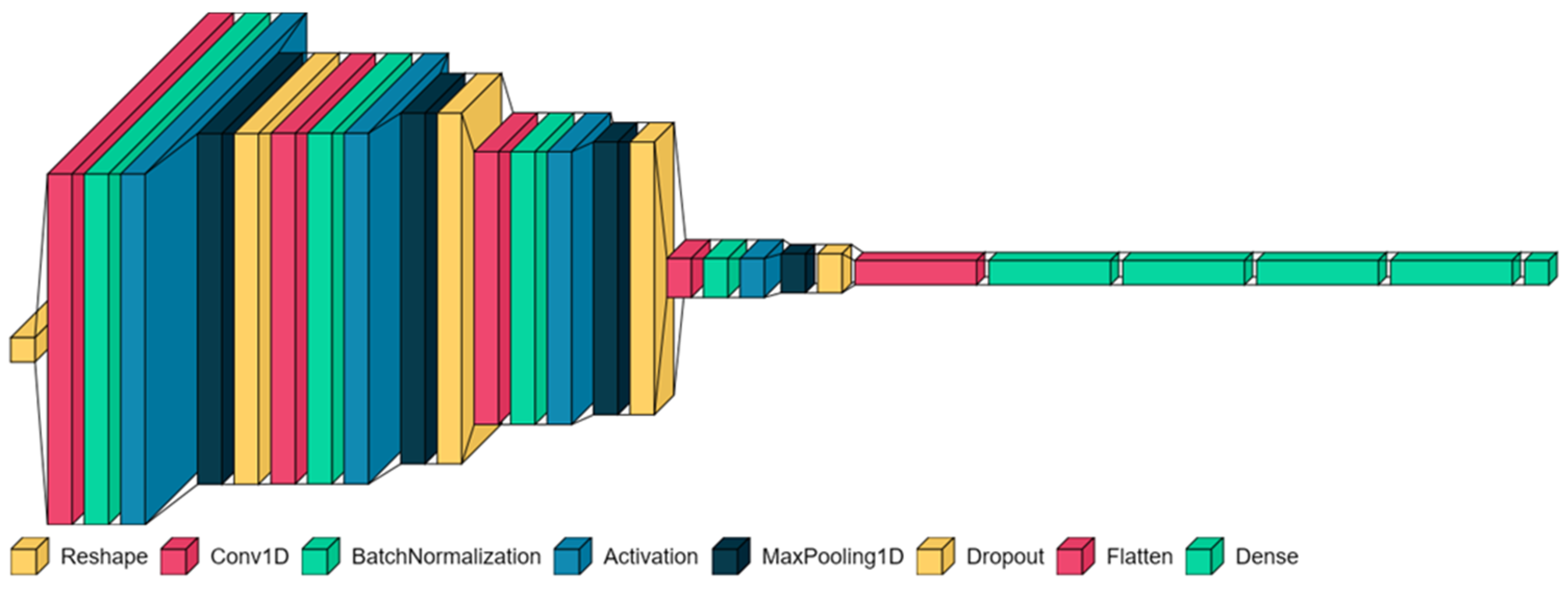
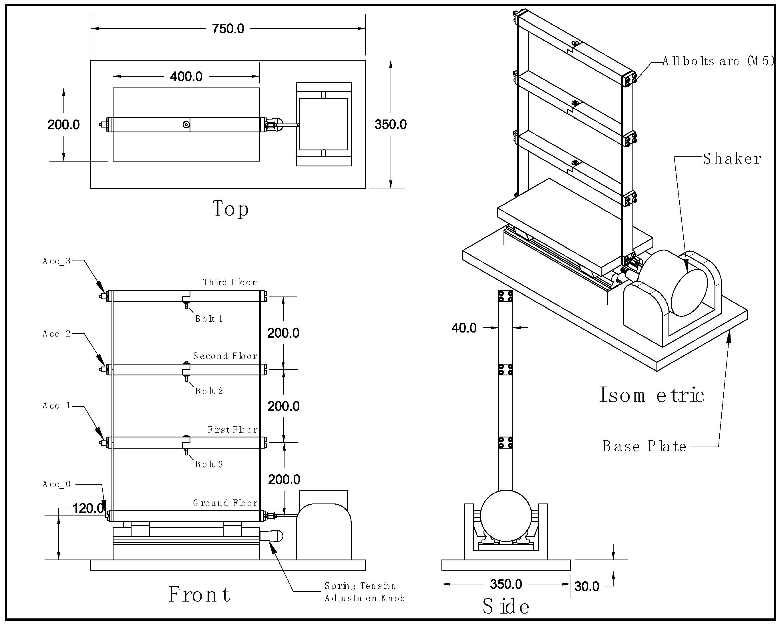
The overall CNN architecture for the current study is illustrated in Figure 2. Labeled acceleration data sampled at regular intervals were inputted into 1D convolutional layers. Interspersed between these layers were dropout layers, which served to mitigate overfitting of the neural network structure to the training data. Additionally, batch normalization layers were incorporated to normalize activations in the intermediate layers, thereby improving the accuracy.

In the upcoming section, we will detail a comprehensive strategy for hyperparameter optimization, a critical phase aimed at refining the effectiveness of our network architecture. Through extensive experimentation and systematic adjustment of the hyperparameters, our objective was to identify the optimal configuration that maximized the network’s performance across various metrics. This rigorous process ensured the robustness and adaptability of our model, allowing us to gain valuable insights into the complex interactions among different architectural components and their influence on the network’s predictive abilities.

Hyperparameter Tuning

The advent of deep learning introduced complex architectural structures with multiple layers, each governed by a set of hyperparameters determined by the designer. While some hyperparameters, such as optimization algorithms and activation functions, involve straightforward selection from a limited pool of options, others, including the number of layers and neurons, learning rates, and kernel sizes, require meticulous consideration due to their broad range of potential values. Choosing the appropriate hyperparameter values is often an iterative process, as the initial selections may not yield optimal results. Designers typically adjust these parameters iteratively, observing the model’s performance with each change to identify the most suitable hyperparameter combination. Additionally, automated methods exist to streamline this selection process. Two common hyperparameter tuning techniques are random search and grid search. In random search, values are randomly selected from predetermined ranges for each hyperparameter, with iterations continuing until the best-performing combination is found. On the other hand, grid search evaluates all possible combinations within specified ranges to identify the optimal hyperparameter group. The concept of random search for hyperparameter optimization was initially proposed by Bengio et al. [35]. Similar to grid search, this approach involves predetermining the hyperparameter ranges based on prior knowledge of the problem. 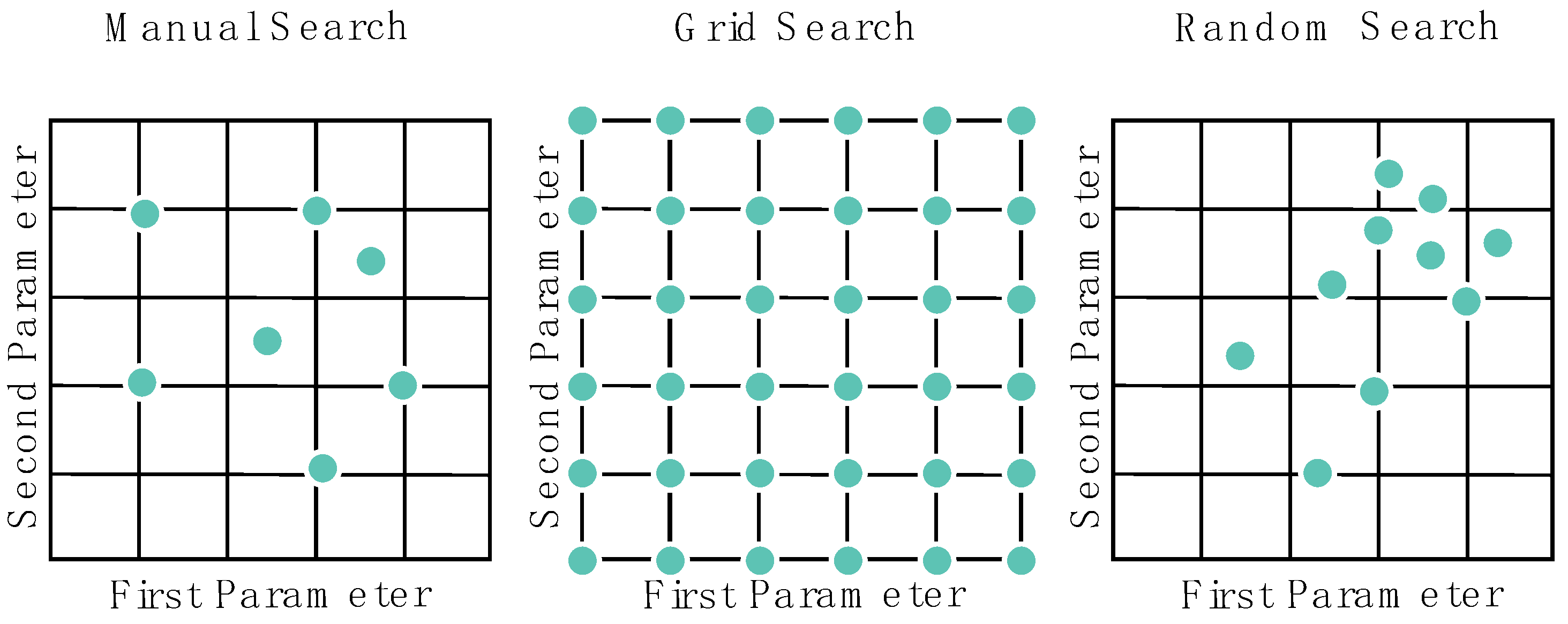However, instead of testing every value within these ranges, random values are selected and evaluated until the best-performing hyperparameter group is discovered or a desired performance level is achieved [36]. In addition to the techniques mentioned, Figure 3 illustrates a comparison of search algorithms, where the axes represent different hyperparameters. Each dot corresponds to a specific combination of hyperparameters evaluated by each method. In this visual representation, the different exploration strategies employed by each method can be observed, as well as how the hyperparameter space is navigated by them.

While random search and grid search are widely used methods, recent advancements like Hyperband have emerged to address the need for more efficient exploration of the hyperparameter space. Hyperband is a hyperparameter optimization technique that aims to efficiently search the hyperparameter space to find the optimal configuration for a machine learning model. It is designed to balance the trade-off between exploration and exploitation during the hyperparameter tuning process. The Hyperband algorithm works by iteratively allocating resources to a set of candidate hyperparameter configurations and then eliminating the poorly performing configurations based on their initial performance. It consists of two main components: random search and successive halving. Hyperband starts with a random sampling of hyperparameter configurations. Each configuration is evaluated using a predetermined amount of computational resources, such as the training time or epochs. This initial random search phase helps identify promising configurations to explore further. Then, Hyperband employs a successive halving strategy to efficiently allocate resources to the most promising configurations. This involves dividing the set of configurations into smaller subsets, or “brackets”, and allocating more resources to the configurations with the highest performance in each bracket. The configurations with worse performance are eliminated at each stage, allowing more resources to be focused on the most promising candidates. By iteratively applying random search and successive halving, Hyperband aims to quickly identify the best-performing hyperparameter configuration with minimal computational resources. It efficiently balances the exploration of the hyperparameter space with the exploitation of promising configurations, making it a popular choice for hyperparameter optimization tasks [37].

In the CNN model proposed in this study, after every Conv1D layer, there were max pooling layers and dropout layers. Max pooling layers help with reducing the spatial dimensions of the input data, thereby reducing the computational complexity of the model and extracting the most salient features from the data. This helps with capturing the essential information while discarding redundant or less important features, leading to better generalization and improved performance of the model. The dropout layers, on the other hand, were added to prevent overfitting of the CNN model to the training data. Overfitting occurs when the model learns to memorize the training data instead of generalizing patterns, leading to poor performance on unseen data. By randomly deactivating a fraction of the neurons during training, the dropout layers forced the model to learn more robust and generalized representations, thereby improving its ability to generalize to unseen data.

In the context of hyperparameter optimization, the “search space” refers to the range or set of possible values that each hyperparameter can take. Essentially, it encompasses all the potential options that the optimization algorithm explores when seeking the best-performing combination of hyperparameters. For example, if we consider hyperparameters like the learning rate, number of layers, and dropout rate, then the search space for each would consist of the various values or ranges within which these parameters could be adjusted. In essence, the search space defines the boundaries within which the optimization algorithm operates to find the optimal configuration for the neural network model. Maintaining a consistent search space across different experiments ensures fair comparisons between models trained on different datasets or with different configurations, allowing for a comprehensive evaluation of their performance. For example, if we were optimizing a CNN model using the HyperBand algorithm, then we would explore different configurations by varying the number of filters in the convolutional layers. This hyperparameter determines the number of filters or kernels that are applied to the input data during the convolution operation. Thus, for a specific experiment, we might try using 128 filters in one configuration, 160 filters in another, and so on up to 256 filters. Each configuration would be evaluated to determine its performance on the given dataset, and the algorithm would iteratively search through these options to find the best-performing combination of hyperparameters.

Table 2. Search space for the HyperBand algorithm.

Hyperparameter	Search Space
Number of filters	128, 160, 192, 224, 256
Conv1D layers	1, 2, 3, 4, 5, 6
Dropout	0.1, 0.2, 0.3, 0.4, 0.5
Dense layers	1, 2, 3, 4
Number of units in dense layer	128, 256, 512, 1024, 2048

displays the search space of the hyperparameters considered in the optimization process. Due to the extensive range of hyperparameters, the optimization algorithm necessitated a total of 9 hours to achieve optimal results. Generally, random search outpaces grid search in speed but often sacrifices performance. However, in this study, a novel approach to random search, termed the HyperBand hyperparameter optimization technique, was leveraged. This innovative method facilitated the attainment of a high level of accuracy in a relatively brief timeframe. Having max pooling layers and dropout layers after every Conv1D layer also meant that the number of Conv1D layers was the same as the number of max pooling layers and dropout layers. But the hyperparameters for the layers and the number of layers changed throughout the hyperparameter optimization procedure. After the best hyperparameters were found using the Hyperband, the model had been trained with the best hyperparamaters.

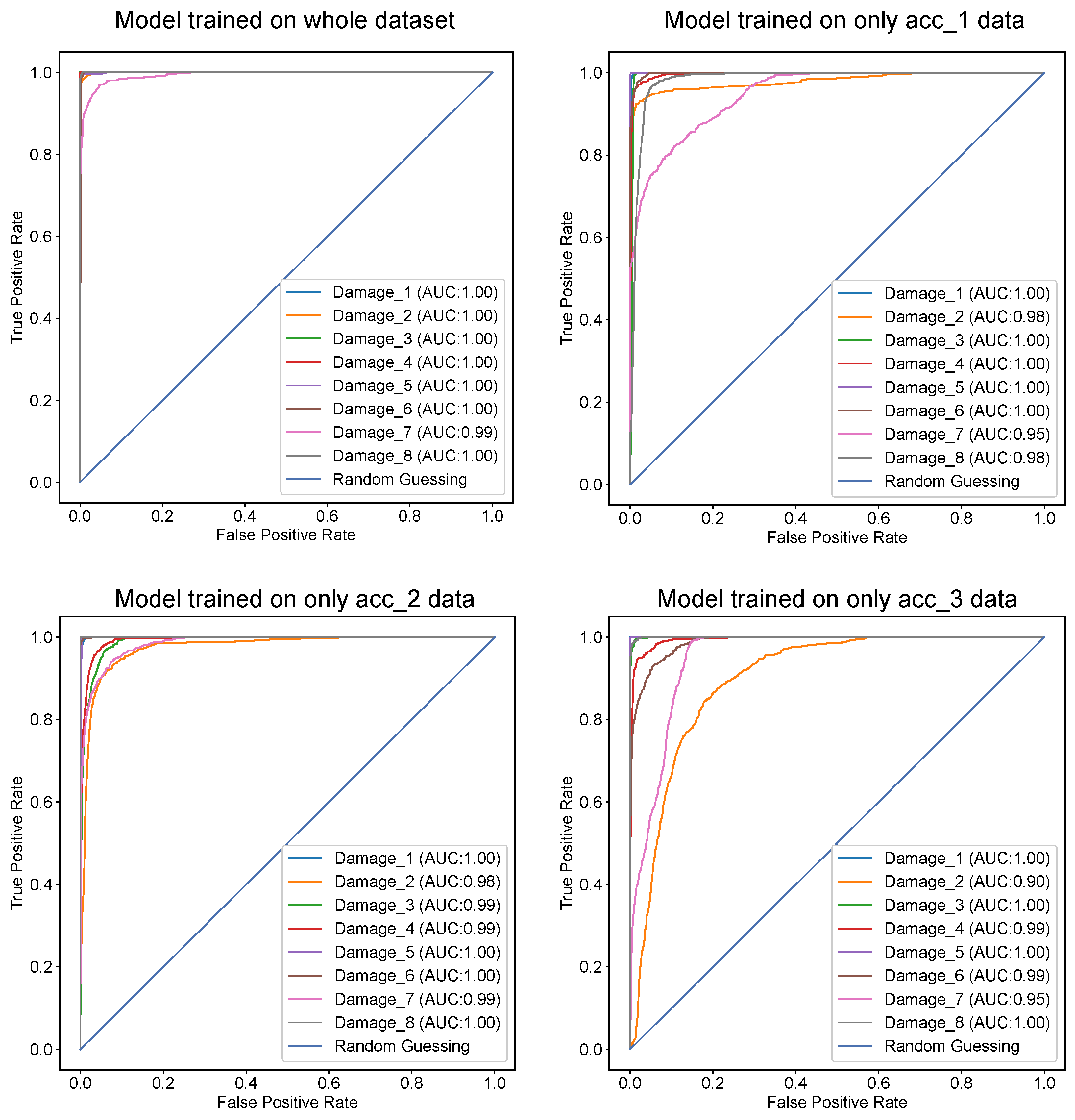
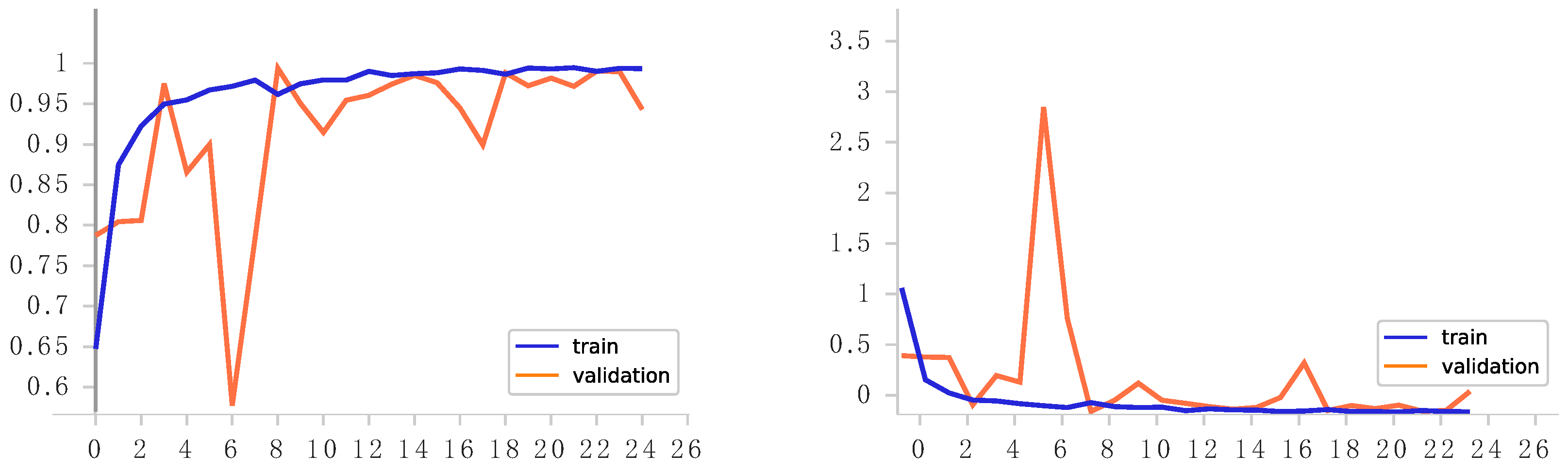
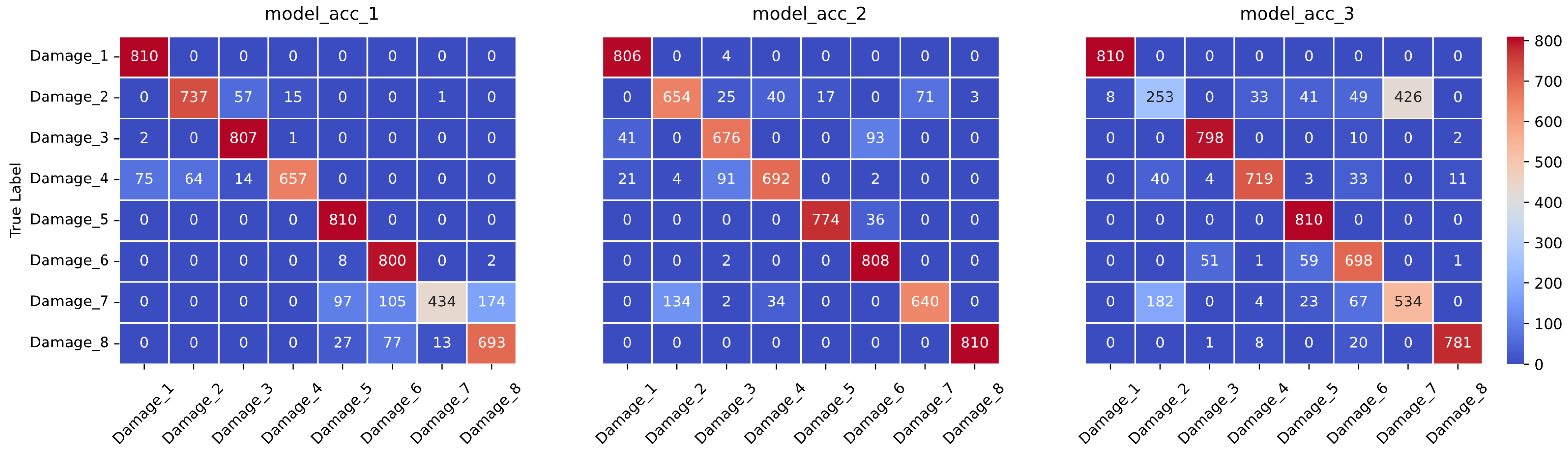
In this study, the presence of accelerometers on every story of the building facilitated comprehensive data collection for structural health monitoring. However, constraints such as scarcity of accelerometers or technical limitations may necessitate working with fewer sensors in some scenarios. Consequently, to address this variability in data availability, separate neural networks were trained using data from single accelerometers in addition to the complete dataset. This approach enabled a comparative analysis of the accuracy levels between the models trained on the entire dataset and those trained on subsets with fewer sensors. To ensure a fair comparison among these neural networks, the search space of the hyperparameters, optimization type, and other relevant parameters remained constant across all experiments. Detailed results, including the accuracy and loss values for each combination of hyperparameters and datasets, are provided in the Appendix A, Appendix B and Appendix C for thorough examination and comparison.

5. Results

The hyperparameter optimization results for the model trained on the whole dataset are provided in Appendix A. Despite even the worst-performing combination achieving an accuracy of over 90%, hyperparameter optimization was still necessary to discover the best combination of hyperparameters for improved performance on unseen test data. The best model exhibited a 98.9% training accuracy and 99% validation accuracy, outcomes achieved through hyperparameter optimization. The final model structure is given in Figure 4, and the hyperparameters are given in

Table 3. Optimum combination of hyperparameters obtained by random search method.

Hyperparameter	Optimal Value
n_layers	6
conv_0	288
conv_1	288
conv_2	224
conv_3	32
dropout	0.2
dense layers	3
n_nodes	256

.

The training and validation accuracies, as well as the loss versus epoch graphs, for the best-performing combination of hyperparameters are depicted in Figure 5. The optimized model achieved 98.3% accuracy and 0.02 loss on the training data and 94% accuracy and 0.018 loss on the validation data. These results indicate that the optimized model performed exceptionally well on the data on which it had been trained. However, the true performance would be assessed using the test data.

Before delving into the results, it is essential to understand some key evaluation metrics used to assess the performance of classification models: precision, recall, and F1 score, as well as the confusion matrix.

Precision, also known as the positive predictive value, measures the accuracy of positive predictions made by the model. It is calculated as the ratio of true positive predictions to the total number of positive predictions made by the model. A high precision score indicates that the model has fewer false positive predictions.

Recall, also known as the sensitivity or true positive rate, measures the ability of the model to correctly identify positive instances from the total actual positive instances in the dataset. It is calculated as the ratio of true positive predictions to the total number of actual positive instances. A high recall score indicates that the model can capture most of the positive instances.

The F1 score is the harmonic mean of the precision and recall. It provides a balance between precision and recall, especially in cases where there is an imbalance between the number of positive and negative instances in the dataset. The F1 score is calculated as shown in Equation (1):

$$2\times \frac{precision\times recall}{precision+recall}$$

(1)

In order to gauge the performance of the optimized model, it was subjected to evaluation using the test data. The confusion matrix, depicted in Figure 6, and the corresponding classification report in

Table 4. Classification report for test set.

Damage	Precision	Recall	f1-Score	Support
Damage_1	1.00	1.00	1.00	810
Damage_2	0.99	0.98	0.98	810
Damage_3	0.99	1.00	0.99	810
Damage_4	1.00	0.99	1.00	810
Damage_5	0.94	1.00	0.97	810
Damage_6	0.89	1.00	0.94	810
Damage_7	0.99	0.76	0.86	810
Damage_8	0.95	1.00	0.97	810
Accuracy			0.97	6480
Macro average	0.97	0.97	0.96	6480
Weighted average	0.97	0.97	0.96	648

provide insights into the model’s predictive capabilities. While the optimized model demonstrated high accuracy in predicting most damage cases, it exhibited some confusion, particularly with damage_7 classification. This poor performance for damage_7 might be attributed to various factors such as imbalanced data distribution, insufficient representation of damage_7 instances in the training dataset, or the presence of unique features in damage_7 cases that were not effectively captured by the model. Despite achieving F1 scores exceeding 90% for other damage categories, the F1 score for damage_7 stood at 86%, indicating relatively poorer performance in predicting instances of this specific damage type. However, it is worth noting that the overall accuracy for the test data remained commendable at 97%, surpassing acceptable levels.

Furthermore, considering the potential influence of overfitting in the single-accelerometer models, addressing this issue through future work is imperative. Further analysis and refinement are necessary to assess the generalization capability of these models and mitigate any adverse effects of overfitting.

It was stated there were a total of four accelerometers in every story and at the ground level. Hyperparameter optimization was also conducted for the neural network by using the data of the accelerometers on each floor separately, except for the ground acceleration data. The accuracy of the neural network on the test set was 89, 90, and 83% for acc1, acc2, and acc3, respectively. Even though the neural network was expected to perform worse with less data, the results for training of the neural network on single-accelerometer data were fairly satisfying. The confusion matrix and the classification report for all neural networks trained on the single-accelerometer data are presented in Figure 7 and

Table 5. Classification report for test set for each accelerometer configuration.

	Acc_1			Acc_2			Acc_3
Damage	Precision	Recall	F1 Score	Precision	Recall	F1 Score	Precision	Recall	F1 Score	Support
Damage_1	0.91	1.00	0.95	0.93	1.00	0.96	0.99	1.00	1.00	810
Damage_2	0.92	0.91	0.91	0.83	0.81	0.82	0.53	0.31	0.39	810
Damage_3	0.92	1.00	0.96	0.84	0.83	0.84	0.93	0.99	0.96	810
Damage_4	0.98	0.81	0.89	0.90	0.85	0.88	0.94	0.89	0.91	810
Damage_5	0.86	1.00	0.92	0.98	0.96	0.97	0.87	1.00	0.93	810
Damage_6	0.81	0.99	0.89	0.86	1.00	0.92	0.80	0.86	0.83	810
Damage_7	0.97	0.54	0.69	0.90	0.79	0.84	0.56	0.66	0.60	810
Damage_8	0.80	0.86	0.83	1.00	1.00	1.00	0.98	0.96	0.97	810
Accuracy			0.89			0.90			0.83	6480
Macro average	0.90	0.89	0.88	0.90	0.90	0.90	0.82	0.83	0.82	6480
Weighted average	0.90	0.89	0.88	0.90	0.90	0.90	0.82	0.83	0.82	6480

, respectively. Overall, the performance of the neural network dropped mildly. This was the expected result. However, given that the network was working with four times less data, the model was trained and tested far faster. This is an advantage because of the computing power. All data handling, training, and testing of the data were carried out on an AMD 3600X processor and RTX2070 GPU. While the hyperparameter optimization for single accelerometers took roughly 2 h for each, it took approximately 7 h for the whole dataset. This ratio is also valid for testing cases. All hyperparameter optimization results are given in the tables in Appendix B. A receiver operating characteristic (ROC) curve is a graphical plot that illustrates the performance of a binary classifier system as its discrimination threshold varies. It is created by plotting the true positive rate (TPR) against the false positive rate (FPR) at various threshold settings. The area under the curve (AUC) is a measure of the overall performance of the classifier, where a larger area under the curve represents better performance. ROC-AUC curves are a helpful tool for determining the accuracy of a binary classifier system. They can be used to compare different models, allowing for a better understanding of the performance of each model. Additionally, the AUC metric can be used to measure the overall performance of a model and help identify when a model is over- or underfitted. The ROC-AUC curves for all model are given in Appendix C.

6. Discussion

The achieved accuracy of 97% on the test set of the whole data reflects the effectiveness of the proposed CNN model in accurately classifying various types of structural damage. The performance of the CNN model in damage detection surpassed traditional methods, particularly visual inspection and non-destructive testing. The speed and accuracy of the proposed approach highlight the potential for transitioning from labor-intensive manual inspections to automated, data-driven methods.

The CNN’s ability to accurately classify and detect structural damage, even with noisy signals, underscores its efficacy in non-destructive testing. This is particularly valuable in scenarios where destructive testing is impractical or poses risks to structural integrity. The high accuracy of the model suggests its potential for real-time monitoring of structural health. Rapid and precise detection of damage types can facilitate timely interventions, preventing the progression of structural issues and enhancing overall safety.

An intriguing aspect of this study is the satisfactory performance achieved by the CNN models trained on individual accelerometer data from different floors. Despite the reduction in available data, the models demonstrated noteworthy accuracy levels: 89%, 90%, and 83% for acc1, acc2, and acc3, respectively. The ability to achieve meaningful results with models trained on data from a single accelerometer is promising for practical applications. This implies that in scenarios where sensor deployment is constrained or costly, a simplified monitoring set-up with fewer sensors may still provide valuable insights into structural health.

The reduced dataset for single accelerometers implies a more data-efficient training process. This efficiency is particularly beneficial in situations where data collection is challenging or expensive, showcasing the adaptability of the model to resource constraints. The training and testing of these single-accelerometer models were notably faster compared with the model trained on the entire dataset. This computational advantage is crucial for real-world applications, enabling quicker assessments and interventions in time-sensitive situations.

7. Conclusions

The findings of this study underscore the potential for practical and cost-effective structural health monitoring through the use of single accelerometers. The remarkable performance achieved by models trained on data from individual accelerometers introduces a paradigm shift in the deployment of monitoring systems. While the comprehensive model trained on the entire dataset remains a valuable tool, the demonstrated efficacy of simplified monitoring set-ups using fewer sensors holds significant promise.

The adaptability showcased in this research has far-reaching implications across various applications. In situations where resource constraints or retrofitting challenges pose limitations on deploying an extensive sensor network, the option of relying on strategically placed single accelerometers emerges as a viable and insightful alternative. This adaptability is particularly relevant in the context of existing structures, where the feasibility of retrofitting with modern sensor technology may be challenging.

The cost-effectiveness and efficiency of models trained on single accelerometer data pave the way for new avenues in structural health monitoring. The ability to obtain meaningful insights with a reduced number of sensors addresses practical challenges and opens doors for broader implementation. This adaptability could be instrumental in various fields, ranging from civil engineering and infrastructure monitoring to historical building preservation.

As we move forward, further research endeavors can delve into optimizing the integration of single accelerometers into structural health monitoring strategies. Exploring the optimal placement of these sensors and their combination with other non-intrusive sensing methods may enhance the overall accuracy and reliability of monitoring systems. This pursuit of efficiency aligns with the demand for accessible and practical solutions, particularly in scenarios where extensive sensor networks are not feasible.

In conclusion, this study not only contributes valuable insights to the field of structural health monitoring but also encourages a shift toward more accessible and efficient solutions. The adaptability demonstrated in this research underscores the potential for single accelerometers to play a pivotal role in shaping the future landscape of structural health monitoring, making it more feasible and impactful in real-world applications.

References

1. Altunışık, A.C.; Okur, F.Y.; Kahya, V. Modal parameter identification and vibration based damage detection of a multiple cracked cantilever beam. Eng. Fail. Anal. 2017, 79, 154–170. [Google Scholar] [CrossRef]
2. Xiang, J.; Liang, M.; He, Y. Experimental investigation of frequency-based multi-damage detection for beams using support vector regression. Eng. Fract. Mech. 2014, 131, 257–268. [Google Scholar] [CrossRef]
3. Wang, D.; Xiang, W.; Zhu, H. Damage identification in beam type structures based on statistical moment using a two step method. J. Sound Vib. 2014, 333, 745–760. [Google Scholar] [CrossRef]
4. Liu, J.; Lu, Z.; Yu, M. Damage identification of non-classically damped shear building by sensitivity analysis of complex modal parameter. J. Sound Vib. 2019, 438, 457–475. [Google Scholar] [CrossRef]
5. Yang, Y.; Zhu, Z.; Au, S.-K. Bayesian dynamic programming approach for tracking time-varying model properties in SHM. Mech. Syst. Signal Process. 2023, 185, 109735. [Google Scholar] [CrossRef]
6. Wickramasinghe, W.R.; Thambiratnam, D.P.; Chan, T.H.T.; Nguyen, T. Vibration characteristics and damage detection in a suspension bridge. J. Sound Vib. 2016, 375, 254–274. [Google Scholar] [CrossRef]
7. Labib, A.; Kennedy, D.; Featherston, C. Free vibration analysis of beams and frames with multiple cracks for damage detection. J. Sound Vib. 2014, 333, 4991–5003. [Google Scholar] [CrossRef]
8. Nandakumar, P.; Shankar, K. Structural crack damage detection using transfer matrix and state vector. Measurement 2015, 68, 310–327. [Google Scholar] [CrossRef]
9. Xu, Y.; Qian, Y.; Chen, J.; Song, G. Probability-based damage detection using model updating with efficient uncertainty propagation. Mech. Syst. Signal Process. 2015, 60–61, 958–970. [Google Scholar] [CrossRef]
10. Radzieński, M.; Krawczuk, M.; Palacz, M. Improvement of damage detection methods based on experimental modal parameters. Mech. Syst. Signal Process. 2011, 25, 2169–2190. [Google Scholar] [CrossRef]
11. Ding, Z.; Hou, R.; Xia, Y. Structural damage identification considering uncertainties based on a Jaya algorithm with a local pattern search strategy and L0.5 sparse regularization. Eng. Struct. 2022, 261, 114312. [Google Scholar] [CrossRef]
12. Patel, S.C.; Günay, S.; Marcou, S.; Gou, Y.; Kumar, U.; Allen, R.M. Toward Structural Health Monitoring with the MyShake Smartphone Network. Sensors 2023, 23, 8668. [Google Scholar] [CrossRef] [PubMed]
13. Sung, S.H.; Koo, K.Y.; Jung, H.J. Modal flexibility-based damage detection of cantilever beam-type structures using baseline modification. J. Sound Vib. 2014, 333, 4123–4138. [Google Scholar] [CrossRef]
14. Pooya, S.M.H.; Massumi, A. A novel damage detection method in beam-like structures based on the relation between modal kinetic energy and modal strain energy and using only damaged structure data. J. Sound Vib. 2022, 530, 116943. [Google Scholar] [CrossRef]
15. Yan, G.; Dyke, S.J.; Irfanoglu, A. Experimental validation of a damage detection approach on a full-scale highway sign support truss. Mech. Syst. Signal Process. 2012, 28, 195–211. [Google Scholar] [CrossRef]
16. Hosseinzadeh, A.Z.; Amiri, G.G.; Razzaghi, S.A.S.; Koo, K.Y.; Sung, S.H. Structural damage detection using sparse sensors installation by optimization procedure based on the modal flexibility matrix. J. Sound Vib. 2016, 381, 65–82. [Google Scholar] [CrossRef]
17. Gillich, G.-R.; Praisach, Z.-I. Modal identification and damage detection in beam-like structures using the power spectrum and time–frequency analysis. Signal Process. 2014, 96, 29–44. [Google Scholar] [CrossRef]
18. An, Y.; Spencer, B.F.; Ou, J. Real-time fast damage detection of shear structures with random base excitation. Measurement 2015, 74, 92–102. [Google Scholar] [CrossRef]
19. Devriendt, C.; De Sitter, G.; Guillaume, P. An operational modal analysis approach based on parametrically identified multivariable transmissibilities. Mech. Syst. Signal Process. 2010, 24, 1250–1259. [Google Scholar] [CrossRef]
20. Pintelon, R.; Guillaume, P.; Rolain, Y.; Schoukens, J.; Van Hamme, H. Parametric identification of transfer functions in the frequency domain-a survey. IEEE Trans. Autom. Control 1994, 39, 2245–2260. [Google Scholar] [CrossRef]
21. Kaloni, S.; Singh, G.; Tiwari, P. Nonparametric damage detection and localization model of framed civil structure based on local gravitation clustering analysis. J. Build. Eng. 2021, 44, 103339. [Google Scholar] [CrossRef]
22. Suwała, G.; Jankowski, Ł. Nonparametric identification of structural modifications in Laplace domain. Mech. Syst. Signal Process. 2017, 85, 867–878. [Google Scholar] [CrossRef]
23. Sarker, I.H. Machine Learning: Algorithms, Real-World Applications and Research Directions. SN Comput. Sci. 2021, 2, 160. [Google Scholar] [CrossRef] [PubMed]
24. Russell, S.J.; Norvig, P.; Davis, E. Artificial Intelligence: A Modern Approach, 3rd ed.; Prentice Hall: Upper Saddle River, NJ, USA, 2010; ISBN 978-0-13-604259-4. [Google Scholar]
25. Hinton, G.E.; Sejnowski, T.J. (Eds.) Unsupervised Learning: Foundations of Neural Computation; in Computational neuroscience; MIT Press: Cambridge, MA, USA, 1999; ISBN 978-0-262-58168-4. [Google Scholar]
26. Hu, J.; Niu, H.; Carrasco, J.; Lennox, B.; Arvin, F. Voronoi-Based Multi-Robot Autonomous Exploration in Unknown Environments via Deep Reinforcement Learning. IEEE Trans. Veh. Technol. 2020, 69, 14413–14423. [Google Scholar] [CrossRef]
27. Parisi, F.; Ruggieri, S.; Lovreglio, R.; Fanti, M.P.; Uva, G. On the use of mechanics-informed models to structural engineering systems: Application of graph neural networks for structural analysis. Structures 2024, 59, 105712. [Google Scholar] [CrossRef]
28. Shaheen, F.; Verma, B.; Asafuddoula, M. Impact of Automatic Feature Extraction in Deep Learning Architecture. In Proceedings of the 2016 International Conference on Digital Image Computing: Techniques and Applications (DICTA), Gold Coast, QLD, Australia, 30 November–2 December 2016; IEEE: Gold Coast, Australia, 2016; pp. 1–8. [Google Scholar] [CrossRef]
29. Yu, Y.; Wang, C.; Gu, X.; Li, J. A novel deep learning-based method for damage identification of smart building structures. Struct. Health Monit. 2019, 18, 143–163. [Google Scholar] [CrossRef]
30. Dang, V.-H.; Vu, T.-C.; Nguyen, B.-D.; Nguyen, Q.-H.; Nguyen, T.-D. Structural damage detection framework based on graph convolutional network directly using vibration data. Structures 2022, 38, 40–51. [Google Scholar] [CrossRef]
31. Pekedis, M. Detection of multiple bolt loosening via data based statistical pattern recognition techniques. J. Fac. Eng. Archit. Gazi Univ. 2021, 36, 1993–2010. [Google Scholar] [CrossRef]
32. Kang, L.; Kumar, J.; Ye, P.; Li, Y.; Doermann, D. Convolutional Neural Networks for Document Image Classification. In Proceedings of the 2014 22nd International Conference on Pattern Recognition, Stockholm, Sweden, 24–28 August 2014; IEEE: Stockholm, Sweden, 2014; pp. 3168–3172. [Google Scholar] [CrossRef]
33. Muralidharan, K.; Ramesh, A.; Rithvik, G.; Prem, S.; Reghunaath, A.A.; Gopinath, M.P. 1D Convolution approach to human activity recognition using sensor data and comparison with machine learning algorithms. Int. J. Cogn. Comput. Eng. 2021, 2, 130–143. [Google Scholar] [CrossRef]
34. Alzubaidi, L.; Zhang, J.; Humaidi, A.J.; Al-Dujaili, A.; Duan, Y.; Al-Shamma, O.; Santamaría, J.; Fadhel, M.A.; Al-Amidie, M.; Farhan, L. Review of deep learning: Concepts, CNN architectures, challenges, applications, future directions. J. Big Data 2021, 8, 53. [Google Scholar] [CrossRef] [PubMed]
35. Bergstra, J.; Bengio, Y. Random Search for Hyper-Parameter Optimization. J. Mach. Learn. Res. 2012, 13, 281–305. [Google Scholar]
36. Feurer, M.; Hutter, F. Hyperparameter Optimization. In Automated Machine Learning; Hutter, F., Kotthoff, L., Vanschoren, J., Eds.; The Springer Series on Challenges in Machine Learning; Springer International Publishing: Cham, Switzerland, 2019; pp. 3–33. [Google Scholar] [CrossRef]
37. Li, L.; Jamieson, K.; DeSalvo, G.; Rostamizadeh, A.; Talwalkar, A. Hyperband: A Novel Bandit-Based Approach to Hyperparameter Optimization. J. Mach. Learn. Res. 2016, 18, 1–52. [Google Scholar] [CrossRef]
Figure 1. Three views of the building model (adapted from [31]).
Applsci 14 02628 g001
Figure 2. Proposed neural network in present study.
Applsci 14 02628 g002
Figure 3. Comparison of search algorithms.
Applsci 14 02628 g003
Figure 4. A layered view of the optimized model.
Applsci 14 02628 g004
Figure 5. The training and validation accuracy (left) and training and validation loss (right) for the optimized model.
Applsci 14 02628 g005
Figure 6. Confusion matrix for the test set.
Applsci 14 02628 g006
Figure 7. Confusion matrix for all accelerometer configurations.
Applsci 14 02628 g007