1. Introduction
Selecting the relevant variables for modeling health outcomes and estimating the effects of said outcomes both frequently cause problems, with many inconsistencies regarding the best choice of the type of analysis, which becomes more acute with genetics due to the enormous volume of potential predictor variables. This problem is a driving force of our research.
A genetic variant is an alteration of a human DNA sequence that is shared by at least 1% of the population; this threshold emphasizes that the variant is not limited to a small number of people in which the alteration could have appeared via a de novo mutation, but is rather a genetic polymorphism among humans. Given that this variability is inherited and not caused by the environment, it is expected that genetic variants are responsible for all kinds of phenotypic variability within the species.
Many human diseases, although not exclusively caused by genetic factors, can be influenced by the genetic backgrounds of patients, e.g., some genes might exhibit DNA sequence variants that cause subliminal effects on their function, adding susceptibility to the individuals’ diseases; some DNA sequence variants might cause compensatory effects towards previous variants, thus leading to a lower probability of developing the condition; some DNA genetic variants might have better detoxification enzymes (again, due to genetic variants of those enzymes’ genes) and thus might even influence the effectiveness of the drugs given to the individuals in order to treat that same condition. All these differences will stratify the population according to disease susceptibility and prognosis and therapy outcomes, making DNA sequence variants particularly relevant for achieving more effective (personalized) medicine. Additionally, increasing our knowledge of the complex network of variants–genes–environment interactions relating to a particular disease is bound to improve our knowledge regarding the pathophysiology of the disease itself, with obvious gains in the advancement of biomedicine.
Alzheimer’s disease (AD) is a neurodegenerative condition that is initially characterized by memory impairment and cognitive decline, followed by behavior, speech, visuospatial orientation, and motor system alterations. It is a complex disorder, and its cause is multifactorial—both environmental and genetic factors can influence its onset [
1,
2]. One of the most challenging tasks of genetics research has been to uncover the genetic background of such diseases. Indeed, this is particularly challenging due to gene–gene and gene–environment interactions that can diminish and/or modulate the influence of individual genes or variants on the individual’s phenotype. Since most of these diseases would benefit from early diagnosis, meaning disease progression can be decelerated, it is important to be able to predict AD prior to the initial symptoms, making genetic risk calculation an appealing hypothesis. Nevertheless, the genetic variants that were associated with AD until present have a very low predictability power, due to the above-mentioned limitations, and it is therefore of great importance to obtain better statistics for this purpose.
Genome-wide association studies (GWAS) are populational studies in which individual DNA variants are tested for association with a particular trait. This is achieved by comparing, variant by variant, the allelic frequencies of the affected or unaffected subjects, specifically looking for discrepancies. Whenever an SNP exhibits a positive association with a trait, the alternative allele will be more frequent in people with that trait than in those without it. In recent years, GWAS have been conducted with genome-scale datasets of genetic variants (e.g., single nucleotide polymorphisms—SNPs). The statistics utilized within GWAS frequently use a model of regression; specifically, a logistic model for case/control designs or qualitative traits, and a linear model for quantitative ones. This allows for the inclusion of covariates, which can then accommodate for confounder effects or exclude any already known mediators of the studied trait. Most of these studies have relied on approaches consisting of the univariate analysis of the association of each SNP with the phenotype. Consequently, the possibility of a correlational and interactional structure between SNPs is not taken into account [
3]. This type of approach is not particularly well suited for the detection of small effects [
4], which can only become evident in the presence of other causal effects. In univariate approaches, multiple tests are performed independently, making it essential to correct the significance level in order to reduce the probability of type I errors (false positives). Frequently, however, the correction methods (e.g., Bonferroni) are too conservative, meaning it is not possible to detect any significant effects [
3], which can consequently lead to a paradoxical increase in type II errors (false negatives) [
5]. Another challenge in finding a plausible method to apply to genetic data is due to its high dimensionality; the number of variables (i.e., SNPs) is much higher than the number of individuals (
). Consequently, models are formed that can adjust data well, but that have poor predictive ability when applied to new data (overfitting and high variability). There are also correlational structures between the predictor variables, which can lead to multicollinearity problems [
6]. Furthermore, traditional multivariate regression models were not designed to deal with these problems. Therefore, to apply them to high dimensionality genetic data is not suitable.
One way to deal with the above-mentioned problems are penalization techniques, which have already been applied in the context of GWAS [
3,
7]. Penalization techniques refer to methods used to introduce a penalty or constraint on the model parameters during the training process. These techniques help to control the complexity of a model, reduce the risk of overfitting, and improve its generalization performance on unseen data. The penalized logistic regression combines traditional logistic regression with this penalty term in order to simultaneously perform classification and gene selection. This technique signifies the choice of a penalty parameter (λ), usually via cross-validation procedures, which define the extent of the predictor coefficient shrinkage. The Least Absolute Shrinkage and Selection Operator (LASSO) method was proposed by Tibshirani [
8], and is a penalization technique that imposes an L1—norm penalty. LASSO allows the explicit model simplification and, consequently, the interpretability improvement of the model once the insignificant predictor coefficients are forced to be equal to zero. For these reasons, the LASSO method has become very popular in high-dimensional data. However, this method does have limitations. For example, it cannot select more variables than the sample size. In the context of GWAS, there are high correlations between variables due to linkage disequilibrium or putative group structures. This leads to an instability in the selection of highly correlated variables via the LASSO method, since it arbitrarily only selects up to a few predictors, ignoring the others [
5,
9]. Ridge, proposed by Hoerl and Kennard [
10], is a penalization technique that uses an L2—norm penalty. In contrast with the LASSO method, Ridge does not have sparse properties in terms of the coefficients estimates as none of them are equal to zero [
11]. However, Ridge deals with higher correlations between predictors much better since it shrinks the coefficients of the correlated predictors. To achieve a technique with better performance, Zou and Hastie proposed a novel tool that consists of a linear combination of an L1—norm penalty and an L2—norm penalty, which is known as Elastic-Net [
12]. In Elastic-Net regression, the balance between the L1 and L2 regularization penalties is controlled by the α parameter, which has a scalar value ranging from 0 to 1. Elastic-Net can achieve sparse coefficient estimates and can work appropriately with the correlations between predictors [
11]. While LASSO regression (α = 1) excels in variable selection by forcing some coefficients to be equal to zero, Elastic-Net regression (0 < α < 1) provides a compromise between LASSO and Ridge regression, allowing for variable selection, while also handling multicollinearity more effectively.
As mentioned above, penalized regression models provide the choice of a penalty parameter (λ), usually through via cross-validation procedures, which establishes the estimation of predictors coefficients and, consequently, the selection of the most important predictor variables. The penalization parameter is sensitive to the data, and, in each iteration of cross-validation, a different parameter value can be chosen. As a result, in each iteration of cross-validation, the variable selection is not the same. In general, several runs of the same procedure led to different results, which means that the procedure is not stable. Additionally, the choice of the analysis method can affect the number and type of the selected features, the coefficient estimates, and the accuracy and precision of the coefficient estimates, and the performance depends on the characteristics of the data [
13].
Developing procedures that have been adapted to a large volume of data, which have stability in the identification of influential predictor variables and in the estimation of their explanatory effects, is imperative.
Therefore, the main goal of this work is to provide a new shrinkage regression procedure with stable variable selection for structures with a much higher number of variables than individuals. This procedure will then be applied as a proof of concept to the Alzheimer’s Disease Neuroimaging Initiative (ADNI) public dataset in order to identify the SNPs that are associated with AD, thus circumventing the above-mentioned limitations.
2. Materials and Methods
ADNI genotype data. The data used in this study were obtained from the ADNI public dataset; more specifically, from the ADNI-1 study (
https://adni.loni.usc.edu/about/adni1/, accessed on 1 February 2023). The individuals in this dataset underwent genotyping via the Illumina Human610-Quad BeadChip. The dataset contains the genotypic information of 599,011 SNPs from 757 individuals; 344 individuals had been diagnosed with Alzheimer’s disease (IAD), 210 individuals were perceived as cognitively normal (ICN), and 203 individuals had mild cognitive impairment (IMCI).
The data were submitted to quality control and population stratification, which were carried out in accordance with the procedure described by Anderson and others (2010) [
14], and was conducted using the PLINK software [
15] (version 1.9). To perform our study, we considered genotypic data from IAD and ICN individuals with western European ancestry, and information regarding probes that were dedicated to copy number variation was excluded. During the quality control procedure, a total of 103 samples were excluded. The exclusions were made as follows: 2 samples due to gender discrepancies; 96 samples due to divergent ancestry; 16 samples with a heterozygosity rate higher than expected; 2 samples due to non-reported relatedness to another participant of the study; and 4 samples with more than 5% missing genotypes. Additionally, for the initial 599,011 genotyped SNPs, we used filters to allow for the exclusion of SNPs with a missing rate higher than 5% (19,406), deviation from the Hardy–Weinberg equilibrium (130), and for having a minor allele frequency lower than 5% (61,218). The criteria used in data filtering and variable selection aligned with the guidelines for GWAS [
16]. Also, the missing rate of genotyped SNPs was compared between cases (IAD) and controls (ICN), and no significant differences were detected [
14]. An imputation was made to fill in missing genotypes using the
bigsnpr R package, namely the
snp_fastImpute method with the default parameters. Therefore, the final database was composed of 451 individuals, with 163 ICN (36.1%), 288 IAD (63.9%), and 518,257 SNPs.
Dataset handling. The data were divided into the two following datasets: a training set and a test set. The training set included 70% of the initial sample (116 ICN—36.7%; 200 IAD—63.3%), and was used to perform variable selection, as well as to build the prediction models. The test set included the remaining 30% (47 ICN—34.8%; 88 IAD—65.2%), and was used to assess the performance of the prediction models. This division was made randomly, and was stratified by the attributes of the dependent variable (IAD and ICN) in order to maintain the correct proportion of cases and controls.
Stable variable selection method with shrinkage regression. The proposed method analyzes and combines the results of the repeated applications of a penalized regression model on the training dataset.
The main objective of our procedure is to identify the most important variables and to define the corresponding regression coefficient using a measure of the relative quality of fit of each model. Variables that are selected more often in higher quality models will have greater potential to be selected for the final model. In fact, the “variable weight” (defined below) depends not only on the frequency of the selection of the variable in all models, but also on the inherent quality of the fit of each model. Therefore, the proposed variable selection procedure is more restrictive than the usual correspondent penalized regression approach.
The final regression coefficient of the relevant variables is calculated based on the coefficients obtained in each repetition of the penalized regression model. Following the same reasoning as the selection of the relevant variables, the coefficients associated with better quality models will greatly contribute to the overall value of the coefficient of the predictor variable. This final coefficient indicates whether the variable contributes positively or negatively to the outcome of the study. In the practical application being analyzed, this coefficient allows us to conclude whether the variable is a risk factor or a protection factor for Alzheimer’s disease.
In short, from several sets of selected variables, a single set of (the most relevant) variables is obtained, with a regression coefficient being assigned to each one.
To enhance the clarity of the process, the description of the proposed procedure was divided into three steps. First, several runs of the same penalized regression method are performed, and the result of each model is associated with a relative goodness-of-fit weight (step 1). Then, a global weight is assigned to each variable, defined as the sum of the weights of all the penalized models in which the variable was selected, representing its relative importance across the penalized models. If a variable’s weight exceeds a defined threshold, it is then selected for the final model (step 2). The coefficient estimate for each selected variable is determined as the average of its estimated coefficients in each penalized model, weighted by the relative goodness-of-fit weight of the model (step 3). The procedure is detailed below, and the graphical summary of the algorithm is available in the
Supplementary Materials.
Penalized regression models (Step 1). Repeated applications of a penalized regression model are conducted on the training dataset. Each repetition of the penalized regression model generates a set of predictor variables, which may not be the same. The Akaike’s information criterion (AIC) was calculated for each model, and the difference between the AIC and the AIC of the best model was calculated (a higher AIC means a lower fitness):
The smaller this difference, the better the model’s fit for the data. These differences allowed us to obtain the Akaike’s weight for each model using the following equation:
Now, the higher the value of this measure, the better the model’s quality of fit. The model Akaike’s weight is used in the next steps to define the variables across all penalized models and the regression coefficient in the final model.
Stable variable selection (Step 2). At this point, for each α-penalized regression technique, we obtained R models, and each one was assigned an Akaike’s weight. The next challenge was how to combine these weights for the estimation of the relative importance of each predictor. We defined the variable weight as the sum of the Akaike’s weight of all repeated penalized models in which the variable appears.
where
is an indicator vector of the non-null
th coefficient, and
is the number of variables. The criterion for classifying a variable as important was its weight,
, being at least 0.8. This importance threshold, in general, demonstrated good properties, allowing the minimization of the occurrence of type I and II errors [
17].
Model coefficients estimation (Step 3). In the final model, only the important predictors were considered; that is, the predictors with a weight of at least 0.8. For these, the estimated coefficient was defined by an overall weighted coefficient as follows:
where
is the coefficient estimate of the predictor in the model obtained in run
, and
is the Akaike’s weight of that model. For each of the estimated parameters,
, a weighted variance was also calculated as follows:
Therefore, it was possible to calculate an asymptotic Z confidence interval for each estimated parameter. The significance level used was 5%.
Models’ performance metrics and comparison. We analyzed the training dataset, which consisted of 316 individuals (116 ICN; 200 IAD) and 518,257 SNPs. The proposed procedure was applied for the two following scenarios: one considering only the SNPs (from here on referred to as “Scenario SNPs”), and another considering SNPs that was adjusted to also consider the covariates of age, sex, educational level, and APOE4 genotype (here on referred to as “Scenario SNPs + Cov”). Therefore, for each value of the α parameter, two final models were proposed. The performance of the models was evaluated on the test dataset, focusing on the area under the curve (AUC), the accuracy, and the F1-measure.
Traditional logistic regression (without shrinkage) is one of the most used methods with which to model binary outcomes; however, it can only be used when the number of variables is lower than the number of observations. To overcome this issue, a penalized regression technique can be applied before traditional logistic regression. We compared each final model with the corresponding traditional logistic regression model, built based on the same set of selected variables, in order to discuss the impact of shrinkage on the estimation of the coefficients (effect sizes). We also compared the two models using the above-mentioned performance metrics.
Technical details. The
![Applsci 14 02572 i001]()
language was used to carry out the statistical analysis.
In this work, prediction models were constructed using two penalized regression techniques, namely LASSO (α = 1) and Elastic-Net (0 < α < 1), for the α values in the grid {0.75, 0.50, 0.25, 0.10, 0.05, 0.01}. For each value of α, we obtained models. For each model, the value of the penalization parameter was achieved via a 10-fold cross-validation, and the model with the lowest validation error (deviance) was chosen. The generalized linear models, made via the penalized maximum likelihood, were obtained using the cv.glmnet R function, available in the glmnet package, using the default parameters.
3. Results
As expected, multiple runs of the same α-penalized regression procedure led to different results, confirming the instability of such procedures in contexts where the number of variables (i.e., SNPs) is much higher than the number of individuals. Indeed, there was a large variability in the number of selected variables across the 100 penalized regression models, both in cases where models were fitted to covariates (Scenario SNPs + Cov) and in which they were not (Scenario SNPs).
As shown in
Table 1, for all values of α, there was a large dispersion in the number of selected variables. For example, in Scenario SNPs and α = 0.01, the number of selected variables ranged from 0 to 6886. In both scenarios, the range and the maximum number of selected variables generally increased as the α value decreased. In relation to the median number of selected variables, a tendency to increase as the value of α decreased was also observed in Scenario SNPs + Cov. Although this trend was not observed in the SNP scenario for alpha values ranging between 0.05 and 1, the median number of the selected variables increased substantially for the model where α = 0.01 (
Figure 1).
Regarding the final models, which were built based on the proposed procedure, the largest number of selected variables occurred when α = 1 (with 11 variables) in Scenario SNPs, and when α = 0.01 and α = 0.05 (with 9 variables) in Scenario SNPs + Cov. In the latter scenario, the
APOE4 genotype covariate was always selected. It should be noted that, in the SNP scenario, there were several alpha values for which no variables were selected (
Table 2).
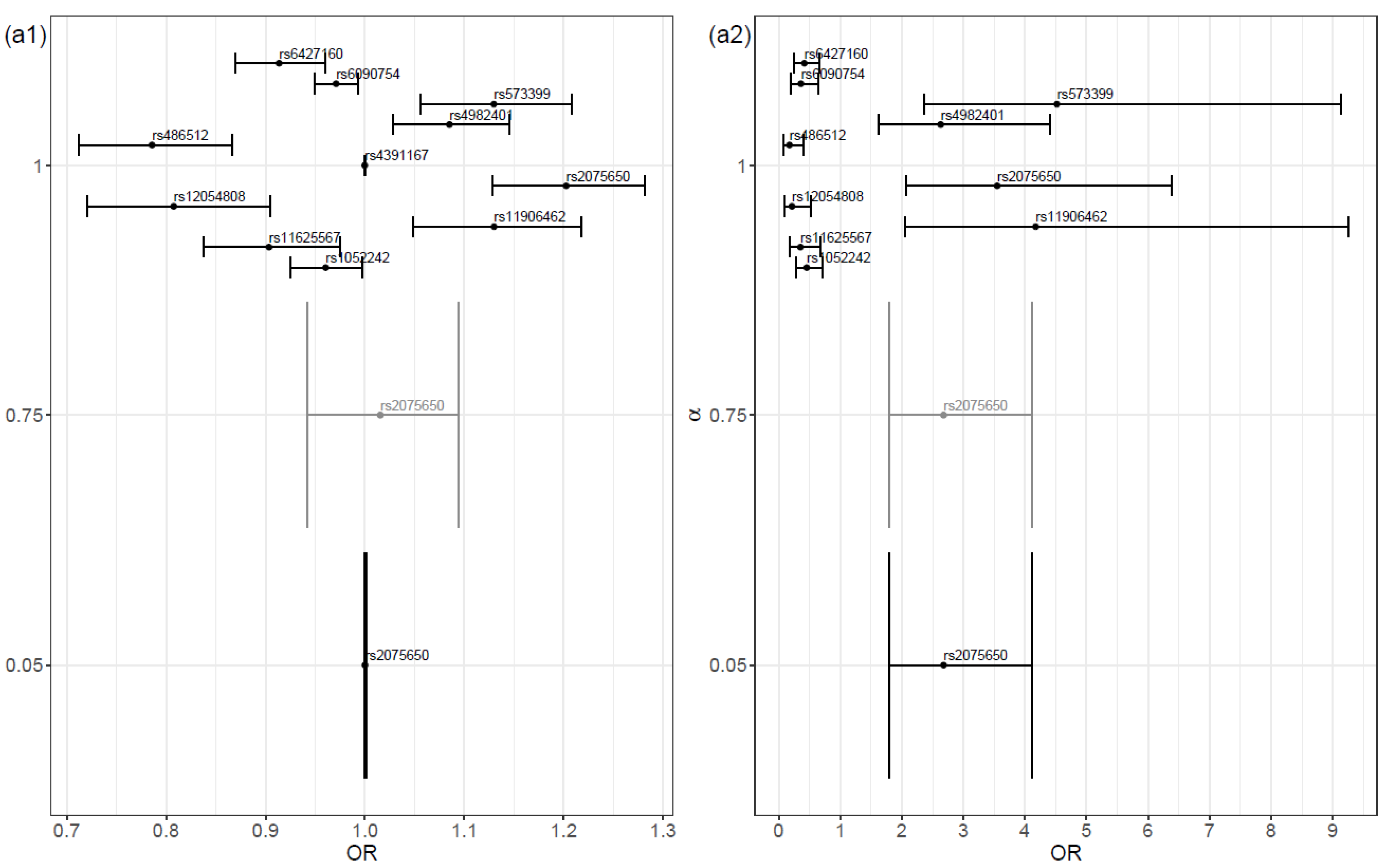
The magnitude of the coefficient estimates on the proposed models increased as the value of α increased. In general, as the alpha value increased, the odds ratio deviated further from the value 1 (
Figure 2(a1,b1)). A high similarity existed between the selected variables in both scenarios. The main difference was that the model fitted in Scenario SNPs + Cov contained the covariate
APOE4 genotype, instead of the SNPs
rs6090754,
rs1052242, and
rs4982401. Naturally, the magnitude of the coefficient estimates was higher in the α = 1 model and, consequently, the risk and protection effects were increased.
As expected, due to the shrinkage, the protective and risk effects were always lower in our approach than in the traditional logistic regression approach (
Figure 2).
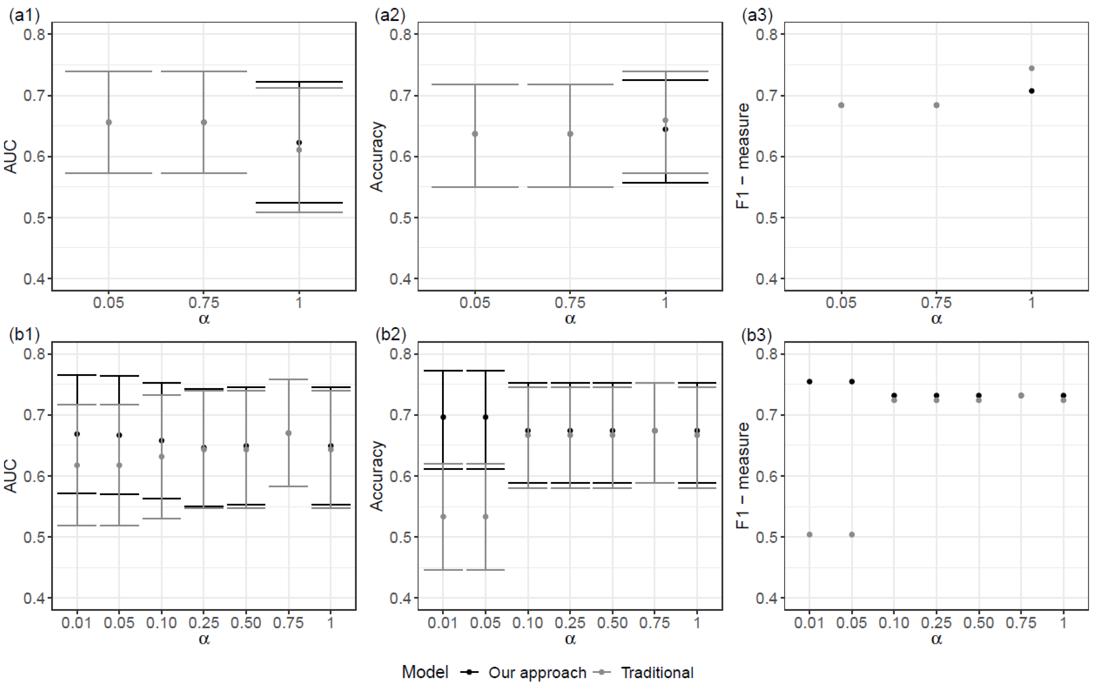
The bets performance for Scenario SNPs + Cov was achieved when α = 0.01. In the case of Scenario SNPs, an overall better result was achieved when α = 1 than for lower values of α. Overall, regression models defined for Scenario SNPs + Cov had a better performance than those for Scenario SNPs (
Figure 3).
When comparing the proposed model with the corresponding traditional logistic regression model, the performances were similar. In truth, the proposed models show a slightly better performance with higher values of the AUC and the F1-measure (
Figure 3). It should be noted that the traditional logistic regression model was obtained via the prior selection of variables and was achieved with the proposed approach.
4. Discussion
In this work, a stable variable selection method with shrinkage regression was proposed and applied to the ADNI public dataset. Based on the repeated applications of a penalized regression model, we designed a procedure that measured the relative importance of each selected variable via the combination of the results of all the penalized regression models. Through its design, the procedure highlights the most commonly selected variables, giving greater emphasis to the ones selected in the models that best fit the data. Since the proposed procedure is more restrictive than the usual correspondent penalized regression approach, stability is favored during variable selection.
The penalized regression models were constructed using LASSO (α = 1) and Elastic-Net (0 < α < 1) methods for α values in the grid {0.75, 0.50, 0.25, 0.10, 0.05, 0.01}. The alpha parameter controls the balance between the L1 and L2 regularization penalties; α = 1 forces some variable’ coefficients to be equal to zero, thus leading to a smaller number of selected predictors; and, in general, the number of selected variables increases as the α value decreases.
For each specific value of , a large dispersion in the number of selected variables was observed in relation to the 100 penalized regression models. The designed procedure allowed us to overcome this instability by defining a single set of predictor variables which were restricted to the most important variables across all the penalized models.
In analyzing the final models across the α values, differences were found in the set of the selected variables. A more in-depth analysis showed that the variables’ rank by their weights, as defined in step 2, is the same across all α values. This means that some variables were not flagged as important due to the restrictive cutoff value (defined as 0.8), and, therefore, they were not included in the final model. The lack of consistency between the α models can be overcome via adjusting the threshold value for the α parameter.
As expected, for each fixed α, there were differences between scenarios with and without the inclusion of the covariates age, sex, educational level, and
APOE4 genotype (Scenario SNPs and Scenario SNPs + Cov, respectively). In general, the results were consistent for the common SNPs of the two scenarios proposed; the significance of the coefficients and the effects of the variables (risk or protection) remained the same (
Figure 2(a1,b1)). The same was verified in relation to the corresponding traditional logistic regression model.
When analyzing the predictors selected by our procedure in greater detail, particularly those observed for higher α values, and when comparing these results with the literature, some interesting results emerge. Both the SNP
rs2075650 and the
APOE4 genotype are referenced in the literature as risk factors for AD [
18,
19]. The first factor was selected for our procedure in both scenarios (Scenario SNPs and Scenario SNPs + Cov). The OR estimates obtained by the proposed procedure were, as expected, lower than those obtained with the traditional regression procedure both in this work and in the literature (e.g., in reference [
18], OR = 4.178 and 95% CI 1.891–9.228). The second risk factor mentioned above, the
APOE4 genotype, was also selected in the construction Scenario SNPs + Cov regression model.
In addition, the SNPs rs573399 and rs11906462 were identified as important variables in the two scenarios and, in both cases, as risk factors for AD. Also, rs12054808 and rs486512 were selected consistently with an odds ratio less than one, which indicates an anticipated protective effect for AD. These SNPs were not found to be associated with AD in the literature. Since the proposed variable selection procedure is more restrictive than the usual correspondent penalized regression approach, we believe that the selected variables have potential to be tested as genetic predictors of AD.
The proposed procedure for feature selection can thus be advantageously applied to other contexts where a very high number of predictors exist in relation to the number of individuals under study. It is well known that, in such contexts, the usual feature selection methods are unstable, i.e., the same dataset yielding distinct results. Our results demonstrate the potential of this new procedure to overcome this issue, outperforming other methods in terms of the stability of variable selection.


 ,
, 
 language was used to carry out the statistical analysis.
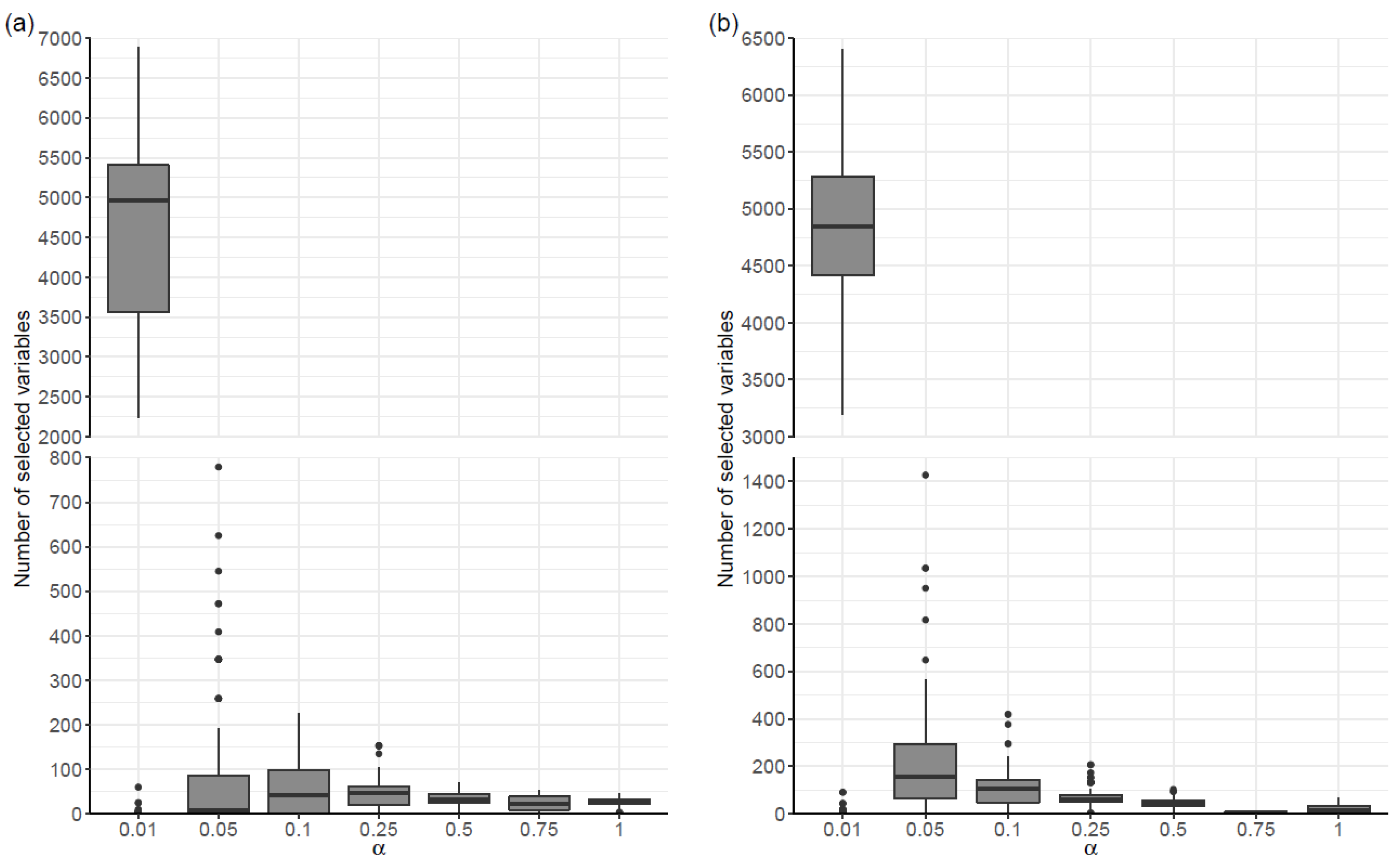

