Pointwise Nonparametric Estimation of Odds Ratio Curves with R: Introducing the flexOR Package

Abstract

The analysis of odds ratio curves is a valuable tool in understanding the relationship between continuous predictors and binary outcomes. Traditional parametric regression approaches often assume specific functional forms, limiting their flexibility and applicability to complex data. To address this limitation and introduce more flexibility, several smoothing methods may be applied, and approaches based on splines are the most frequently considered in this context. To better understand the effects that each continuous covariate has on the outcome, results can be expressed in terms of splines-based odds ratio (OR) curves, taking a specific covariate value as reference. In this paper, we introduce an R package, flexOR, which provides a comprehensive framework for pointwise nonparametric estimation of odds ratio curves for continuous predictors. The package can be used to estimate odds ratio curves without imposing rigid assumptions about their underlying functional form while considering a reference value for the continuous covariate. The package offers various options for automatically choosing the degrees of freedom in multivariable models. It also includes visualization functions to aid in the interpretation and presentation of the estimated odds ratio curves. flexOR offers a user-friendly interface, making it accessible to researchers and practitioners without extensive statistical backgrounds.

1. Introduction

Logistic regression models [1] serve as powerful tools in statistical analysis, particularly when the outcome variable is binary. In contrast to linear regression, which is tailored for continuous dependent variables, logistic regression is specifically crafted for predicting the probability of an event, making it particularly applicable to scenarios like estimating the likelihood of a patient developing coronary disease or experiencing a specific medical outcome. Within logistic regression, addressing the nonlinear effects of continuous predictors is a pivotal challenge, as conventional models may lead to substantial errors. To address this issue, two conventional approaches have historically been employed: (i) categorizing predictors, creating dummy variables, and calculating the effects considering an appropriate reference category; or (ii) the incorporation of these predictors into a polynomial model. The categorical approach provides averaged effects for each category, posing the challenge of determining the optimal number of categories and the appropriate placement of their cutpoints [2]. As we delve into the existing literature, numerous methods for determining appropriate cutpoints have been proposed [3,4]. These approaches aim to mitigate the subjectivity associated with cutpoint selection, offering a systematic means for investigators. However, it becomes evident that this strategy falls short of resolving two critical issues: the potential loss of statistical power and the reliance on averaged risks within predefined categories when estimating relative risks or odds ratios. Consequently, there arises a need for innovative approaches that not only address the nonlinearity in continuous predictors but also tackle the inherent challenges of cutpoint determination, power loss, and the impact on risk estimation.

The utilization of polynomial regression has been a common practice to address the challenges posed by nonlinear effects in continuous predictors. Polynomial regression allows for the inclusion of higher-order terms, providing a flexible framework to capture complex nonlinear patterns in the data. However, despite its versatility, polynomial regression has limitations, including susceptibility to overfitting and difficulties in interpretation. In response to these challenges, generalized additive models (GAMs) [5,6] offer an alternative solution that take in consideration the incorporation of nonlinear forms for the explanatory variables. GAMs, particularly those employing spline regression and smoothing splines, enhance the capacity to model nonlinear effects more effectively. Splines provide a flexible way to represent nonlinear relationships by dividing the predictor space into smaller intervals and fitting separate polynomials to each segment, mitigating the risk of overfitting associated with high-order polynomials.

Smoothing splines are a popular technique for fitting a smooth curve to data while balancing between goodness-of-fit and smoothness. Let $f\left(x\right)$ be the function we aim to estimate, and let $y_i$ be the observed response corresponding to predictor variable $x_i$. The goal is to find the function $f\left(x\right)$ that minimizes the following penalized residual sum of squares (RSS):

$$\mathrm{RSS}(f,\lambda )=\sum _{i=1}^n{(y_i-f\left(x_i\right))}^2+\lambda \int {\left[f^{″}\left(t\right)\right]}^{2}dt$$

where $\lambda$ is a fixed smoothing parameter controlling the trade-off between fit and smoothness. The first term measures the discrepancy between the observed and estimated values. The second term penalizes the roughness of the curve, where $f^{″}\left(x\right)$ is the second derivative of $f\left(x\right)$.

The minimization problem can be solved by expressing $f\left(x\right)$ as a piecewise polynomial function with knots at predetermined points. Within each interval between knots, $f\left(x\right)$ is represented by a polynomial of degree d, resulting in a set of equations. To ensure smoothness at knot points, additional constraints are imposed on the derivatives of adjacent polynomials.

The final estimated function is a smooth curve that passes through the data points while minimizing roughness. By adjusting $\lambda$ and the placement of knots, the degree of smoothing can be controlled, allowing flexibility in capturing complex relationships in the data. For further insights, additional details can be found in [5] or [7].

A drawback associated with employing splines or smoothing splines to model the effect of a continuous covariate lies in the challenge of selecting the number and placement of knots that define the smooth line. The arbitrary determination of these parameters may inadvertently obscure crucial features in the dataset. Striking the right balance is essential, as an excessive number of knots can result in oversmoothing, while too few can lead to undersmoothing. Some implementations, such as the gam package in R, automatically select the number and position of knots based on the data and the specified degrees of freedom for the smoother. Various methods have been proposed to address this issue, with one approach relying on minimizing Akaike’s Information Criterion (AIC, [8]), and an alternative based on minimizing a corrected version thereof (AICc, [9]). While these criteria are straightforward to minimize in a univariate context, their application becomes more intricate in multivariable settings. The Bayesian Information Criterion (BIC), initially proposed by [10] presents another viable option in this context.

In response to these challenges, we introduce the flexOR package, accessible on the Comprehensive R Archive Network at https://CRAN.R-project.org/package=flexOR (accessed on 27 April 2024). This package offers a methodological advancement by incorporating robust nonparametric methods that improve the modeling and interpretation of odds ratios (ORs) within logistic regression frameworks.

The conceptual foundations of this approach draw inspiration from the work of [11,12], who introduced a versatile method for constructing hazard ratio curves with confidence limits. This methodology, rooted in clinical survival studies, leverages an additive Cox model where the nonlinear effects of continuous predictors on log hazards are elegantly modeled using P-splines. In our context, our objective is to estimate the odds ratios (OR) and their associated confidence intervals through a nonparametric approach. However, as in [11,12] we aim to estimate these curves while considering a reference value. Capitalizing on the asymptotic normality of the logarithm of the odds ratio, we employ a new approximation for the covariance matrix of the log-odds ratio to construct these confidence intervals.

One of the cornerstones of flexOR is the dfgam function, which determines the optimal number of degrees of freedom for smoothing in multivariable additive logistic models. The optimal degree of smoothing is ascertained by minimizing any of the following criteria: AIC, AICc, or BIC. The AIC is a measure of the relative quality of statistical models, balancing goodness of fit and model complexity. The AICc is a corrected version of AIC, particularly useful in situations with a limited sample size to prevent overfitting. Researchers often use these criteria to guide model selection, and in the context of smoothing parameters, they provide a systematic way to balance model fit and complexity. In addition, dfgam also incorporates the restricted maximum likelihood method (REML) and generalized cross-validation (GCV) into the implemented methods with a particular emphasis on the GCV.Cp criterion, as implemented in the famous mgcv package [6]. The use of these methods is particularly relevant in models involving multiple covariates with nonlinear effects, ensuring that the selected model is optimally adjusted without being overfitted or underfitted.

The practical implications of flexOR are important, particularly in fields where precise modeling of continuous variables is crucial, such as epidemiology and biomedical research. By providing more accurate and interpretable models, this package aids in the clear understanding of risk factors and their interactions. Additionally, flexOR offers detailed graphical and numerical outputs, including adjusted OR curves and confidence intervals while considering a reference value, enhancing the interpretability of logistic regression results in research and clinical settings.

The remainder of this paper is organized as follows: Section 2 discusses the theoretical background and the statistical methods underlying the flexOR package. Section 3 details the software implementation and functionality, followed by Section 4, which presents a case study demonstrating the application of flexOR. Finally, Section 5 concludes with a discussion of the results and potential future directions for this research.

2. The Additive Model

Logistic regression is a widely used statistical method for modeling the probability of a binary outcome. The logistic regression model is based on the logistic function, and it expresses the log-odds of an event as a linear combination of predictor variables. The logistic function is defined as

$$p\left(x\right)=\frac{e^{{\beta }_0+{\beta }_1{x}_1+{\beta }_2{x}_2+\dots +{\beta }_p{x}_p}}{1+e^{{\beta }_0+{\beta }_1{x}_1+{\beta }_2{x}_2+\dots +{\beta }_p{x}_p}}$$

(1)

where $p\left(x\right)=p(Y=1|X=x)$ is the probability of the event, ${\beta }_0$ is the intercept term, and ${\beta }_i$, $1\le i\le p$ are the coefficients of the predictor variables $X_i$.

The log-odds (logit) of the event is given by

$$ln\left(\frac{p\left(x\right)}{1-p\left(x\right)}\right)={\beta }_0+{\beta }_1{x}_1+{\beta }_2{x}_2+\dots +{\beta }_p{x}_p$$

(2)

The odds ratio (OR) in logistic regression is a crucial measure of association between a predictor variable and the outcome. The adjusted OR for a subject with (continuous) covariate value $X_i=x_i$ compared with a subject with covariate value $x_{i,ref}$ is given by

$$\mathrm{OR}(x_i,x_{i,ref})=exp\left({\beta }_i(x_i-x_{i,ref})\right)$$

(3)

In its additive form, the logistic additive model expresses the log-odds of an event that can be written as

$$ln\left(\frac{p\left(x\right)}{1-p\left(x\right)}\right)={\beta }_0+\sum _{i=1}^q{\beta }_i{x}_i+\sum _{i=q+1}^p{f}_i\left(x_i\right)$$

(4)

where the first q covariates are introduced parametrically in the model and the remaining ones are introduced nonlinearly through (unknown) smooth functions, $f_i$.

Model (4) stands out as particularly well-suited for various applications due to its ability to accommodate nonlinear, smooth effects for continuous predictors, thereby providing a substantial increase in flexibility. These effects can be effectively modeled using regression splines [13] or smoothing splines [5]. Assuming (4), the adjusted odds ratio for a subject with covariate value $X_i=x_i$, $i>q$ compared with a subject with covariate value $x_{i,ref}$ is given by

$$\mathrm{OR}(x_i,x_{i,ref})=\frac{exp\left(f_i\left(x_i\right)\right)}{exp\left(f_i\left(x_{i,ref}\right)\right)}=exp(f_i\left(x_i\right)-f\left(x_{i,ref}\right))$$

(5)

A critical decision in estimating the function $f\left(x\right)$ is the selection of the smoothing level, which directly influences the smoothness of the estimated function $\widehat{f}\left(x\right)$. The Akaike Information Criterion (AIC), introduced by Akaike [8], and the Bayesian Information Criterion (BIC), proposed by Schwarz [10], stand out as widely utilized criteria for model selection in a given dataset. Grounded in log-likelihood (LogLik), these criteria can assist in determining the optimal model. For additive logistic models, selecting the appropriate level of smoothing is achieved by comparing models with varying degrees of freedom and opting for the one with the lowest AIC or BIC scores. The AIC, AICc, and BIC scores are calculated as follows:

$$\mathrm{AIC}=-2\times \mathrm{LogLik}+2\times k$$

$$\mathrm{BIC}=-2\times \mathrm{LogLik}+log\left(n\right)\times k$$

$$\mathrm{AICc}=\mathrm{AIC}+2\times k(k+2)/(n-k-1)$$

where LogLik is the log-likelihood of the fitted model, k represents the equivalent degrees of freedom of the model, and n is the number of observations in a given dataset.

The implementation of AIC, BIC, and AICc criteria to determine the degree of smoothing for the corresponding continuous variable is straightforward for the case of a model with a single covariate with a nonlinear effect, using one of these approaches. However, it will entail fitting and comparing a large number of models. If we aim to fit a larger number of covariates, this approach is no longer as simple. Later on, we illustrate the application of these methods to real data, where we apply them to three covariates, for which we propose using the dfgam function developed by us. This function utilizes an iterative process, starting from an initial value for the smoothing degree, and through three or more steps, we arrive at a value for the smoothing degree in the covariates adjusted in the model.

Within the mgcv R package for GAMs, the estimation of smoothing parameters is achieved by maximizing the Restricted Maximum Likelihood (REML) score. The REML score is intricately connected to the model likelihood augmented by a penalty term. The likelihood term is contingent upon the distributional assumption of the response variable, such as binomial for binary responses. On the other hand, the penalty term encompasses the smoothing parameters associated with the smooth terms embedded in the model.

The method “GCV.Cp” in package mgcv uses GCV for unknown scale parameters and Mallows’ Cp/UBRE/AIC for known scale. The GCV formula for a GAM is the following:

$$\mathrm{GCV}=\frac{1}{n}\sum _{i=1}^n{\left(\frac{y_i-\widehat{f}\left(x_i\right)}{1-\mathrm{trace}\left(\mathbf{S}\right(\lambda \left)\right)/n}\right)}^2$$

where $\lambda$ is the smoothing parameter that controls the amount of smoothing, n is the number of observations, $y_i$ is the observed response for the i-th observation, $\widehat{f}\left(x_i\right)$ is the predicted value for the i-th observation and $\mathbf{S}\left(\lambda \right)$ is the smoother matrix associated with the penalty parameter $\lambda$.

The GCV criterion seeks to balance model fit and complexity by penalizing the model for the number of parameters estimated. REML and GCV.Cp are optimization problems. We utilize the mgcv package, which, in turn, employs numerical optimization techniques to determine optimal values for smoothing parameters. These values are obtained by either maximizing the REML score or minimizing the GCV.Cp criterion. The REML may exhibit a higher susceptibility to oversmoothing, and the choice among these methods depends on the specific characteristics and requirements of the data and modeling context.

The criteria, implemented in the package, encompass Restricted Maximum Likelihood (REML) and a method known as GCV.Cp. GCV.Cp employs Generalized Cross-Validation (GCV) when dealing with an unknown scale parameter or an UnBiased Risk Estimator (UBRE) for a known scale parameter. UBRE essentially corresponds to a scaled AIC in the generalized case or Mallows’ Cp in the additive model case. The REML approach aims to maximize the restricted likelihood of the model given the data, while GCV.Cp strives to strike a balance between the goodness of fit and the complexity of the model.

It is important to note that, in our case, the confidence bands for the odds ratio ($\widehat{\mathrm{OR}}(x_i,x_{i,ref})$) are obtained considering a reference value that always needs to be defined by the user, unless predefined values such as minimum or maximum are used. Therefore, the graphical representations obtained will be different from those provided by other tools currently available, such as those found in the gam or mgcv libraries of the R software (version 4.4.0).

The asymptotic variance of Ln$\widehat{\mathrm{OR}}(x_i,x_{i,ref})$ can be expressed in terms of the covariance matrix of the smoother ${\widehat{f}}_i\left(x_i\right)$: $Var\left(\mathrm{Ln}\widehat{\mathrm{OR}}(x_i,x_{i,ref})\right)=Var\left({\widehat{f}}_i\left(x_i\right)\right)+Var\left({\widehat{f}}_i\left(x_{i,ref}\right)\right)-2Cov({\widehat{f}}_i\left(x_i\right),{\widehat{f}}_i\left(x_{i,ref}\right))$.

Following Hastie and Tibshirani [5,14], the estimate ${\widehat{f}}_i\left(x_i\right)$ can be given by ${\widehat{f}}_i\left(x_i\right)=S·z\left(x_i\right)=(H+G)·z\left(x_i\right)=H·z\left(x_i\right)+G·z\left(x_i\right)=\widehat{\theta }{x}_i+\widehat{g}\left(x_i\right)$ In our context, the matrix S represents the (weighted) smoother matrix applied to the working response $z\left(x_i\right)$, which is obtained from the Fisher Scoring fit. Specifically, the S matrix we typically consider is based on cubic smoothing splines. This matrix S is orthogonally decomposed into a sum of two matrices: H and G. Here, H serves as the projection operator matrix, providing an estimate of the corresponding parametric part of $f_i\left(x_i\right)$, while G acts as the non-projection operator matrix, responsible for smoothing $g_i\left(x_i\right)$ using cubic smoothing splines.

From this, we can rewrite the corresponding asymptotic variance as follows:

$$\begin{array}{c}Var\left(\mathrm{Ln}\widehat{\mathrm{OR}}(x_i,x_{i,ref})\right)=\widehat{\varphi }{(x_i-x_{i,ref})}^{2}Var\left(\widehat{\theta }\right)+Var\left({\widehat{g}}_i\left(x_i\right)\right)+Var\left({\widehat{g}}_i\left(x_{i,ref}\right)\right)\hfill \\ \hfill -2Cov({\widehat{g}}_i\left(x_i\right),{\widehat{g}}_i\left(x_{i,ref}\right))\end{array}$$

where $\widehat{\varphi }$ is the estimated dispersion parameter $\varphi$ of the model, and $Cov\left({\widehat{g}}_i\right)$ represents the asymptotic covariance matrix of the purely nonparametric smoother function ${\widehat{g}}_i\left(x_i\right)$.

Given that the two components, $\widehat{\theta }{x}_i$ and ${\widehat{g}}_i\left(x_i\right)$, of the smoother ${\widehat{f}}_i\left(x_i\right)$ are shown to follow asymptotically a normal distribution, we finally have that $\mathrm{Ln}\widehat{\mathrm{OR}}(x_i,x_{i,ref})\sim N\left(\mathrm{Ln}\mathrm{OR}(x_i,x_{i,ref})\right),Var\left(\mathrm{Ln}\widehat{\mathrm{OR}}(x_i,x_{i,ref})\right)$.

3. Software Description

The flexOR R package is designed to generate pointwise estimates of OR curves for continuous predictors along with their corresponding confidence limits. Integrated seamlessly with the R statistical environment [15], this package includes a suite of functions that support both numerical analysis and graphical representation.

Table 1. Summary of functions in the flexOR package.

Function	Description
AICc	Calculates AICc, the Akaike Information Criterion corrected for small sample sizes, for Generalized Additive Models.
floor_to	Takes a numeric value or vector and rounds it down to the nearest multiple of a specified base.
dfgam	Calculates the degrees of freedom for specified non-linear predictors in a GAM model.
flexOR	Computes odds ratios and CIs for predictors in GAM models.
plot.OR	Plots smooth odds ratios along with confidence intervals for a specified predictor. For an object of class OR.
predict.OR	Predicts values using a fitted OR model.

provides a summary of the available functions. Detailed guidance on using these functions can be found in the respective help pages.

Managing the level of smoothing in additive models is particularly challenging, especially in multivariable contexts. To address this, we introduce the dfgam function, which allows flexible control over the degree of smoothing by providing various methodological options for optimization. In its current implementation, the dfgam function exclusively supports the “s” option for the smoother parameter, which indicates the use of smoothing splines for modeling nonlinear effects of predictors.

        
	  dfgam(
	   response,
	   nl.predictors,
	   other.predictors = NULL,
	   smoother = "s",
	   method = "AIC",
	   data,
	   step = NULL
	  )
	  
      

This function requires continuous predictors that need to be introduced nonlinearly to be specified in the nl.predictors argument (as a vector), using smoothing splines (smoother = “s”), while other predictors (continuous or not) are included under other.predictors. This function generates a list containing the degrees of freedom for the spline smoothing terms, determined by the minimization of specific criteria based on the selected method. These criteria include (a) the Akaike Information Criterion (AIC) when method=“AIC”, (b) a variant of the corrected AIC, adapted from [9], when method=“AICc”, (c) the Bayesian Information Criterion (BIC) when method=“BIC”, (d) the restricted maximum likelihood (REML) score when method=“REML”, and (e) the Generalized Cross-Validation Criterion plus a penalty (GCV.Cp) when method=“GCV.Cp”.

The flexOR function, the cornerstone of the package, requires data, a response variable, and a formula to compute the odds ratios:

        
	  flexOR(
	   data,
	   response,
	   formula
	  )
	  
      

The plot function can then visualize flexible odds ratio curves, accommodating nonlinear relationships between continuous predictors and the response variable:

        
	  plot(
	   x,
	   predictor,
	   prob = NULL,
	   ref.value = NULL,
	   conf.level = 0.95,
	   round.x = NULL,
	   ref.label = NULL,
	   col,
	   main,
	   xlab,
	   ylab,
	   lty,
	   xlim,
	   ylim,
	   xx,
	   ylog = TRUE,
	   ...
	  )
	  
      

The reference value is set using the ref.value argument or determined automatically to represent either the minimum or maximum of the odds ratio curve, depending on the setting of the prob argument.

Users are encouraged to utilize the output of flexOR with additional R packages such as plotly for creating more interactive and dynamic visualizations. This integration not only enhances the interpretative value of the statistical analysis but also provides a more engaging way to explore the data visually. Details on generating interactive plots using the plotly R package and the application of these advanced functions will be demonstrated in subsequent sections, using two real datasets.

4. Examples of Application

This section demonstrates the application of the flexOR package integrated with the R statistical program [15]. Here, we illustrate the functionality of the package through analyses conducted on two real datasets. The first dataset involves a reanalysis of data from 811 patients admitted with acute coronary syndrome (ACS) to the Santiago University Teaching Hospital between September 2003 and March 2007. A primary objective of this study is to evaluate the predictive power of fasting blood glucose levels alongside other variables within this dataset.

The second dataset considered is collected by the US National Institute of Diabetes and Digestive and Kidney Diseases, focusing on a cohort of women aged 21 and above, of Pima Indian heritage, residing near Phoenix, Arizona. This dataset, available in the mlbench package of R, is commonly used to predict the likelihood of diabetes based on specific diagnostic measurements. It comprises 768 observations and includes variables such as age, plasma blood glucose, diastolic blood pressure, and body mass index, among others. Researchers utilize this dataset extensively to explore and develop predictive models for diabetes, leveraging the rich array of variables it offers.

4.1. Acute Coronary Syndrome Data

This study aims to assess and compare the predictive efficacy of fasting glucose in forecasting mortality among patients with acute coronary syndrome (ACS). The analysis involves modeling the intricate, nonlinear relationships between glucose levels and the risk of death, utilizing smoothing splines within the framework of additive logistic regression.

To explore the intricate dynamics of mortality prediction, a Generalized Additive Model (GAM) was employed. This model considered the binary response variable “exitus” (death) and incorporated key predictors, including age, creatinine, fasting blood glucose levels, anemia, sex, and smoking status (nonsmoker, smoker, and ex-smoker).

Specifically, nonlinear relationships for age (years), creatinine, and fasting glucose levels were modeled using smoothing splines. The degrees of freedom for the smooth terms were determined using the dfgam function, minimizing the AIC criterion. The resulting degrees of freedom were 8.9 for age, 1.8 for creatinine, and 4.6 for fasting. In this case, to obtain the degrees of freedom for the three covariates, the dfgam function started with an initial value provided by the REML method, and through a recursive three-step process (default value, step = 3), it obtained the respective degrees of freedom for the three covariates.

All selected predictors—age, creatinine, and fasting—demonstrated statistically significant effects, with their respective smooth terms exhibiting significant F-values. The model, fitted using the gam function from the gam R library, also captured the influence of anemia, sex, and smoking status, the first and the last showing significant effects.

The overall model fit was evaluated through the analysis of deviance, indicating a strong fit to the data. These findings underscore the crucial role of the specified predictors in predicting the binary response outcome (death).

          
		> library ("flexOR")
		> df1 <- dfgam(response="exitus",
		    nl.predictors=c("age","creatinine","fasting"),
		    other.predictors=c("anemia","sex","smoking"),
		    smoother="s",
		    method="AIC",
		    data = heart2)
		> df1$df
		        df
		age      8.9
		creatinine   1.8
		fasting    4.6
		> m1 <- gam(exitus ~ s(age, 8.9) + s(creatinine, 1.8) + s(fasting, 4.6) +
		        anemia + sex + factor(smoking),
		        data=heart2,
		        family=binomial())
		> summary(m1)
		Anova for Parametric Effects
		             Df Sum Sq Mean Sq F value  Pr(>F)
		s(age, 8.9)      1.0  43.44  43.444 49.9012 3.548e-12 ***
		s(creatinine, 1.8)   1.0  16.08  16.077 18.4669 1.944e-05 ***
		s(fasting, 4.6)    1.0  10.71  10.709 12.3004 0.0004784 ***
		anemia         1.0  15.69  15.693 18.0257 2.438e-05 ***
		sex           1.0   2.71   2.713  3.1165 0.0778910 .
		factor(smoking)     2.0   7.44   3.720  4.2725 0.0142708 *
		Residuals       790.7  688.38   0.871
		---
		Signif. codes:  0 ‘***’ 0.001 ‘**’ 0.01 ‘*’ 0.05 ‘.’ 0.1 ‘ ’ 1
		     
		Anova for Nonparametric Effects
		             Npar Df Npar Chisq  P(Chi)
		(Intercept)
		s(age, 8.9)         7.9    21.6053 0.005358 **
		s(creatinine, 1.8)      0.8    3.2991 0.050784 .
		s(fasting, 4.6)       3.6    9.3431 0.040178 *
		anemia
		sex
		factor(smoking)
		
        

The most effective means of interpreting the nonlinear effects is through the analysis of the corresponding plot. Below, we present the input commands to generate the log-odds ratio curve illustrating the relationship between the odds of death and fasting glucose among ACS patients. The resulting plot is showcased in Figure 1. The figure illustrates a spoon-shaped dependence of the mortality odds ratio on fasting glucose, with the lowest odds observed at 114 mg/dL (6.3 mmol/L; to convert mg/dL of glucose to mmol/L, divide by 18). The log-odds ratio (LnOR) is visually represented, accompanied by 80% (depicted in gray) and 95% (light gray) confidence bands, utilizing a reference value of 100 for fasting blood glucose. Users have the option to choose a single confidence level, although two are also feasible, as demonstrated in the input command below. Additionally, the argument “ylog” provides the flexibility to generate a plot that is not on the log scale.

          
		> or1 <- flexOR(data = heart2, response = "exitus",
		     formula = ~s(age, 8.9) + s(creatinine, 1.8) + s(fasting, 4.6) +
		     anemia + sex + factor(smoking))
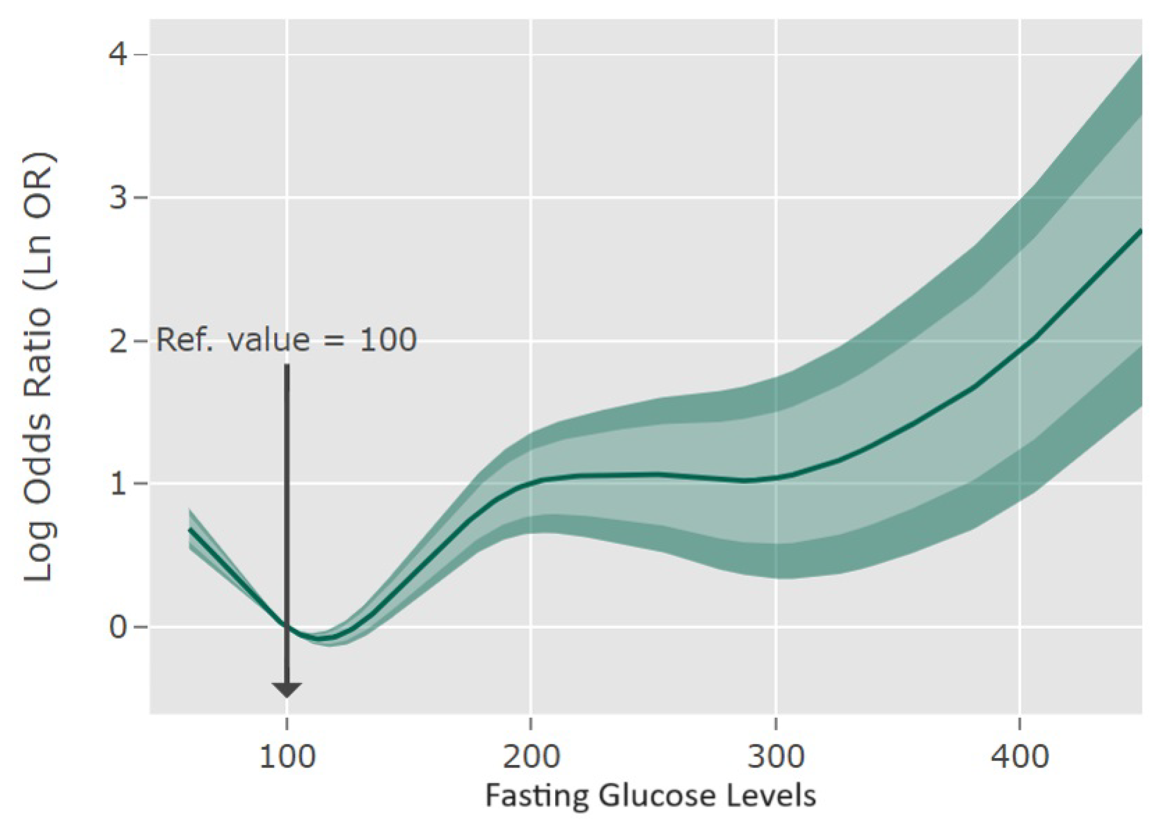
		> plot(
		  x = or1,
		  predictor = "fasting",
		  ref.value = 100,
		  ref.label = "Ref. value",
		  col.area = c("grey75", "grey90"),
		  main = " ",
		  xlab = "Fasting blood glucose levels",
		  ylab = "Log Odds Ratio (Ln OR)",
		  lty = c(1,2,2,3,3),
		  ylog = TRUE,
		  round.x = 1,
		  conf.level = c(0.8, 0.95)
		)
		
        

Plotly’s R graphing library offers a powerful tool for creating interactive, publication-quality graphs that enhance data visualization experiences. The library’s versatility allows users to go beyond static representations and delve into dynamic visualizations, enabling a more engaging exploration of the data. In the example provided, the input commands showcase the library’s capability to generate a smoothed log-odds curve with two confidence bands. The interactive nature of these plots facilitates a deeper understanding of the underlying patterns by allowing users to zoom in, pan, and hover over data points for detailed insights. This interactivity not only enhances the overall user experience but also promotes a more nuanced and insightful interpretation of the graphed information. Below are the input commands, along with the corresponding Figure 2.

          
		> library(plotly)
		 
        > p <- plot(
          x = or1,
          predictor = "fasting",
          ref.value = 100,
          ref.label = "Reference Label",
          main = "Smooth odds ratio for Fasting blood glucose",
          xlab = "Fasting blood glucose levels",
          ylab = "Log Odds Ratio (Ln OR)",
          lty = c(1,2,2,3,3),
          xlim = c(60, 450),
          round.x = 1,
          conf.level = c(0.8, 0.95)
        )
		 
        > tmat <- p$estimates
        > xref <- p$xref
        > mdata <- or1$dataset
        > jj <- match(sort(unique(mdata$fasting)), mdata$fasting)
		 
        # Plotly to get shaded (two-levels) confidence bands
        > fig <- plot_ly(x=mdata$fasting[jj], y=tmat[jj,5],
                   type = ’scatter’, mode = ’lines’,
                   line = list(color = ’transparent’),
                   showlegend = FALSE, name = ’80%UCI’)
        > fig <- fig %>% add_trace(y = ~tmat[jj,3], type = ’scatter’,
        mode = ’lines’,
                   fill = ’tonexty’, fillcolor = ’rgba(0,100,80,0.3)’,
                   line = list(color = ’transparent’),
                   showlegend = FALSE, name = ’95%UCI’)
        > fig <- fig %>% add_trace(y = ~tmat[jj,2], type = ’scatter’,
        mode = ’lines’,
                   fill = ’tonexty’, fillcolor=’rgba(0,100,80,0.3)’,
                   line = list(color = ’transparent’),
                   showlegend = FALSE, name = ’95%LCI’)
        > fig <- fig %>% add_trace(y = ~tmat[jj,4], type = ’scatter’,
        mode = ’lines’,
                   fill = ’tonexty’, fillcolor=’rgba(0,100,80,0.3)’,
                   line = list(color = ’transparent’),
                   showlegend = FALSE, name = ’80%LCI’)
        > fig <- fig %>% add_trace(y = ~tmat[jj,1], type = ’scatter’,
        mode = ’lines’,
                   line = list(color=’rgb(0,100,80)’),
                   showlegend = FALSE, name = ’LnOR’)
        > fig <- fig %>% add_annotations( x = xref,
                   y = floor_to(min(tmat[jj,]), to=0.5),
                   xref = "x", yref = "y",
                   axref = "x", ayref = "y",
                   text = paste("Ref. value =",xref),
                   showarrow = T,
                   ax = xref,
                   ay = max(tmat[jj,])/2)
        > fig <- fig %>% layout(#title = "",
                  plot_bgcolor=’rgb(229,229,229)’,
                  xaxis = list(title = "Fasting glucose levels",
                      gridcolor = ’rgb(255,255,255)’,
                      showgrid = TRUE,
                      showline = FALSE,
                      showticklabels = TRUE,
                      tickcolor = ’rgb(127,127,127)’,
                      ticks = ’outside’,
                      zeroline = FALSE),
                  yaxis = list(title = "Log Odds Ratio (Ln OR)",
                      gridcolor = ’rgb(255,255,255)’,
                      showgrid = TRUE,
                      showline = FALSE,
                      showticklabels = TRUE,
                      tickcolor = ’rgb(127,127,127)’,
                      ticks = ’outside’,
                      #range = c(-0.5,3.5),
                      zeroline = FALSE))
		 
        > fig
		
        

Figure 1 and Figure 2 illuminate the intricate relationship between fasting blood glucose levels and the odds of death among Acute Coronary Syndrome (ACS) patients. The log-odds ratio (LnOR) is presented alongside 80% and 95% confidence bands, all referenced to a reference value of 100 for fasting blood glucose levels.

It is imperative to note that normal fasting blood glucose concentrations typically fall within the range of 70 mg/dL (3.9 mmol/L) to 100 mg/dL (5.6 mmol/L). Notably, individuals with fasting blood glucose concentrations near 114 mg/dL exhibit a lower odds of death. The log-odds of death, as depicted in the figures, exhibits a distinctive spoon-shaped pattern, with a rapid escalation beyond this threshold until reaching a value of 200 mg/dL.

These findings shed light on the critical interplay between fasting blood glucose levels and mortality odds among ACS patients, emphasizing the nuanced nature of this relationship and its implications for clinical understanding and management.

Furthermore, it is important to highlight that both Figure 1 and Figure 2 present the same estimates while employing different plotting techniques. Figure 1 utilizes the conventional plotting method, while Figure 2 leverages the plotly R package.

The utilization of the plotly R package in Figure 2 introduces notable advantages, particularly its dynamic and interactive visualization capabilities. Plotly enables real-time interactivity, allowing users to explore the data in loco—providing a more immersive and detailed understanding of the fasting blood glucose level and its association with the odds of death among ACS patients. The incorporation of such interactivity improves the interpretability and utility of the presented findings in a practical and user-friendly manner.

It is important to note that while the functional form of the odds ratio (OR) for a particular predictor remains consistent regardless of the chosen reference point, the actual values of the odds ratio can be influenced by the selection of this reference point. This consideration must be taken into account when interpreting OR values.

The flexOR package also enables users to generate predictions based on the object or1 obtained from the flexOR function. The output provides predicted values along with confidence intervals for the log-odds ratio at different levels of the predictor variable fasting. The reference value is set at 100, and the confidence level is specified as 95%. The resulting table displays the reference value, log-odds ratios, and corresponding lower and upper bounds for the given prediction values.

          
		> pdval <- c (70, 80, 90, 100, 110, 120, 140, 180, 250, 400)
		> predict(or1, predictor = "fasting", ref.value = 100, conf.level = 0.95,
        prediction.values = pdval, ref.label = "Ref.")
		 
          Ref.      LnOR lower .95  upper .95
           70  0.48905582  0.3837869  0.59432470
           80  0.31326688  0.2430876  0.38344614
           90  0.14227425  0.1071846  0.17736388
          100  0.00000000  0.0000000  0.00000000
          110  -0.07323341  -0.1083230 -0.03814378
          120  -0.06143541  -0.1316147 0.00874384
          140  0.16943030  0.0290718  0.30978881
          180  0.81032300  0.5296060  1.09104001
          250  1.07569430  0.5493499  1.60203870
          400  1.89278576  0.8400970  2.94547454
		
        

Table 2. Degrees of freedom (df) for the multivariable logistic model with smoothing splines for age, creatinine, and fasting. The remaining variables were anemia, sex, and smoking. Acute coronary syndrome.

Covariates	AIC	GCV.Cp	REML
Age	8.9	6.97	3.34
Creatinine	1.8	1.79	2.06
Fasting	4.6	4.37	3.47

presents the degrees of freedom obtained for the multivariable logistic model incorporating smoothing splines for fasting, creatinine, and age, using data from acute coronary syndrome. Additional predictors in the model include anemia, sex, and smoking. The results indicate that the AIC-based method yields a higher number of degrees of freedom compared with GCV.Cp, particularly when compared with the REML method. Similar results were observed for AICc and BIC. The observed discrepancy between AIC and REML was anticipated, as the REML method may tend to oversmooth in certain instances. This disparity underscores the significance of choosing an appropriate method for determining degrees of freedom in additive logistic regression models. It has been confirmed that the scores obtained for the AIC criteria are lower for the logistic additive model with degrees of freedom derived through the AIC method.

4.2. Pima Indians Diabetes Database

In this Section 4.2 we use the Pima Indians Diabetes Database, a well-known dataset in the field of machine learning and statistics. The dataset originates from a study conducted by the National Institute of Diabetes and Digestive and Kidney Diseases (NIDDK) in the 1990s, focusing on the Pima Indian population in Arizona, USA.

The dataset includes various demographic, clinical, and diagnostic measurements for individuals, along with an indication of whether or not each person developed diabetes. Researchers and data scientists often use this dataset to develop and test predictive models for diabetes based on features like age (years), BMI (Body Mass Index), blood pressure, diabetes pedigree function, and other health-related variables. The dataset is available as part of the mlbench R package.

After identifying the variables to be included in the model and determining those requiring a nonlinear effect through smoothing splines, we utilized the dfgam function. This function enabled us to obtain optimal degrees of freedom, minimizing the AIC of the model. The resulting degrees of freedom for the nonlinear predictors, namely age and body mass index (mass), were determined to be 3.3 and 4.1, respectively. Subsequently, these optimal degrees of freedom were incorporated into the generalized additive model (GAM) using the gam function of the gam R package:

          
		> data(PimaIndiansDiabetes2, package="mlbench")
		> df2 <- dfgam(response="diabetes",
                     nl.predictors=c("age","mass"),
                     other.predictors=c("pedigree"),
                     smoother="s",
                     method="AIC",
                     data = PimaIndiansDiabetes2)
        > df2$df
           df
        age  3.3
        mass 4.1
        > m2 <- gam(diabetes ~ s(age, df=3.3) + s(mass, df=4.1) + pedigree,
              data=PimaIndiansDiabetes2, family=binomial)
		
        

Next, we can leverage the primary function of the flexOR package, which, in turn, is employed to generate a plot illustrating the smooth log-odds ratio curve. This curve, shown in Figure 3, provides insight into the relationship between the risk of diabetes and body mass index within the Pima Indian population in Arizona, USA. The log-odds ratio (LnOR) is visually represented, accompanied by 80% (depicted in gray) and 95% (light gray) confidence bands, using a reference value of 40 for BMI.

The input commands to generate the plot shown in Figure 3 are given below.

          
		> or2 <- flexOR(data = PimaIndiansDiabetes2,
                      response = "diabetes",
                      formula = ~s(age, 3.3) + s(mass, 4.1) + pedigree)
        > plot(
          x = or2,
          predictor = "mass",
          ref.value = 40,
          ref.label = "Ref. value",
          col.area = c("grey75", "grey90"),
          main = " ",
          xlab = "Body mass index",
          ylab = "Log Odds Ratio (Ln OR)",
          lty = c(1,2,2,3,3),
          round.x = 1,
          conf.level = c(0.8, 0.95)
        )
		
        

It is important to note that normal BMI values typically fall within the range of 19 to 25. In our context, individuals with a BMI lower than 40 manifest lower odds of diabetes. The log-odds of diabetes, as depicted in Figure 3, follows a distinctive pattern: there is a rapid increase until a BMI value of 30, followed by a relatively stable period between 30 and 40. However, beyond a BMI of 40, there is a notable and accelerated rise in the odds of diabetes.

Finally, the following input commands and results provide predicted values along with confidence intervals for the log-odds ratio at different levels of the predictor variable body mass index when a reference value is set at 40.

          
		> pdval <- c (20, 25, 30, 35, 40, 45, 50, 55, 60, 65)
        > predict(or2, predictor = "mass", ref.value = 40, conf.level = 0.95,
                   prediction.values = pdval, ref.label = "Ref.")
		 
          Ref.     LnOR  lower .95  upper .95
           20   -3.20826636 -3.7680373  -2.64849542
           25   -1.61356211 -2.0333903  -1.19373390
           30   -0.40263002 -0.6825155  -0.12274455
           35   -0.07505977 -0.2150025  0.06488297
           40  0.00000000  0.0000000  0.00000000
           45  0.45600760  0.3160649  0.59595034
           50  1.05087046  0.7709850  1.33075593
           55  1.63284725  1.2130190  2.05267546
           60  2.21353442  1.6537635  2.77330536
           65  2.83405429  2.1343406  3.53376797
		
        

Table 3. Degrees of freedom (df) for the multivariable logistic model with smoothing splines for age and mass. Pedigree was the remaining variable. Pima Indians diabetes.

Covariates	AIC	GCV.Cp	REML
Age	3.30	3.30	3.44
Mass	4.10	3.96	4.17

presents the degrees of freedom for the logistic model with smoothing splines for age and mass, and with pedigree as the additional predictor. In this case, the results show that all the methods provide similar results for the degrees of freedom.

5. Discussion

This paper provides a comprehensive overview of the flexOR package, showcasing its capabilities for computing pointwise estimates of odds ratio (OR) curves and corresponding confidence limits. Specifically designed for continuous predictors introduced nonlinearly in an additive multivariable logistic regression model, the flexOR package offers both numerical and graphical outputs, utilizing smoothing splines as the underlying technique.

It is noteworthy to mention the absence of available R libraries for generalized additive models (GAM) with binary response variables that offer the functionality provided by our library. While it is true that we can obtain smooth effects of continuous covariates using libraries like gam or mgcv, they do not consider the reference value nor provide graphs with confidence bands adjusted to account for the reference value. Our library fills this gap by offering comprehensive tools for modeling GAMs with binary response variables, including the incorporation of reference values and the provision of graphical representations with adjusted confidence bands.

To illustrate the practical application of the flexOR package, we employed two real datasets—namely, the Acute Coronary Syndrome (ACS) dataset and the Pima Indian dataset. These examples serve to demonstrate the efficacy and versatility of the proposed methods in the context of real-world data. The insights gained from these applications not only contribute to a better understanding of the flexOR package but also provide valuable considerations for researchers and practitioners utilizing nonlinear logistic regression models in their analyses. The integration of these techniques into statistical software opens avenues for enhanced modeling and interpretation of complex relationships in diverse datasets.

The application of the proposed methods enabled the identification of prognostic factors exhibiting nonlinear associations with the risk of death among Acute Coronary Syndrome (ACS) patients. Specifically, age (years), creatinine, and fasting blood glucose levels demonstrated intricate nonlinear relationships. Similarly, in the context of the Pima Indian diabetes dataset, age (years) and BMI exhibited nonlinear associations with the risk of diabetes. Notably, this study showcases the distinct functional forms characterizing these associations, providing a detailed understanding of the nuanced relationships within each dataset.

A key consideration highlighted in this exploration is the importance of judiciously selecting the optimal amount of smoothing when employing smoothing splines. The flexOR software (version 1.0.0) addresses this concern by offering the flexibility to obtain degrees of freedom through various methods, including the AIC criterion, its corrected version proposed by Hurvich et al., and the BIC criterion by Volinsky and Raftery. Moreover, users can leverage the functionality to obtain degrees of freedom based on other criteria available in the well-established mgcv R package by Simon Wood.

In light of the observed patterns in our two datasets, a noteworthy recommendation emerges for the use of the AIC method when determining degrees of freedom for smoothing splines. In both datasets, AIC, AICc, BIC, and the GCV.Cp method consistently provide very similar results, indicating a robust and consistent measure of model complexity. However, it is crucial to note that the REML method yields considerably lower degrees of freedom for the first dataset, suggesting an oversmoothing tendency. This underscores the importance of carefully considering the choice of criterion, and based on the observed patterns, the AIC method emerges as a reliable choice for achieving a balanced and interpretable model complexity in the context of smoothing splines.

Finally, it is important to highlight that while the methodology outlined in this paper is primarily tailored for continuous predictors, it can be adjusted to accommodate structures involving "factor-by-curve" interactions. This adaptation becomes relevant when there is interest in computing odds ratio (OR) curves for a continuous predictor that may exhibit variation across different levels of a categorical covariate. Although delving into this aspect is outside the current paper’s scope, it signifies a crucial avenue for future research deserving further exploration. Additionally, an intriguing avenue for future investigation lies in extending the method to handle bivariate splines. In other words, exploring whether it can effectively accommodate the smooth effects of two variables analyzed jointly presents an intriguing opportunity for methodological expansion. Furthermore, we aim to expand the capabilities of the library by incorporating other smoothers beyond the current implementation of smoothing splines.

References

- Hosmer, D.W.; Lemeshow, S.; Sturdivant, R.X. Applied Logistic Regression, 3rd ed.; Wiley: Hoboken, NJ, USA, 2013. [Google Scholar]
- Royston, P.; Altman, D.G.; Sauerbrei, W. Dichotomizing continuous predictors in multiple regression: A bad idea. Stat. Med. 2006, 25, 127–141. [Google Scholar] [CrossRef] [PubMed]
- Barrio, I.; Rodríguez-Álvarez, M.; Arostegui, I. Categorisation of continuous variables in a logistic regression model using the R package CatPredi. In Proceedings of the MOL2NET’15, Conference on Molecular, Biomedical, and Computational & Network Science and Engineering, Athens, Greece, 5–15 December 2015; MDPI: Basel, Switzerland, 2015. [Google Scholar]
- Barrio, I.; Arostegui, I.; Rodríguez-Álvarez, M.-X.; Quintana, J.-M. A new approach to categorising continuous variables in prediction models: Proposal and validation. Stat. Methods Med. Res. 2017, 26, 2586–2602. [Google Scholar] [CrossRef] [PubMed]
- Hastie, T.J.; Tibshirani, R.J. Generalized Additive Models; Chapman & Hall/CRC: New York, NY, USA, 1990. [Google Scholar]
- Wood, S. Generalized Additive Models: An Introduction with R; Chapman & Hall/CRC: London, UK, 2017. [Google Scholar]
- Wahba, G. Spline Models for Observational Data; SIAM: Philadelphia, PA, USA, 1990. [Google Scholar]
- Akaike, H. A new look at the statistical model identification. IEEE Trans. Autom. Control 1974, 19, 716–723. [Google Scholar] [CrossRef]
- Hurvich, C.M.; Simonoff, J.S.; Tsai, C.L. Smoothing parameter selection in nonparametric regression using an improved akaike information criterion. J. R. Stat. Soc. Ser. B 1998, 60, 271–293. [Google Scholar] [CrossRef]
- Schwarz, G.E. Estimating the dimension of a model. Ann. Stat. 1978, 6, 461–464. [Google Scholar] [CrossRef]
- Cadarso-Suárez, C.; Meira-Machado, L.; Kneib, T.; Gude, F. Flexible hazard ratio curves for continuous predictors in multi-state models. Stat. Model. 2010, 10, 291–314. [Google Scholar] [CrossRef]
- Meira-Machado, L.; Cadarso-Suárez, C.; Araújo, A.; Gude, F. smoothHR: An R Package for Pointwise Nonparametric Estimation of Hazard Ratio Curves of Continuous Predictors. Comput. Math. Methods Med. 2013, 2013, 745742. [Google Scholar] [CrossRef] [PubMed]
- de Boor, C. A Practical Guide to Splines (Rev. Edn); Springer: New York, NY, USA, 2001. [Google Scholar]
- Figueiras, A.; Cadarso-Suárez, C. Application of nonparametric models for calculating odds-ratios and their confidence intervals for continuous exposures. Am. J. Epidemiol. 2001, 154, 264–275. [Google Scholar] [CrossRef] [PubMed]
- R Core Team. R: A Language and Environment for Statistical Computing; R Foundation for Statistical Computing: Vienna, Austria. Available online: http://www.R-project.org/ (accessed on 27 April 2024).