Abstract
With the recent advent of smart wearable sensors for monitoring brain activities in real-time, the scopes for using Electroencephalograms (EEGs) and Magnetoencephalography (MEG) in mobile and dynamic environments have become more relevant. However, their application in dynamic and open environments, typical of mobile wearable use, poses challenges. Presently, there is limited clinical data on using EEG/MEG as wearables. To advance these technologies at a time when large-scale clinical trials are not feasible, many researchers have turned to realistic phantom heads to further explore EEG and MEG capabilities. However, to achieve translational results, such phantom heads should have matching geometric features and electrical properties. Here, we have designed and fabricated multilayer chopped carbon fiber–PDMS reinforced composites to represent phantom head tissues. Two types of phantom layers are fabricated, namely seven-layer and four-layer systems with a goal to achieve matching electrical conductivities in each layer. Desired electrical conductivities are obtained by varying the weight fraction of the carbon fibers in PDMS. Then, the prototype system was calibrated and tested with a 32-electrode EEG cap. The test results demonstrated that the phantom effectively generates a variety of scalp potential patterns, achieved through a finite number of internal dipole generators within the phantom sample. This innovative design holds potential as a valuable test platform for assessing wearable EEG technology as well as developing an EEG analysis process.
1. Introduction
Electroencephalograms (EEGs) and Magnetoencephalography (MEG) are used for sensing and localizing the neural activities of the brain where EEGs record the electrical field on the scalp and MEG records the magnetic field [1] of the brain tissue. These techniques are non-invasive, which provide excellent resolution for measuring brain functionality and connectivity. As such, with the advent of wearable sensors for real-time brain health monitoring, EEGs and MEG can be potential tools. EEGs or MEG are typically carried out in medical diagnostics where the system is used in a highly controlled and static environment. For mobile wearable applications, EEG or MEG studies need to be carried out in a dynamic and open environment. Currently, the clinical data of EEG/MEG as wearables or even as a mobile system are very limited. To advance the technologies further, researchers have leaned on applying EEGs or MEG on realistic phantom heads.
Recently, phantom (alternatively termed as simulant) heads with matching material properties of head/brain tissues have been investigated for the confirmation of source localization techniques in inverse problems [2,3,4], analysis of EEG signal processing techniques [5], the validation of MEG data measurement [6], etc. In principle, human head tissue simulant materials should have the features and details of a real human head tissue. As shown in Figure 1, the major layers in a real head tissue include the skull, meninges, and brain tissue. The skull is like a sandwich structure where the spongy bone forms the core, and the cortical bone forms the outer layers. The meninges primarily include the dura mater, arachnoid mater, CSF, and pia mater. The most inner layer of tissue is the brain tissue, and it can be subdivided into white matter and grey matter. Over the years, many researchers have built various types of head tissue phantoms based on the intended applications. In other words, phantoms are only designed to match certain types of physical properties but not all. For our research, we focus on phantoms that mimic the electrical properties of head tissue. It can be understood that the design of the phantom head’s shape and the corresponding composition of the head simulant can heavily influence the analysis of brain activities. Therefore, if the phantom material’s properties do not match the properties of head tissue materials, the mismatch may yield irrelevant data. As such, the use of property-matching brain-simulant material is important to make a reliable phantom head.
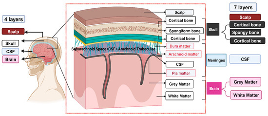
Figure 1.
The red dotted part shows the detailed human head tissue layers. Among all the layers, dura mater, arachnoid mater, and pia mater were not considered while making the sample. For the 4-layer head tissue model, the brain, CSF, skull, and scalp layers were considered. In the 7-layer head tissue model, white matter, grey matter, meninges, cortical bone, spongiform bone, cortical bone, and scalp layers were considered. The meninges in our 7-layered head tissue model are only represented by CSF.
For the purpose of EEG analysis, electrical conductivities are the most important parameters in accurate source localization and construction [7]. It is also important for the accurate understanding of the electrical activity in the live and postmortem brain tissues using EEG and MEG [8], which is critical to understanding the accurate neurological functions [9], neurological and psychiatric disorders [10], probable treatment [11], and recovery observations [12,13]. As such, the focus here is developing simulant materials with matching conductivities of head tissue materials. This is because any variation in Electrical conductivity in simulated human head layers has a huge impact on EEG source localization methods. In dipole reconstruction analysis, the conductivity of the skull and skin can impact the source localization up to 3 cm [14,15]. The human brain conductivity of both the white matter and grey matter layers has less impact on source localization but it can impact the strength and orientation of the sources [11].
Obtaining a skull from a cadaver is often difficult, and the experimental setup is complex and limiting. For this, many studies have been conducted to mimic the electrical properties of human head tissue layers. In [5,16], an effective single-layer head tissue model has been used. As different conductivity layers of head tissue can have different loss factors, such single-layer head tissue models may be inadequate for understanding layer-by-layer signal conduction and loss. In [2,4], a post-mortem human head skull with no scalp was used to study the EEG and MEG signal analysis. As the skull is one of the main barriers to ensure effective signal conduction, the role of the scalp and its conductivity cannot be ignored [14,15]. In [2,3], three layers of the human head model (brain–skull–‘pseudo’ scalp) were used for testing EEG equipment and source localization techniques. The CSF layer between the brain and skull has a significant effect [17] on the EEG sensitivity measurement. It can be understood that EEG sensitivity measurement studies may be prone to errors even if three layers are used in the phantom heads. Also, in the EEG source localization calculations, the distribution of spongiform bone thickness can affect the field potential on the scalp [18]. So, any design without detailed skull bone layers might affect EEG source localization calculations. In [19], a detailed human phantom head geometry was built using agar, gelatin, agarose, etc. In the study of [19], the material processing is simpler, but the final product did not provide the skull conductivity as it is harder to reach the skull conductivity using these materials [20]. In other studies [21,22], detailed phantom head geometry as well as the head tissue layer were built but most of the materials used were not durable and involved multiple components to create targeted geometry.
To design different layers of head tissue with matching electrical properties, it is first important to understand the electrical properties of brain layers and possible mechanisms of achieving the properties using phantom materials. Based on the most recent and comprehensive study on head tissue conductivities, it is known that the conductivity of each layer varies greatly [23]. Also, as the signal generated by the human brain is an analog signal, it changes with frequency [21,24]. Depending on the different mental tasks, the dominant frequencies and amplitudes of the sources vary. Therefore, the layers that have been manufactured for this study were tested in the targeted frequency range for conductivity. The validation of the targeted frequency range is explained in the results section in detail. There is also evidence of geometrical variations in human head sizes and the thickness of each layer of head tissues. Considering all the variations, it is not feasible to test each of them separately. Therefore, the goal within the specified frequency range is to build each layer that closely matches the suggested or median conductivities [23]. Reference [23] provides the range of conductivities of brain tissue layers based on many reported studies. A great focus is put on building a three-layer skull as the skull has the most effect on effective signal conduction [14,15]. The other head layers considered here are the ones that impose the greatest effect on EEG analysis [15,25]. Various researchers use different methods to construct different layers. The existing phantom materials serve two distinct purposes—one to match the mechanical properties [26,27] and the other to match the electrical properties. Oftentimes, many of the electrically equivalent phantom head materials are not durable, which severely limits its applications. Here, we use Composite materials for constructing different phantom layers. As the composite matrix is made using polymer, the durability is high [28]. In this method, conductive short fibers are mixed with nonconductive matrix material. The weight fraction of the conductive fibers is varied to tune the overall conductivity of the composites.
In this paper, multilayer head tissue is built using fiber-reinforced polymer Composite materials. Two types of models, namely a four-layer and a seven-layer head tissue model, have been designed, fabricated, and tested. The details of the fabrication procedure and our approach to tuning the electrical properties are discussed in the next section. The electrical properties of each layer are measured under different frequencies and compared with the corresponding head tissue materials. Finally, the effectiveness of the phantom layers is tested with an EEG and the results are discussed.
2. Materials and Method
The electrically equivalent phantom head materials were created using silicon composites. Different filler materials of different concentrations were tested to achieve the targeted conductivity. To produce a multilayer head phantom model, Polydimethylsiloxane (PDMS)–carbon fiber (PDMS-CF) composites are chosen. There are two steps involved in the making of a phantom head material with the desired Electrical conductivity. First, different filler materials of varying concentrations are selected to achieve the targeted conductivity. The test samples are made according to the specifications, as shown in Figure 2. Here, ‘Dielectric Spectroscopy’ has been used to study the conductivity of the composites at different frequencies. In the next step, the layers with the closest matching conductivity of human head layers are combined to construct the multilayer head phantom materials. In our study, since EEGs work on lower frequencies [3], the electrical permittivity of the material is not considered.
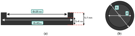
Figure 2.
The detailed dimensions of the single-layer sample for conductivity testing; (a) front view shows the inner (di) and outer (d0) diameter differences and thickness differences of extended lips and the main sample. (b) The top view provides the overall sample outlook. The samples were made in a circular shape to match the top copper plate shape of the conductivity measuring machine. All the dimensions are also according to the requirements and limitations of the conductivity measuring machine. Only the inner portion (di) was measured while measuring conductivity. The outer diameter (d0) and the thickness tl were built to hold liquid CSF while making a 4-layer sample.
We argue that the human head tissue can be divided into seven layers as shown in Figure 2 considering the scalp as one layer and ignoring subdural space [29]. In view of this, we have constructed two types of multilayer phantoms, namely the ‘Basic four layers’ (brain–cerebrospinal fluid (CSF)–skull–scalp) and the ‘Detailed seven layers’ types, as shown in Figure 1. Each layer has different material properties. The details of the head layers are shown in Table 1. After the confirmation of the conductivity testing, the 7-layered sample was tested for the capability of AC signal conduction using an EEG. As the 7-layered sample has the most possibility of signal loss, this sample has been chosen for EEG testing. The 7-layered sample was tested by wet EEG to confirm the validation of the sample while developing EEG systems.

Table 1.
Details of the as-fabricated head layers.
3. Experimental Procedure
3.1. Sample Preparation
The composites were all mixed in a weight-to-weight ratio. The matrix was PDMS, and the filler was carbon fiber (CF). The PDMS itself is an insulator material. The CF is a conductive filler. The concentration of carbon fiber affects the conductivity of the composite. The length of CF was kept at 1000 m and the width was 40 m. The CF was chopped using a commercially available stainless steel grinder at 1200 RPM. Each batch of chopped carbon fiber was then measured using a microscope to ensure the length of the fiber. The PDMS and carbon fiber were mixed at room temperature using a commercial resin mixer at 120 RPM for 30 min. Then, the hardener was measured and poured into the mixer, and mixed for another 15 min. The samples were poured into a mold and the degassing chamber was used to clear all air pockets inside the samples. The mold for the sample was printed using a 3D polymer printer. Each mold filled with the mixture was kept for 36 h at room temperature to cure. For each wt%, a minimum of 5 samples were manufactured and tested.
The top copper plate of the sample holder in dielectric spectroscopy has a radius of 12.5 mm, and the bottom plate has a radius of around 20 mm. So, the sample was designed accordingly. The dielectric spectroscopy would measure only volumes of the sample. The extended lips of thickness and diameter were designed to hold the liquid CSF while manufacturing a 4-layer head tissue model sample, seen in Figure 3a. For the 4-layer sample, the CSF was made by combining NaCl and DI water of desired conductivity [30]. The CSF was then injected into the hollow space between the skull and the brain layer. To ensure water-tight sealing between the layers, a thick layer of sealant was used. The sealant was made with a PDMS and CF (5 wt%) composite. The sealant layer was also dried for a day before injecting the NaCl and DI water mixture.
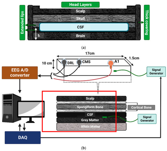
Figure 3.
(a) A 4-layer head tissue sample model. (b) This shows the EEG testing setup of a 7-layer sample. A 7-layer head tissue sample model is highlighted with the red line. The dimensions of these are mentioned in Table 1. For testing in the conductivity measuring machine, the signal generator was skipped from the layer. The signal generator was inserted in the grey matter area while processing the grey matter and CSF layer only for performing the EEG test. The signal generator tip was made of silver chloride and a signal was supplied from DAQ to the signal generator using copper wire. The dimensions of the sample shown here are for the EEG testing sample which was prepared according to the EEG electrode placing requirement.
For the 7-layer head tissue model’s multilayer samples, seen in Figure 3b, the sample diameter was kept at 40 mm and the thickness was varied for each layer.
It is observed that the typical skull thickness varies between men and women across different regions: frontal (men: 7.8 mm; women: 8.6 mm), parietal (men and women: 10.1 mm), occipital (men: 10.1 mm; women: 10 mm), and temporal (men and women: 6 mm) [31]. Additionally, the normal scalp thickness for adult humans is about 5.8 mm [32]. Cerebrospinal fluid (CSF) thickness ranges from 2.1 ± 0.9 mm to 6.3 ± 1.7 mm [33]. Gray matter (38 mm 12.7 mm) and white matter thickness (25.1 mm 11.3 mm) also vary, depending on the head surface location [34]. To maintain similar human head geometry, the minimum total thickness of a 7-layer model would be 77 mm. The maximum thickness for samples in dielectric spectroscopy is 11 mm. Variations in human head tissue thickness have an impact on the conductivity of specific layers. The variations in the thickness of human head tissues affect the conductivity of the specific layer [35,36]. Given the available resources, greater emphasis has been placed on matching electrical conductivity than on matching geometric thickness, as conductivity is the most important property that affects EEG research the most [7]. The thickness of each layer of the prepared sample is shown in Table 1. For each multilayer sample, the bottom layer has been prepared first. After curing the bottom layer, the next layer according to Figure 1 has been prepared and cured. Each layer has been measured using a digital screw gauge after curing. While pouring the sample solution into the mold, a measuring scale was used to determine the approximate thickness of each sample to ensure a consistent thickness. For multilayer samples, the newly produced layer thickness was obtained by subtracting the preceding layer’s thickness from the overall thickness of the measured layers. The CSF layer was made with a PDMS and CF composite. The liquid CSF was not used to make this layer. The reason behind this is the limitation of the dimensions of the dielectric spectroscopy machine’s sample holder. The thickness of each sample is limited to 11 mm. As there are more layers involved, the thickness of the sample was crossing the limitation of the thickness of the machine. To solve the problem, the CSF layer was made with a PDMS and Cf composite. For cortical bone layers, the mixture was poured into the mold, creating a thin layer. As the composite mixture viscosity was high, a paintbrush was used to spread the sample layer around the corner of the mold. Each of the layers was produced individually and cured for 24–36 h depending on the thickness of the layer. Thus, a batch of 7-layer tissue samples takes around 9 days to complete and a batch of 4-layer tissue samples takes 6 days to complete.
3.2. Conductivity Measurement Process
In a regular conductor, the valence band and conduction band overlap, creating a continuous band of energy states that allows charge carriers to move freely. On the other hand, PDMS (Polydimethylsiloxane) is nonconductive, displaying a disordered and amorphous structure, along with a substantial energy band gap [37] which causes the charge carriers to become confined within localized states, giving rise to a phenomenon known as hopping conductance. As a result, charge carriers can only migrate to neighboring empty states by jumping over a potential barrier and using quantum mechanical tunneling [38]. In this study, the conductivity of the PDMS sample was measured using Broadband Dielectric Spectroscopy (BbDS) (Novocontrol Technologies GmbH & Co. KG (Montabaur, Germany)). This technique has been widely employed in the polymer industry to analyze the electrical properties of polymeric materials. The experimental setup, illustrated in Figure 4, involves placing the sample material between two conductive electrodes. The diameter of the electrodes was maintained at 20 mm. A sinusoidal voltage (1 Vrms) is applied to one electrode, while the output current is measured through the other electrode. Depending on the material’s characteristics, the output current can either be in phase or out of phase with the input voltage signal. The conductivity of the material was measured over a frequency range of 1 Hz to 1 kHz at room temperature.
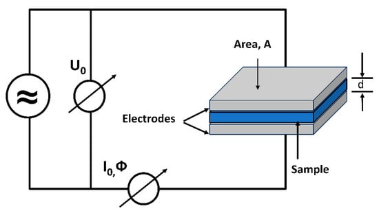
Figure 4.
The experimental setup for dielectric measurement of the sample.
To determine the complex conductivity, the first step is to measure the complex dielectric permittivity, ε*, as a function of frequency, ω. Once the complex permittivity data are obtained, mathematical relations between permittivity and conductivity are used to calculate the complex conductivity of the material. When a voltage U0(V) of fixed frequency (ω⁄2π) is applied to the sample, it results in a current I(A) at the same frequency, but with a phase shift (Φ).
These relations can be expressed in complex notation as shown below [39,40].
Here, U* = U0, I* = , and Re indicates the only real part of the complex notation. The magnitude of the current can be measured by the following equation:
Applying an electric field to a material leads to a phase shift between the current and voltage responses, and this phase angle can be measured by the following equation.
The impedance and capacitance of the sample can be determined using the equations provided below.
By utilizing the measured impedance and capacitance of the sample, the complex permittivity can be determined using the following equation:
and d is the gap between two electrodes.
Now, the second step requires Maxwell’s equation to calculate the complex conductivity. Complex conductivity includes both the real and imaginary (reactive) components. It considers both the steady-state flow of current and also takes into account the effects of capacitive and inductive components. In general, at very low frequencies, the real part of AC conductivity approaches DC conductivity. The complex conductivity can be expressed by [41,42]
Here, σ* is the complex conductivity, σ is the real part of the complex conductivity, i is the imaginary unit (√(−1)), ω is the angular frequency of the AC field (radians per second), and ε is the permittivity of the material. According to Maxwell’s equation, the current density (j) and the time derivative of the dielectric displacement () are equivalent.
By equating Equations (9) and (10), the expression for complex conductivity can be derived.
3.3. EEG Testing
The EEG testing was carried out to determine the validity of the prepared sample. The signal-to-noise (SNR) ratio was measured to validate the functionality of the layered sample while developing the EEG system. Since the prepared samples for measuring conductivity were small, a different dimension of sample Figure 3b was prepared to perform EEG testing. A signal generator probe was put inside the grey matter layer as electrical activity collected by the EEG is from this region [43]. The wet EEG has been used to collect the signal. As the sample was small, only one electrode was used. The EEG electrodes A1, CMS, and DRL were kept on the skin layer. A horizontal dipole has been created using a signal generator setup. Two ‘male to male’ wires placed horizontally in the grey matter layer with a positive and negative pole were generated using an in-house data acquisition system. The dipole signal generator was kept 10 cm away from the edge inside the grey matter layer. The EEG electrode A1 was also kept 10 cm away from the edge of the skin layer. The wet EEG uses electrolytic gel (Signa Gel, Parker Laboratories Inc., Fairfield, NJ, USA) over the human scalp to reduce signal loss. The skin layer was treated as real human skin and conductive gel was used on the top of the skin layer. All the EEG probes were connected with an analog to digital converter (A/D converter). The A/D converter was connected to the computer where data were measured and recorded. The signal generator was connected and controlled by the computer. The data acquisition system (DAQ) converted the command into signal generation. Although the real brain signal is a combination of different complex frequencies and amplitudes, here, a simple sine wave was supplied as a source. As the target is to test the feasibility of these layers for an EEG, the complex brain signal is not used. A simple sine wave of multiple frequencies and amplitudes was generated by the signal generator and recorded in a PC using Biosemi data acquisition software (ActiView 9.02). The recorded received signal is then used in MATLAB (R2021b) to calculate the SNR.
4. Results
4.1. Conductivity Test
The carbon fiber (CF) of approximately 1000 × 40 μm was chosen to make multilayer head tissue material. The filler material was chosen depending on the processibility and targeted conductive properties. Figure 5a shows the conductivity of different CF and PDMS concentrations. The frequency range was considered from 0 to 1000 Hz. Note that the neural activities in a clinically significant and normal human brain occur between 0 and 200 Hz [44,45]. We consider this as a low-frequency zone. High-frequency oscillation (HFO) can range up to 500 Hz in the epileptic region of a patient suffering from epilepsy [44,46,47].
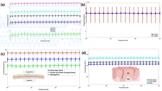
Figure 5.
(a) The effect of CF concentration on the conductivity of PDMS-CF composites. This study provides a functional relation between conductivity and CF concentration, which is then used to set the CF concentrations for different brain tissue layers based on their targeted conductivities. (b) Combined conductivity of 4-layer and 7-layer samples, which are nearly identical over the range of frequencies covered. Note that the 4-layered sample exhibits wider statistical variation than the 7-layered sample. (c) The conductivities of the whole skull and its sublayers (i.e., cortical and spongy layer) are shown. The inner and outer layer compact bones were made out of the same wt% composite. As the spongiform layer thickness is more than compact bones, the combined conductivity leans toward the spongiform bone’s conductivity. (d) The conductivities of brain tissue (combined white matter and grey matter), white matter, and grey matter are plotted.
In Figure 5a, we observe an increasing trend of conductivity with increasing CF concentrations. In addition, the conductivity of the composite within the targeted frequency zone is almost constant. From this study, we obtain a functional relation between CF concentration and the conductivity of the composites. Note that by varying the CF concentrations between 1% and 6%, the conductivities of the composite vary somewhere between 10−5 (S/cm) to 10−1 (S/cm). Table 2 shows the known electrical conductivities of different head tissue layers. It can be observed that the conductivities of head tissue layers vary between 10−5 (S/cm) to 10−2 (S/cm). As such, we can process different brain tissue layers with matching electrical conductivities by varying CF concentrations between 1% and 6%. The required carbon fiber concentration for each layer of head tissue is shown in Table 3. The corresponding electrical conductivities of head tissue layers are shown in Figure 5b–d. Figure 5b shows the conductivity of 4-layer and 7-layer head tissue samples. Figure 5c,d highlight the conductivity values of the skull and brain tissue layers. Note the variation in properties between the combined layers and their sublayers. Collectively, the measured conductivities provide various combinations of Electrical conductivity values of different regions of brain tissue as well as the whole tissue.
Table 2.
The conductivity lists of recommended, median values, and achieved conductivities of the head layers manufactured.
Table 3.
Carbon fiber concentration for each of the head layers manufactured.
The targeted conductivity values were chosen from the statistical study of human head tissue [23] as shown in Figure 6. Note that the values and the statistics reported in Figure 6 include 56 previously conducted experimental data points on various head tissue layers. The comparison between the achieved value and recommended value is also shown in Figure 6. The recommended value came from paper [23], where the study performed a statistical procedure called ‘meta-analysis’ for examining data from 56 independent studies and then determining average values. The median value has been taken from the boxplot diagram of the same study [23] which shows the variation in conductivity in different tissue layers. In Figure 6, the first and fourth solid line of each box is the first and third quartile accordingly. The third solid line of each box is the median of the study. Now, the recommended conductivity values [23] are available for a skull, its sublayers, CSF, brain tissue, white matter, gray matter, and scalp. In most cases, the recommended conductivity value of each layer or region is the median value obtained from the statistical analysis [23]. For further details on how the recommended values are obtained, the readers are referred to Ref. [23]. We set the composite composition for each layer to match the recommended values. From Figure 6 and Table 2, it can be observed that most of the achieved values are close to the recommended values. Although the spongiform’s targeted conductivity is much higher than recommended, the three-layer skull bone (outer compact–spongiform–inner compact) showed a similar conductivity compared to the recommended one. The brain layers (white matter and grey matter combined) do not have a recommendation in [23], but our combined GM-WM layer exhibits similar conductivity compared to the median value, as shown in Table 2. Table 2 also shows the specific values of the recommended and achieved conductivities of each layer. While not included in our current study, we also acquired the carbon fiber concentrations to align with the conductivities of the eye, cerebellum, spinal cord, and dura. It should also be noted that there are no data available on the combined conductivity of the whole head tissue. As our separate layers and sublayers match very well with the recommended values of the corresponding layers, we argue that the overall conductivity of the head tissue we report here reflects the overall conductivity of human head tissue, and the value can be used for models requiring conductivity of the whole head tissue.
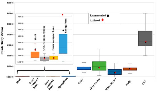
Figure 6.
Boxplot showing the variation in head tissue conductivity in different studies reported in [24]. It highlights the interquartile range, median, and extremes (minimum and maximum) of different head tissue layers that were manufactured. The recommended conductivity from study [23] is the black dot and the achieved conductivity [our study] from the sample for each layer is the red dot.
4.2. EEG and Signal-to-Noise (SNR) Ratio Calculation
The signal-to-noise ratio measures the ratio of the supplied signal and the noises received by the electrodes along with the supplied signal. The higher the signal-to-noise ratio, the more the electrodes receive the noise-free signal. The signal-to-noise ratio was the difference between the peak-to-peak amplitude between the source and the scalp potential. Here, the scalp potential refers to the data that were received by the EEG electrode. For practical purposes, noise can be added depending on the experimental requirement. Two types of SNR experiments were performed. In type A (), the amplitude of an artificially supplied sine wave was kept constant at 10 mV and the frequency varied from 10 to 1000 Hz. In type B (, the frequency of the sine wave was maintained at 10 Hz and the amplitude was varied. The amplitude of signals received by scalp or wet EEG is around 100 V [48]. However, the generated signal is supposed to be higher than the signal received by the scalp EEG. Electrocorticography (ECoG) which is referred to as subdural EEG places the electrodes directly on the surface of the brain [48]. As we placed our signal generator on the grey matter of the brain, the amplitude generated by the generator should be equivalent to the signal received by the ECoG. The signal amplitude SNR comparison between the EEG and ECoG [49] shows that ECoG has a 20–100 times higher SNR than the EEG. So, the amplitude range considered for the experiment was 500–20,000 or 0.5–20 mV.
In Figure 7a, the results of SNR for type are shown. There is a trend of increasing SNR between 0 and 100 Hz and 500 and 1000 Hz. The SNR drops between 100 and 500 Hz. All the SNR ratios except for 500 Hz show a positive value. This means that the signal received by the electrode is higher than the noise it received along with the signal. The highest SNR of 7.2616 dB for the experiments was found for 100 Hz. The lowest SNR of −1.71 dB was found for 500 Hz. In Figure 7b, the results for type are shown. A general increase in SNR with an increase in amplitude is observed with the exception of 10 mV. The SNR for the 10 mV amplitude still provides a positive SNR, which proves that the signal received is higher than the noise received with the signal. The lowest SNR of −9.9 dB is for the 0.1 mV amplitude, which is a very low amplitude. For this type of low-amplitude signal, different techniques can be applied to improve the SNR of received EEG signals [50].
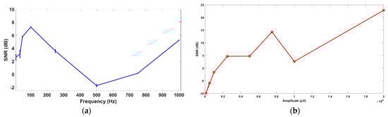
Figure 7.
(a) SNR for 1 mV amplitude and varying frequencies. (b) SNR for 10 Hz frequency and varying amplitude.
5. Discussion
In this study, we developed a multilayer electrically equivalent head tissue phantom and showed that the conductivities of individual layers as well as the overall conductivity of the four-layer and seven-layer head tissue are well within the reported values. The target conductivities of different layers of our human head tissue phantom were based on the report that summarized the conductivities of head tissue layers out of 56 independent studies [23]. We have shown that our Composite material system reasonably matches the desired conductivities, as shown in Figure 6. We argue that both our four-layer and seven-layer phantom models represent electrically equivalent phantom head tissue (Figure 1). As such, for future studies, any of these models can be used. However, our main motivation for building two different phantom tissues emanated from a specific application point of view. For instance, depending on the posture type of the human body (i.e., standing, sitting, or lying flat in a prone or supine position), the CSF layer thickness may vary, which, in turn, can alter the effective conductivity and signal intensity detected by an EEG [51]. In studies where CSF thickness variation matters the most, the four-layer model will be more suitable. When studies involve the effect of multiple factors such as CSF, skull, scalp, and depth of white matter or gray matter, then the seven-layer model should be used. The seven-layer model is also suitable for EEG studies where a more comprehensive phantom head tissue model is used. Such phantom head cases include skull, scalp, CSF, white matter, gray matter, eye, cerebellum [52], spinal cord, and dura [53]. By supplying any prerecorded data to the signal generator, the same response can be created in phantom heads, manufactured using any of these layers. Using these phantom heads, EEG equipment testing, electrode design upgrade and testing, as well as suitability testing of EEGs in various dynamic environments can be performed and compared especially when human subjects are not present.
Each of the layers individually and collectively can withstand the signal generation inside them without changing the electrical and physical properties of the material. Therefore, the SNR is unaffected by the signal supply inside the phantom layers over a lengthy period. When a phantom head is constructed utilizing these layers, several experiments can be carried out when conductivity is a major issue. As such, our modular material system is suitable for a wide range of applications. This study can offer a recipe for creating the layers as well as the ability to alter their thickness and geometry for any experiments examining the effect of only a single layer’s thickness on EEG errors [53,54]. The SNR study of the manufactured layers in Figure 7a,b can provide confidence in generating synthetic brain signals for the experiment [55,56].
It should be noted that all the studies only considered the electrical properties, mostly conductivity, but other properties like mechanical or thermal properties are not considered. For future work, head tissue layers capable of withstanding very high-frequency oscillation (VHFO) over 1000 Hz frequency [57] can be impactful in studying epileptogenic zones. The signal-to-noise ratio (SNR) for certain lower amplitude signals often exhibits negative values, indicating that the EEG receives more noise than the real signal. Such issues can be improved by changing the experimental setup or by improving the quality of the EEG probe. A full phantom head with human head geometry is not built and analyzed in this paper. So, the geometry modeling error will be present in the analysis of source localization. Most of the EEG studies conducted for detecting neurodegenerative disease, alertness level, and fatigue detection are performed by analyzing frequencies, especially the frequency power. These frequencies are known as dominant frequencies and vary depending on different human tasks. These dominant frequencies are divided into ranges such as Alpha (7–12 Hz) [58], Beta (12–30 Hz) [59], Gamma (25–50 Hz) [60], etc. These ranges are selected considering the fact of human subject variations. Also, in some studies such as inverse problems, the detailed geometric accuracy is considered unnecessary [61]. The source localization studies are the most affected by this geometric modeling error. In real life, when individual head scanning is not possible for source localization studies, changing some experimental setups such as increasing the number of electrodes [62], incorporating close to accurate skull conductivity in the calculation [63], and using more accurate 3D-measured co-registered electrode positions [63] has been suggested. So, tests include analyzing frequency power in certain regions of the brain in static and dynamic environments that can be performed with phantoms built using these layers.
Author Contributions
Conceptualization, A.A.; Methodology, R.R.D. and A.A.; Formal analysis, R.R.D., M.M.R. and Y.S.; Investigation, R.R.D.; Resources, R.R. and A.A.; Data curation, M.M.R., T.K. and Y.S.; Writing—original draft, R.R.D.; Writing—review & editing, R.R. and A.A.; Supervision, A.A.; Project administration, A.A.; Funding acquisition, A.A. All authors have read and agreed to the published version of the manuscript.
Funding
This work has been funded by the Force Health Protection (FHP) program through the Office of Naval Research (ONR) (Award # ONR: N00014-21-1-2051, ONR N00014-19-1-2383, and ONR N00014-20-1-2814: Timothy Bentley, Program Manager).
Data Availability Statement
The raw data supporting the conclusions of this article will be made available by the authors on request.
Conflicts of Interest
The authors declare no conflict of interest.
References
- Lopes da Silva, F. EEG and MEG: Relevance to Neuroscience. Neuron 2013, 80, 1112–1128. [Google Scholar] [CrossRef] [PubMed]
- Baillet, S.; Rira, J.J.; Main, G.; Magin, J.F.; Aubert, J.; Ganero, L. Evaluation of Inverse Methods and Head Models for EEG Source Localization Using a Human Skull Phantom. Phys. Med. Biol. 2001, 46, 77–96. [Google Scholar] [CrossRef] [PubMed]
- Collier, T.J.; Kynor, D.B.; Bieszczad, J.; Audette, W.E.; Kobylarz, E.J.; Diamond, S.G. Creation of a Human Head Phantom for Testing of Electroencephalography Equipment and Techniques. IEEE Trans. Biomed. Eng. 2012, 59, 2628–2634. [Google Scholar] [CrossRef] [PubMed]
- Leahy, R.M.; Mosher, J.C.; Spencer, M.E.; Huang, M.X.; Lewine, J.D. A Study of Dipole Localization Accuracy for MEG and EEG Using a Human Skull Phantom. Neuroimage 1998, 7, 159–173. [Google Scholar] [CrossRef]
- Peterson, S.M.; Ferris, D.P. Combined Head Phantom and Neural Mass Model Validation of Effective Connectivity Measures. J. Neural Eng. 2019, 16, 026010. [Google Scholar] [CrossRef] [PubMed]
- Omar, H.; Ahmad, A.L.; Hayashi, N.; Idris, Z.; Abdullah, J.M. Magnetoencephalography Phantom Comparison and Validation: Hospital Universiti Sains Malaysia (HUSM) Requisite. Malays. J. Med. Sci. 2015, 22, 19–27. [Google Scholar]
- Akhtari, M.; Bryant, H.C.; Emin, D.; Merrifield, W.; Mamelak, A.N.; Flynn, E.R.; Shih, J.J.; Mandelkern, M.; Matlachov, A.; Ranken, D.M.; et al. A Model for Frequency Dependence of Conductivities of the Live Human Skull. Brain Topogr. 2003, 16, 39–55. [Google Scholar] [CrossRef] [PubMed]
- Wendel, K.; Ieee, J.M. Correlation between Live and Post Mortem Skull Conductivity Measurements. In Proceedings of the 2006 International Conference of the IEEE Engineering in Medicine and Biology Society, New York, NY, USA, 30 August–3 September 2006; pp. 4285–4288. [Google Scholar] [CrossRef]
- Feyissa, A.M.; Tatum, W.O. Adult EEG. Handb. Clin. Neurol. 2019, 160, 103–124. [Google Scholar] [CrossRef]
- Cavanagh, J.F.; Napolitano, A.; Wu, C.; Mueen, A. The Patient Repository for EEG Data c Computational Tools (PRED + CT). Front. Neuroinform. 2017, 11, 67. [Google Scholar] [CrossRef]
- Smith, S.J.M. EEG in the Diagnosis, Classification, and Management of Patients with Epilepsy. Neurol. Pract. 2005, 76, ii2–ii7. [Google Scholar] [CrossRef]
- Barr, W.B.; Prichep, L.S.; Chabot, R.; Powell, M.R.; Mccrea, M. Measuring Brain Electrical Activity to Track Recovery from Sport-Related Concussion. Brain Inj. 2012, 26, 58–66. [Google Scholar] [CrossRef] [PubMed]
- Pournajaf, S.; Morone, G.; Straudi, S.; Goffredo, M.; Leo, M.R.; Salvatore, R.; Felzani, G.; Paolucci, S.; Filoni, S.; Santamato, A. Brain Sciences Neurophysiological and Clinical Effects of Upper Limb Robot-Assisted Rehabilitation on Motor Recovery in Patients with Subacute Stroke: A Multicenter Randomized Controlled Trial Study Protocol. Brain Sci. 2023, 13, 700. [Google Scholar] [CrossRef] [PubMed]
- Akalin Acar, Z.; Acar, C.E.; Makeig, S. Simultaneous Head Tissue Conductivity and EEG Source Location Estimation. Neuroimage 2016, 124, 168–180. [Google Scholar] [CrossRef] [PubMed]
- Vorwerk, J.; Aydin, Ü.; Wolters, C.H.; Butson, C.R. Influence of Head Tissue Conductivity Uncertainties on EEG Dipole Reconstruction. Front. Neurosci. 2019, 13, 531. [Google Scholar] [CrossRef] [PubMed]
- Oliveira, A.S.; Schlink, B.R.; Hairston, W.D.; König, P.; Ferris, D.P. Induction and Separation of Motion Artifacts in EEG Data Using a Mobile Phantom Head Device. J. Neural Eng. 2016, 13, 036014. [Google Scholar] [CrossRef]
- Wendel, K.; Narra, N.G.; Hannula, M.; Kauppinen, P.; Malmivuo, J. The Influence of CSF on EEG Sensitivity Distributions of Multilayered Head Models. IEEE Trans. Biomed. Eng. 2008, 55, 1454–1456. [Google Scholar] [CrossRef] [PubMed]
- McCann, H.; Beltrachini, L. Impact of Skull Sutures, Spongiform Bone Distribution, and Aging Skull Conductivities on the EEG Forward and Inverse Problems. J. Neural Eng. 2022, 19, 016014. [Google Scholar] [CrossRef] [PubMed]
- Owda, A.Y.; Casson, A.J.; Owda, A.Y.; Casson, A.J. Electrical Properties, Accuracy, and Multi-Day Performance of Gelatine Phantoms for Electrophysiology. bioRxiv 2020. bioRxiv:2020.05.30.125070. [Google Scholar] [CrossRef]
- Kandadai, M.A.; Raymond, J.L.; Shaw, G.J. Comparison of Electrical Conductivities of Various Brain Phantom Gels: Developing a “Brain Gel Model”. Mater. Sci. Eng. C 2012, 32, 2664–2667. [Google Scholar] [CrossRef]
- Mobashsher, A.T.; Abbosh, A.M. Three-Dimensional Human Head Phantom with Realistic Electrical Properties and Anatomy. IEEE Antennas Wirel. Propag. Lett. 2014, 13, 1401–1404. [Google Scholar] [CrossRef]
- Tseghai, G.B.; Malengier, B.; Fante, K.A.; Van Langenhove, L. A Long-Lasting Textile-Based Anatomically Realistic Head Phantom for Validation of Eeg Electrodes. Sensors 2021, 21, 4658. [Google Scholar] [CrossRef] [PubMed]
- McCann, H.; Pisano, G.; Beltrachini, L. Variation in Reported Human Head Tissue Electrical Conductivity Values. Brain Topogr. 2019, 32, 825–858. [Google Scholar] [CrossRef]
- Tang, C.; You, F.; Cheng, G.; Gao, D.; Fu, F.; Dong, X. Modeling the Frequency Dependence of the Electrical Properties of the Live Human Skull. Physiol. Meas. 2009, 30, 1293–1301. [Google Scholar] [CrossRef] [PubMed]
- Montes-Restrepo, V.; Van Mierlo, P.; Strobbe, G.; Staelens, S.; Vandenberghe, S.; Hallez, H. Influence of Skull Modeling Approaches on EEG Source Localization. Brain Topogr. 2014, 27, 95–111. [Google Scholar] [CrossRef] [PubMed]
- Baker, A.J.A.; Galindo, E.J.; Angelos, J.D.; Salazar, D.K.; Sterritt, S.M.; Willis, A.M.; Tartis, M.S. Mechanical Characterization Data of Polyacrylamide Hydrogel Formulations and 3D Printed PLA for Application in Human Head Phantoms. Data Brief. 2023, 48, 109114. [Google Scholar] [CrossRef]
- Knutsen, A.K.; Vidhate, S.; McIlvain, G.; Luster, J.; Galindo, E.J.; Johnson, C.L.; Pham, D.L.; Butman, J.A.; Mejia-Alvarez, R.; Tartis, M.; et al. Characterization of material properties and deformation in the ANGUS phantom during mild head impacts using MRI. J. Mech. Behav. Biomed. Mater. 2023, 138, 105586. [Google Scholar] [CrossRef] [PubMed]
- Raji, M.; Zari, N.; Bouhfid, R.; El Kacem Qaiss, A. Durability of Composite Materials during Hydrothermal and Environmental Aging; Woodhead Publishing: Cambridge, UK, 2018; ISBN 9780081022900. [Google Scholar]
- Yan, W.; Pangestu, O.D. A Modified Human Head Model for the Study of Impact Head Injury. Comput. Methods Biomech. Biomed. Eng. 2011, 14, 1049–1057. [Google Scholar] [CrossRef]
- Kamcev, J.; Sujanani, R.; Jang, E.S.; Yan, N.; Moe, N.; Paul, D.R.; Freeman, B.D. Salt Concentration Dependence of Ionic Conductivity in Ion Exchange Membranes. J. Membr. Sci. 2018, 547, 123–133. [Google Scholar] [CrossRef]
- Calisan, M.; Talu, M.F.; Pimenov, D.Y.; Giasin, K. Skull Thickness Calculation Using Thermal Analysis and Finite Elements. Appl. Sci. 2021, 11, 10483. [Google Scholar] [CrossRef]
- Bukhari, I.; Al Mulhim, F.; Al Hoqail, R. Hyperlipidemia and Lipedematous Scalp. Ann. Saudi Med. 2004, 24, 484–485. [Google Scholar] [CrossRef]
- Haeussinger, F.B.; Heinzel, S.; Hahn, T.; Schecklmann, M.; Ehlis, A.C.; Fallgatter, A.J. Simulation of Near-Infrared Light Absorption Considering Individual Head and Prefrontal Cortex Anatomy: Implications for Optical Neuroimaging. PLoS ONE 2011, 6, e26377. [Google Scholar] [CrossRef]
- Wendel-Mitoraj, K.; Malmivuo, J.; PROFILE Jari Hyttinen, S.A. Measuring Tissue Thicknesses of the Human Head Using Centralized and Normalized Trajectories View Project Hybrid Imaging System View Project 33 Publications 171 Citations See Profile. Conscious. Meas. 2009, 29, 112–113. [Google Scholar]
- Ferree, T.C.; Eriksen, K.J.; Tucker, D.M. Regional Head Tissue Conductivity Estimation for Improved EEG Analysis. IEEE Trans. Biomed. Eng. 2000, 47, 1584–1592. [Google Scholar] [CrossRef]
- Law, S.K. Thickness and Resistivity Variations over the Upper Surface of the Human Skull. Brain Topogr. 1993, 6, 99–109. [Google Scholar] [CrossRef] [PubMed]
- Schmerl, N.M.; Khodakov, D.A.; Stapleton, A.J.; Ellis, A.V.; Andersson, G.G. Valence Band Structure of PDMS Surface and a Blend with MWCNTs: A UPS and MIES Study of an Insulating Polymer. Appl. Surf. Sci. 2015, 353, 693–699. [Google Scholar] [CrossRef]
- Psarras, G.C. Hopping Conductivity in Polymer Matrix-Metal Particles Composites. Compos. Part A Appl. Sci. Manuf. 2006, 37, 1545–1553. [Google Scholar] [CrossRef]
- Vadlamudi, V. Assessment of Material State in Composites Using Global Dielectric State Variable; The University of Texas at Arlington: Arlington, TX, USA, 2019. [Google Scholar]
- Rabby, M.M.; Das, P.P.; Rahman, M.; Vadlamudi, V.; Raihan, R. Prepreg Age Monitoring and Qualitative Prediction of Mechanical Performance of Composite Using Dielectric State Variables. Polym. Polym. Compos. 2022, 30, 09673911221145053. [Google Scholar] [CrossRef]
- Poplavko, Y. Broadband Dielectric Spectroscopy; American Chemical Society: Washington, DC, USA, 2021; ISBN 9783642628092. [Google Scholar]
- Dong, M.; Ren, M.; Wen, F.; Zhang, C.; Liu, J.; Sumereder, C.; Muhr, M. Explanation and Analysis of Oil-Paper Insulation Based on Frequency-Domain Dielectric Spectroscopy. IEEE Trans. Dielectr. Electr. Insul. 2015, 22, 2684–2693. [Google Scholar] [CrossRef]
- Hinrichs, H. Electroencephalography; American Epilepsy Society: Chicago, IL, USA, 2013; ISBN 9781439860618. [Google Scholar]
- Bragin, A.; Engel, J.; Wilson, C.L.; Fried, I.; Mathern, G.W. Hippocampal and Entorhinal Cortex High-Frequency Oscillations (100–500 Hz) in Human Epileptic Brain and in Kainic Acid-Treated Rats with Chronic Seizures. Epilepsia 1999, 40, 127–137. [Google Scholar] [CrossRef]
- Velmurugan, J.; Sinha, S.; Satishchandra, P. Magnetoencephalography Recording and Analysis. Ann. Indian. Acad. Neurol. 2014, 17, S113–S119. [Google Scholar] [CrossRef]
- Frauscher, B.; von Ellenrieder, N.; Zelmann, R.; Rogers, C.; Nguyen, D.K.; Kahane, P.; Dubeau, F.; Gotman, J. High-Frequency Oscillations in the Normal Human Brain. Ann. Neurol. 2018, 84, 374–385. [Google Scholar] [CrossRef] [PubMed]
- Gotman, J. High Frequency Oscillations: The New EEG Frontier. Epilepsy Behav. 2013, 28, 309–310. [Google Scholar] [CrossRef][Green Version]
- Reilly, R.B.; Lee, T.C. Electrograms (ECG, EEG, EMG, EOG). Technol. Health Care 2010, 18, 443–458. [Google Scholar] [CrossRef] [PubMed]
- Ball, T.; Kern, M.; Mutschler, I.; Aertsen, A.; Schulze-Bonhage, A. Signal Quality of Simultaneously Recorded Invasive and Non-Invasive EEG. Neuroimage 2009, 46, 708–716. [Google Scholar] [CrossRef] [PubMed]
- Väisänen, O.; Malmivuo, J. Improving the SNR of EEG Generated by Deep Sources with Weighted Multielectrode Leads. J. Physiol. Paris. 2009, 103, 306–314. [Google Scholar] [CrossRef] [PubMed]
- Rice, J.K.; Rorden, C.; Little, J.S.; Parra, L.C. Subject Position Affects EEG Magnitudes. Neuroimage 2013, 64, 476–484. [Google Scholar] [CrossRef] [PubMed]
- Fernandez, L.; Rogasch, N.C.; Do, M.; Clark, G.; Major, B.P.; Teo, W.P.; Byrne, L.K.; Enticott, P.G. Cerebral Cortical Activity Following Non-Invasive Cerebellar Stimulation—A Systematic Review of Combined TMS and EEG Studies. Cerebellum 2020, 19, 309–335. [Google Scholar] [CrossRef]
- Ramon, C.; Garguilo, P.; Fridgeirsson, E.A.; Haueisen, J. Changes in Scalp Potentials and Spatial Smoothing Effects of Inclusion of Dura Layer in Human Head Models for EEG Simulations. Front. Neuroeng. 2014, 7, 32. [Google Scholar] [CrossRef]
- Hagemann, D.; Hewig, J.; Walter, C.; Naumann, E. Skull Thickness and Magnitude of EEG Alpha Activity. Clin. Neurophysiol. 2008, 119, 1271–1280. [Google Scholar] [CrossRef]
- Namazifard, S.; Daru, R.R.; Tighe, K.; Subbarao, K.; Adnan, A. Method for Identification of Multiple Low-Voltage Signal Sources Transmitted Through a Conductive Medium. IEEE Access 2022, 10, 124154–124166. [Google Scholar] [CrossRef]
- Namazifard, S.; Subbarao, K. Multiple Dipole Source Position and Orientation Estimation Using Non-Invasive EEG-like Signals. Sensors 2023, 23, 2855. [Google Scholar] [CrossRef] [PubMed]
- Usui, N.; Terada, K.; Baba, K.; Matsuda, K.; Nakamura, F.; Usui, K.; Tottori, T.; Umeoka, S.; Fujitani, S.; Mihara, T.; et al. Very High Frequency Oscillations (over 1000 Hz) in Human Epilepsy. Clin. Neurophysiol. 2010, 121, 1825–1831. [Google Scholar] [CrossRef] [PubMed]
- Mathewson, K.E.; Basak, C.; Maclin, E.L.; Low, K.A.; Boot, W.R.; Kramer, A.F.; Fabiani, M.; Gratton, G. Different Slopes for Different Folks: Alpha and Delta EEG Power Predict Subsequent Video Game Learning Rate and Improvements in Cognitive Control Tasks. Psychophysiology 2012, 49, 1558–1570. [Google Scholar] [CrossRef] [PubMed]
- Wang, D.; Miao, D.; Xie, C. Best Basis-Based Wavelet Packet Entropy Feature Extraction and Hierarchical EEG Classification for Epileptic Detection. Expert. Syst. Appl. 2011, 38, 14314–14320. [Google Scholar] [CrossRef]
- Coenen, F.; Scheepers, F.E.; Palmen, S.J.M.; de Jonge, M.V.; Oranje, B. Serious Games as Potential Therapies: A Validation Study of a Neurofeedback Game. Clin. EEG Neurosci. 2020, 51, 87–93. [Google Scholar] [CrossRef] [PubMed]
- Von Ellenrieder, N.; Muravchik, C.H.; Nehorai, A. Effects of Geometric Head Model Perturbations on the EEG Forward and Inverse Problems. IEEE Trans. Biomed. Eng. 2006, 53, 421–429. [Google Scholar] [CrossRef] [PubMed]
- Song, J.; Davey, C.; Poulsen, C.; Luu, P.; Turovets, S.; Anderson, E.; Li, K.; Tucker, D. EEG Source Localization: Sensor Density and Head Surface Coverage. J. Neurosci. Methods 2015, 256, 9–21. [Google Scholar] [CrossRef]
- Akalin Acar, Z.; Makeig, S. Effects of Forward Model Errors on EEG Source Localization. Brain Topogr. 2013, 26, 378–396. [Google Scholar] [CrossRef]
Disclaimer/Publisher’s Note: The statements, opinions and data contained in all publications are solely those of the individual author(s) and contributor(s) and not of MDPI and/or the editor(s). MDPI and/or the editor(s) disclaim responsibility for any injury to people or property resulting from any ideas, methods, instructions or products referred to in the content. |
© 2024 by the authors. Licensee MDPI, Basel, Switzerland. This article is an open access article distributed under the terms and conditions of the Creative Commons Attribution (CC BY) license (https://creativecommons.org/licenses/by/4.0/).