A Study on the Dynamic Response of a Timber-Frame Beam–Bamboo Anchor-Supported Roadbed Slope under Train Load

Abstract

In order to investigate the dynamic response of embankment slopes supported by wooden frame beams and bamboo anchor rods under train loading, this study conducted model tests on embankment slopes supported by wooden frame beams and bamboo anchor rods and carried out three-dimensional numerical simulations of the slopes. This study focused on analyzing the effects of train loading frequency, the peak value difference, and the peak value of the soil pressure on the embankment slopes. This study also analyzed the horizontal displacement of the slope surface, the internal forces in the support structure, and the slope safety factor. The results indicated the following: (1) The increase in loading frequency from 2 Hz to 3 Hz resulted in a significant increase in dynamic soil pressure, with a smaller increase observed upon further frequency increments. Moreover, increasing the load or peak value difference led to an overall increase in the maximum dynamic soil pressure. (2) Under various loading conditions, the axial force in the top anchor rod was significantly greater than that in the middle anchor rod. Additionally, the axial force in the rod body exhibited a pattern of larger forces near the anchorage end and smaller forces near the anchor head. The location of the maximum bending moment in the anchor rod transitioned from the anchor head to the anchorage end as the slope depth increased. The bending moment of the anchor rod increased with the loading frequency but decreased with an increase in the peak value, showing a minor influence from the upper and lower peak values. (3) With the presence of this support system, the slope safety factor increased by 20.13%. A noticeable reduction in the horizontal displacement of the slope surface was observed, with the greatest reduction in the top slope area, followed by the slope angle.

1. Introduction

The integration of environmentally friendly and ecologically sound support structures, which also ensure slope safety and reliability, has been a recent and current focal point of research among scholars. As a consequence of this, the emergence of “vegetation for slope protection” technology [1] has been garnering attention. Wu Hongwei [2] investigated the interactions among vegetation, the atmosphere, and soil. They discovered that vegetation not only reinforces the soil through its root system but also enhances soil suction through transpiration, thereby increasing soil shear strength and augmenting slope stability. Furthermore, Wang Yibing et al. [3] studied the hydraulic characteristics of reinforced clay slopes using vegetation combined with vegetation reinforcement strips. Their findings revealed that these reinforcement strips not only provided better reinforcement but also suppressed surface soil cracking. Der-Guey Lin et al. [4] established a three-dimensional numerical root model consisting of an inverted t-shaped rootstock and limiting hairy roots based on the actual root morphology in order to study the shear strength characteristics of the soil root system in Makino bamboo forests and successfully applied it to the numerical simulation of in situ uprooting tests of the soil root system.

This paper proposes a vegetation slope protection method that uses the combined support of live stumps and bamboo anchors [5,6]. Addressing the initial stage of live stump root development, a stage in which it fails to provide deep-root anchorage and shallow-root reinforcement to the slope [7,8], temporary support is applied to the roadbed slope using bamboo anchors and wooden frame beams. Previous studies have conducted experiments and three-dimensional numerical simulations on the use of wooden frame beam–bamboo anchor support systems under static loading conditions for slope protection. Yang H et al. [9] introduced an ecological slope-protection method—bamboo anchor wooden frame beams for initial support and indoor physical model experiments were conducted. Results indicated that under static loading, horizontal displacement initially occurred at the slope crest, but, ultimately, the horizontal displacement at the slope base exceeded that at the crest. Zhu Y et al. [10] performed indoor model experiments on four different forms of support using wooden frame beam–bamboo anchor systems for slope protection. The experiments demonstrated the significant effectiveness of the wooden frame beam–bamboo anchor support system, and optimizing the spacing between bamboo anchors and wooden frame beams enhanced its supportive effects. Jiang X et al. [11] conducted indoor model experiments applying static loads at the slope crest using the wooden frame beam–bamboo anchor support system. The study focused on the force characteristics of bamboo anchors and wooden frame beams and the slope surface displacement on cohesive soil slopes under this support.

Yan S. et al. [12] established a numerical model for roadbed slope under dynamic loading and verified its effectiveness through experiments. The results indicate that the maximum displacement of the roadbed slope increases with the amplitude of dynamic loading but decreases with an increase in load frequency. Ye S et al. [13] developed a dynamic response model for prestressed anchor beam-reinforced slopes, analyzing the dynamic soil pressure distribution, displacement of the frame-anchor structure, and the axial force distribution in the anchors. Gnanendran C. T. et al. [14] conducted small-scale physical model experiments to investigate the effect of dynamic loading frequency on the strip foundation at the crest of slopes. They found that cyclic loading can enhance the bearing capacity of the foundation soil. However, as the dynamic loading frequency increases, the increment in bearing capacity diminishes, leading to increased non-elastic deformations of the slope in both inclined and vertical directions. Qiu H. Z. et al. [15] used finite element software to study the dynamic response of excavation slopes under vehicle loading. They observed that, as the load position moves closer to the support structure, the displacement and deformation of the support structure increase, along with increased axial forces in the anchors. Additionally, with an increase in loading frequency, the deformation of the support structure increases, while the axial forces in the anchors decrease.

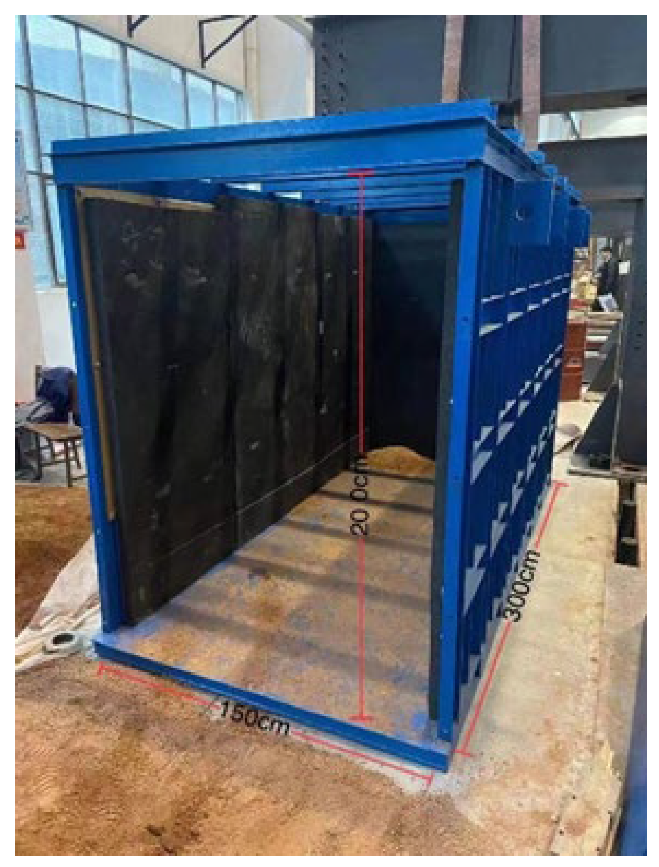
The majority of the aforementioned studies have focused on model experiments and three-dimensional numerical simulations of roadbed slopes under static loading. However, investigating the dynamic response of roadbed slopes under train loading holds significant research significance. This paper targets the support of roadbed slopes using bamboo anchors and wooden frame beams, employing a model experiment approach. It aims to explore the dynamic response of roadbed slopes supported by wooden frame beams and bamboo anchors under train loading. This research aims to provide a reference basis for studying the dynamic response of roadbed slopes under the combined support of live stumps and bamboo anchors.

2. Model Test Program

2.1. Model Box

The dimensions of the model box are 300 cm (net length) × 150 cm (net width) × 200 cm (net height). To mitigate boundary effects during hydraulic fatigue loading of the model box, thick high-density polyethylene black foam boards, approximately 5 cm in thickness, are adhered to the inner sides of the model box as energy-absorbing materials. The model box is illustrated in Figure 1.

2.2. Determination of Similarity Relations

According to dimensional analysis [16], the similarity ratio between the model box and the physical quantities related to the actual slope is controlled. Utilizing dimensional matrices and the principle of dimensional homogeneity, the similarity constants for various physical quantities are derived. The main physical quantities are shown in

Table 1. Similarity relationship.

Physical Quantities	Similarities	Similarity Constants
Geometric dimensions l	Cl	7
Elastic modulus E	CE	1
Density ρ	Cρ	1
Dynamic loading P	CP = (Cl)2Cρ	49
Internal friction angle φ	Cφ	1
Cohesion c	Cc = CE	1
Poisson ratio μ	Cμ	1
Dynamic displacements u	Cu = Cl	7
Stress σ	Cσ = CE	1
Time t	Ct = (Cl)(Cρ)1/2(CE)−1/2	7

.

2.3. Test Parameters

Prior to conducting indoor slope model experiments, relevant parameter tests were performed on the test materials. The optimum moisture content for red clay and sand-mixed red clay (at a ratio of 3:1) was found to be 13.5% and 12.5%, respectively, while their respective maximum dry densities were 1.87 g/cm³ and 1.97 g/cm³. Tensile tests were conducted on bamboo anchors and wooden frame beams to measure their elastic moduli and Poisson’s ratios. The main test parameters are presented in

Table 2. Test parameters.

Material Names	Model Types	Elastic Modulus (MPa)	Poisson Ratio	Capacity (kN/m3)	Cohesion (kN/m2)	Internal Friction Angle (°)
Bamboo Anchors	Elasticity	12,500	0.28	7.8	-	-
Wooden frame beam	Elasticity	14,300	0.36	9.6	-	-
Clay	Moorcullen	65	0.32	17.8	12	18.5
Clay (sand mixing)	Moorcullen	68	0.35	18.0	10	16

.

2.4. Strain Gauge Arrangement

As shown in Figure 2, the arrangement of strain gauges on the bamboo anchors is depicted. Prior to the slope test, strain gauges were placed at intervals of 10 cm, 22.5 cm, 35 cm, 47.5 cm, and 60 cm from the anchor head. The measurement points, numbered from 1 to 5, correspond sequentially from the thinner end (anchor head) to the thicker end (anchor tip). The total length of the bamboo anchor is 70 cm.

As shown in Figure 3, the arrangement of strain gauges on the wooden frame beam is illustrated. Seven strain gauges were affixed to each of the first row’s horizontal beams and middle vertical beams. For the horizontal beams, starting from the second span, strain gauges were applied at intervals of 12.5 cm, labeled from left to right as measurement points H1 to H7. For the vertical beams, starting from the first span, strain gauges were attached at intervals of 16.33 cm, labeled from top to bottom as measurement points S1 to S7.

2.5. Slope Physical Model

The experiment consisted of two sets, divided into the original unsupported slope and the slope reinforced with three rows of bamboo anchors and wooden frame beams. As illustrated in Figure 4, the soil in the experiment was divided into five layers from bottom to top. The bottom layer represented the foundation soil to simulate the base soil of the slope. The second layer comprised red clay typical of Hunan Province. The third layer represented the bottom layer of the subgrade, filled with a mixture of sand and red clay (in a 3:1 ratio). The fourth layer simulated the surface layer of the subgrade, also filled with the same mixture of sand and red clay. The fifth layer was the ballast layer, mainly consisting of crushed stones beneath the railway track. The slope ratio of the soil slope was 1:1, with the foundation layer being 20 cm high, the embankment layer 100 cm high, the bottom layer of the subgrade 27 cm high, the surface layer of the subgrade 9 cm high, and the slope ratio of the subgrade layer was 4%. The ballast layer was 6 cm high, with a slope ratio of 1:1.75. The total height of the slope was approximately 160 cm, with a length of around 250 cm and a width of about 140 cm. The average compactness of each layer, as measured in the experiment, met the requirements specified in the “Design Specifications for Heavy-duty Railways”.

The vertical soil pressure cells—labeled D, C, B, and A—were placed vertically downward from the loading point at the crest of the slope at distances of 15 cm, 40 cm, 65 cm, and 90 cm, respectively. Electronic displacement transducers denoted as C1 to C5 were installed parallel to the ground surface from the crest to the slope toe. The slope soil was compacted near its optimum moisture content, and, as indicated in Figure 5, electronic displacement transducers were mounted on the slope surface and connected to the Donghua data acquisition instrument. Strain gauges were attached to both the bamboo anchors and wooden frame beams, buried within the slope, and connected to the IMC data acquisition instrument. Different sinusoidal train loads were applied to the sleepers at the crest of the slope under varying working conditions, and relevant experimental data were collected during this process.

2.6. Loading Scheme Design

Taking into account various traffic load parameters [17,18], vehicle speed factors, and the effect of the vehicle’s load, the train load was considered to be a sinusoidal waveform for loading the railway embankment slope. The specific application process of load in the test process is through the hydraulic fatigue machine to simulate the train load in the form of cyclic load applied to the railroad sleeper, in the thick steel plate of the railroad sleeper pad, in the steel plate on the placement of the distribution beam, and in a hydraulic fatigue machine actuator, to apply the load to ensure the train load uniformity of the role of the rails on the sleeper. Considering model similarity ratios and the dynamic stress response of the train load, following the Railway Subgrade Design Code, the four 250 kN axle loads were converted into distributed loads and then scaled to the model. The peak value of the dynamic load was calculated as follows:

$$P_d=\frac{P_j}{d\times C_L}\times l\times \left(1.4+i\right)=\frac{250}{1.4\times 7}\times 0.6\times (1.4+0.5)=29.1 \mathrm{k}\mathrm{N}$$

The parameters are defined as follows: $P_d$ is the peak load applied to the model; $P_j$ is the static load; d is the spacing between axles; $C_L$ is the model similarity ratio; $l$ represents 0.6, the longitudinal length of the model track; 1.4 stands for the live load combination factor; and i represents the design impact coefficient set at 0.5. The specific experimental conditions for each scenario are presented in

Table 3. Loaded working condition table.

Work Conditions	Frequency (Hz)	Lower Peak (kN)	Peak Difference (kN)	Upper Peak (kN)
1	2	15	14.1	29.1
2	3	15	14.1	29.1
3	4	15	14.1	29.1
4	3	12.24	14.1	26.65
5	3	17.76	14.1	31.86
6	3	20.52	14.1	34.62
7	3	15	11.1	25.1
8	3	15	17.1	32.1
9	3	15	20.1	35.1

below.

3. Analysis of Slope Model Test Results

3.1. The Variation Law of Vertical Dynamic Ground Pressure

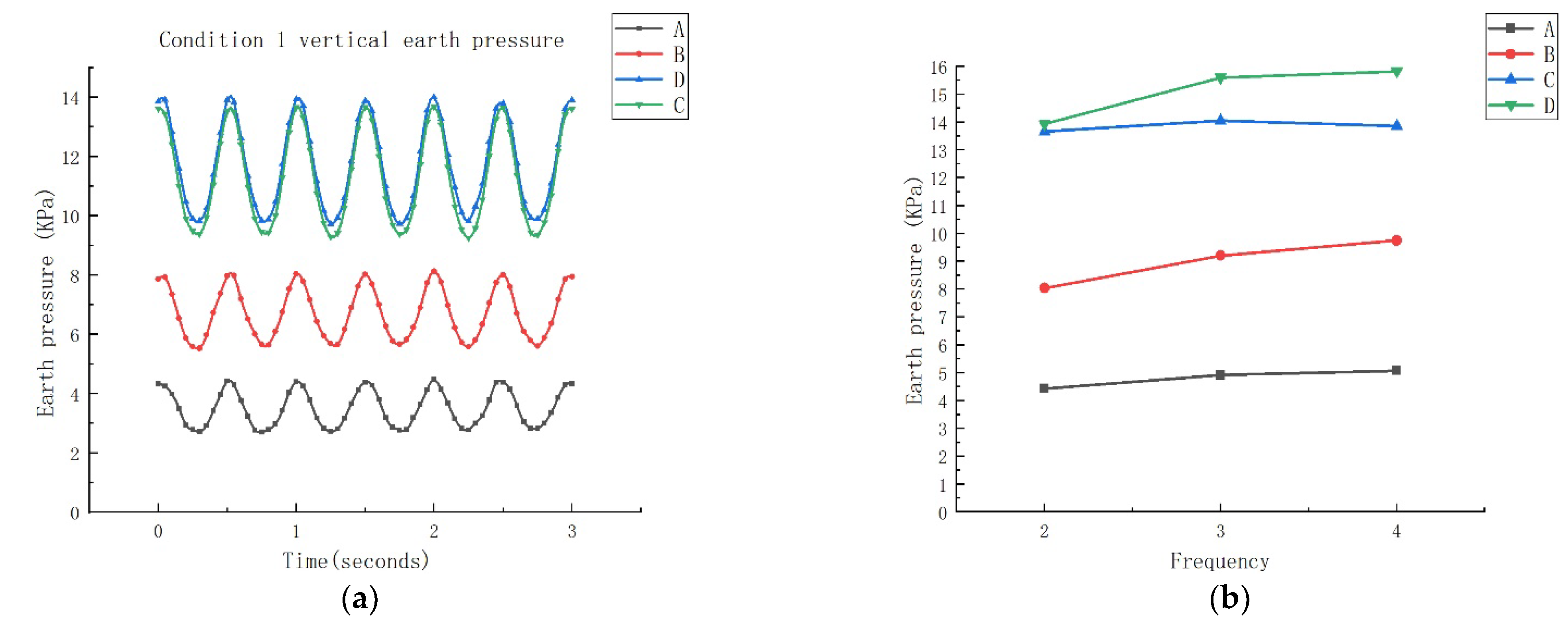
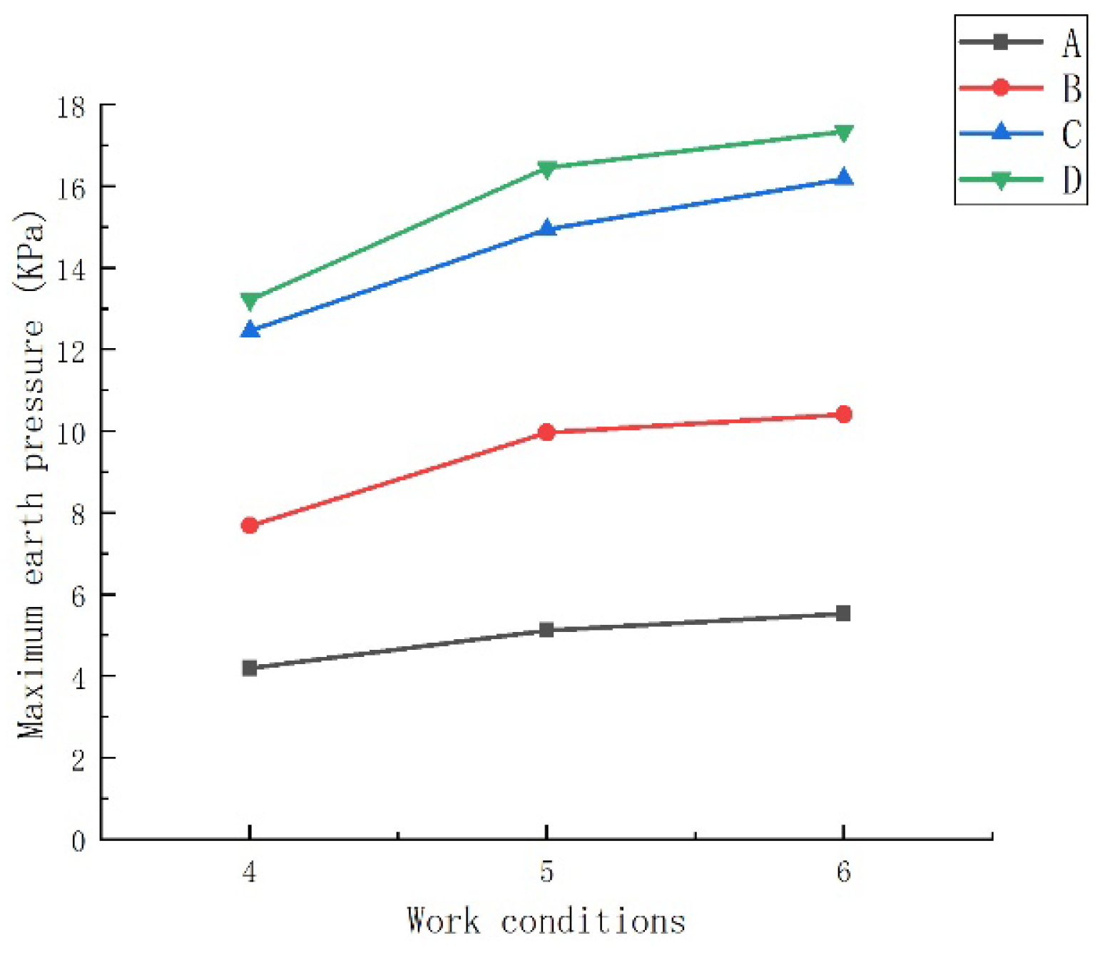
As depicted in Figure 6a,b, Figure 6a illustrates the vertical dynamic soil pressure curve at a loading frequency of 2 Hz, while Figure 6b displays the maximum dynamic soil pressure under various loading frequencies. When the loading frequency ranges between 2 and 4 Hz, the vertical dynamic soil pressure exhibits a similar sinusoidal pattern in correlation with the crest load. The dynamic soil pressure gradually decreases with increased burial depth, and as the burial depth increases, the peak values of the soil pressure curves become progressively closer to each other. At a loading frequency of 2 Hz, the maximum dynamic soil pressure at point D slightly surpasses that at point C. When the loading frequency is raised to 3 Hz, there is a noticeable increase in the maximum dynamic soil pressure at all measurement points. However, as the loading frequency continues to increase to 4 Hz, the rate of increase in the maximum soil pressure at each point slows down.

Figure 7 illustrates the maximum vertical dynamic soil pressure under various peak-to-peak loadings. With the increase in the peak-to-peak loading, the maximum dynamic soil pressure at points A to D initially experiences a sharp rise. Additionally, for shallower burial depths, the increment in pressure is more significant. Subsequently, while the maximum soil pressure at each point continues to increase with the rise in peak-to-peak loading, the rate of increase at each point diminishes.

Figure 8 displays the maximum vertical dynamic soil pressure under constant amplitude differential loading. With the increase in the upper peak value, the increments at points A to D are 1, 1.5, 2.5, and 3 kPa, respectively. The curves representing the maximum dynamic soil pressure at each measurement point consistently maintain the lower peak value while adhering to the observed pattern of increment in the upper peak value.

The vertical dynamic soil pressure curves exhibit a sinusoidal pattern similar to crest loading across all loading conditions. The maximum dynamic soil pressure at each measurement point increases with depth, indicating that in model experiments, stress diffusion may become more apparent as the slope depth increases. Additionally, a significant portion of the force might dissipate due to friction between the slope and the model box. Hence, in engineering practice, as the burial depth decreases, the accuracy of soil pressure calculations tends to improve. When the frequency increased from 2 Hz to 3 Hz, there was a substantial increase in soil pressure; however, with a further increase to 4 Hz, the increase in soil pressure was comparatively smaller. The increase in load also demonstrated a positive correlation with soil pressure, whether it was an increase in peak-to-peak values or peak value differentials, resulting in a continual increase in maximum dynamic soil pressure.

3.2. The Law of Change of Horizontal Displacement of Slope Surface

As shown in Figure 9, under the effect of crest loading at 2 Hz, the maximum horizontal displacement of the slope surface varied at different points. At points C1 and C2, the maximum horizontal displacement decreased. Particularly, at point C1, the reduction was at its most significant, decreasing from an outward protrusion of 1.3 mm to 0.1 mm, marking a reduction of nearly 92%. At point C3, the maximum horizontal displacement of the slope surface slightly increased, from a slight inward depression to 0.1 mm. However, at points C4 and C5, there was only a minimal change in the maximum horizontal displacement of the slope surface.

As depicted in Figure 10, under the effect of crest loading at 3 Hz, the maximum horizontal displacement of the slope surface exhibited varying trends at different measurement points. At points C1 and C2, the maximum horizontal displacement of the slope surface decreased. Specifically, at these points, the displacement reduced from the outward protrusion of 0.4 mm and 0.1 mm to 0.2 mm and 0.05 mm, respectively, marking a reduction of nearly 50% at both locations. Conversely, at points C3 and C4, the maximum horizontal displacement of the slope surface increased. At these points, the displacement shifted from an inward depression of 0.05 mm and 0.02 mm to 0.2 mm. However, at point C5, there was no significant change in the maximum horizontal displacement of the slope surface.

As shown in Figure 11, under the effect of crest loading at 4 Hz, the maximum horizontal displacement of the slope surface exhibited varying trends at different measurement points. At point C1, the maximum horizontal displacement of the slope surface decreased significantly from an outward protrusion of 1.3 mm to 0.25 mm. At point C2, the maximum horizontal displacement decreased from an outward protrusion of 0.35 mm to an inward depression of 0.15 mm. Conversely, at point C3, the maximum horizontal displacement increased from an inward depression of 0.05 mm to 0.15 mm. However, at points C4 and C5, there were no significant changes in the maximum horizontal displacement of the slope surface.

As shown in Figure 12, with the increase in the peak-to-peak crest loading, the maximum surface displacement at various measurement points demonstrated different trends. At point C1, the maximum surface displacement slightly increased and then remained relatively stable. At point C2, the maximum surface displacement decreased from an inward depression of 0.1 mm to 0 mm. Meanwhile, at point C3, the maximum surface displacement increased from 0.15 mm to 0.2 mm. At point C4, the maximum surface displacement slightly increased before stabilizing. Additionally, at point C5, the maximum surface displacement initially remained unchanged and then slightly increased to an outward protrusion of 0.15 mm.

As depicted in Figure 13, with the increase in the peak value differential of the crest loading, the maximum surface displacement at various measurement points showed distinct changes. At point C1, the maximum surface displacement decreased from an outward protrusion of 0.23 mm to 0.18 mm. At point C2, the maximum surface displacement increased from an inward depression of 0.2 mm to 0.7 mm. However, at points C3, C4, and C5, the maximum surface displacement remained relatively unchanged and maintained a consistent pattern.

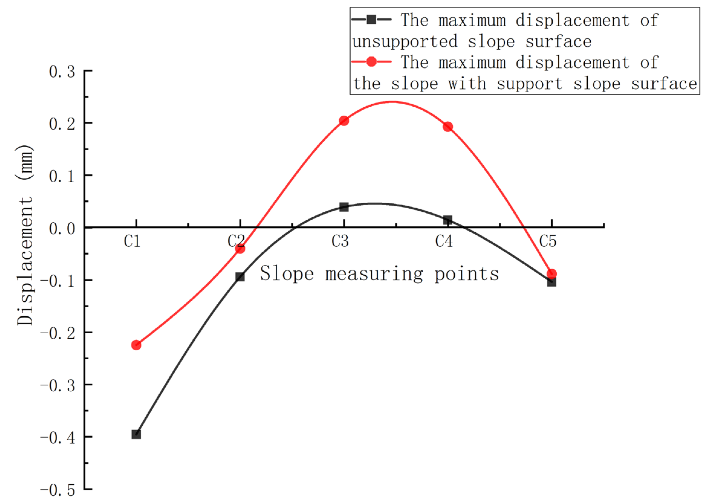
Under crest loading, the slope surface exhibits outward protrusion at the slope crest and slope toe regions, while it shows inward depression in the middle section of the slope. Compared to the unsupported slope, significant reductions in the maximum horizontal surface displacement are observed at various measurement points when the slope is supported. Point C1 at the crest experiences the most substantial decrease in the maximum surface displacement, followed by slightly smaller reductions at points C2 (crest) and C5 (toe), whereas points C3 and C4 in the middle section show no significant variation. This could be attributed to the proximity of point C1 to the loading area, leading to a more pronounced effect of the crest load. Therefore, in practical applications, particular attention should be given to reinforcing and monitoring the support at the crest and toe positions, emphasizing the comprehensive implementation of the wooden frame beam–bamboo anchor support. The considerable reduction in the maximum horizontal surface displacement on the slope surface with the wooden frame beam–bamboo anchor support demonstrates the feasibility of using this system as temporary support for railway embankment slopes.

3.3. Bamboo Anchor Shaft Force Variation Law

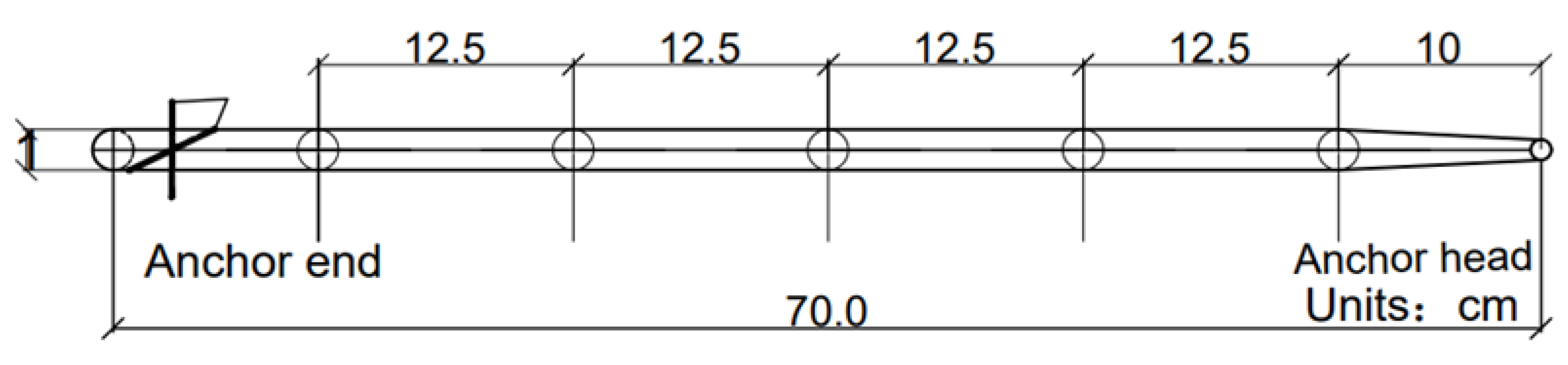
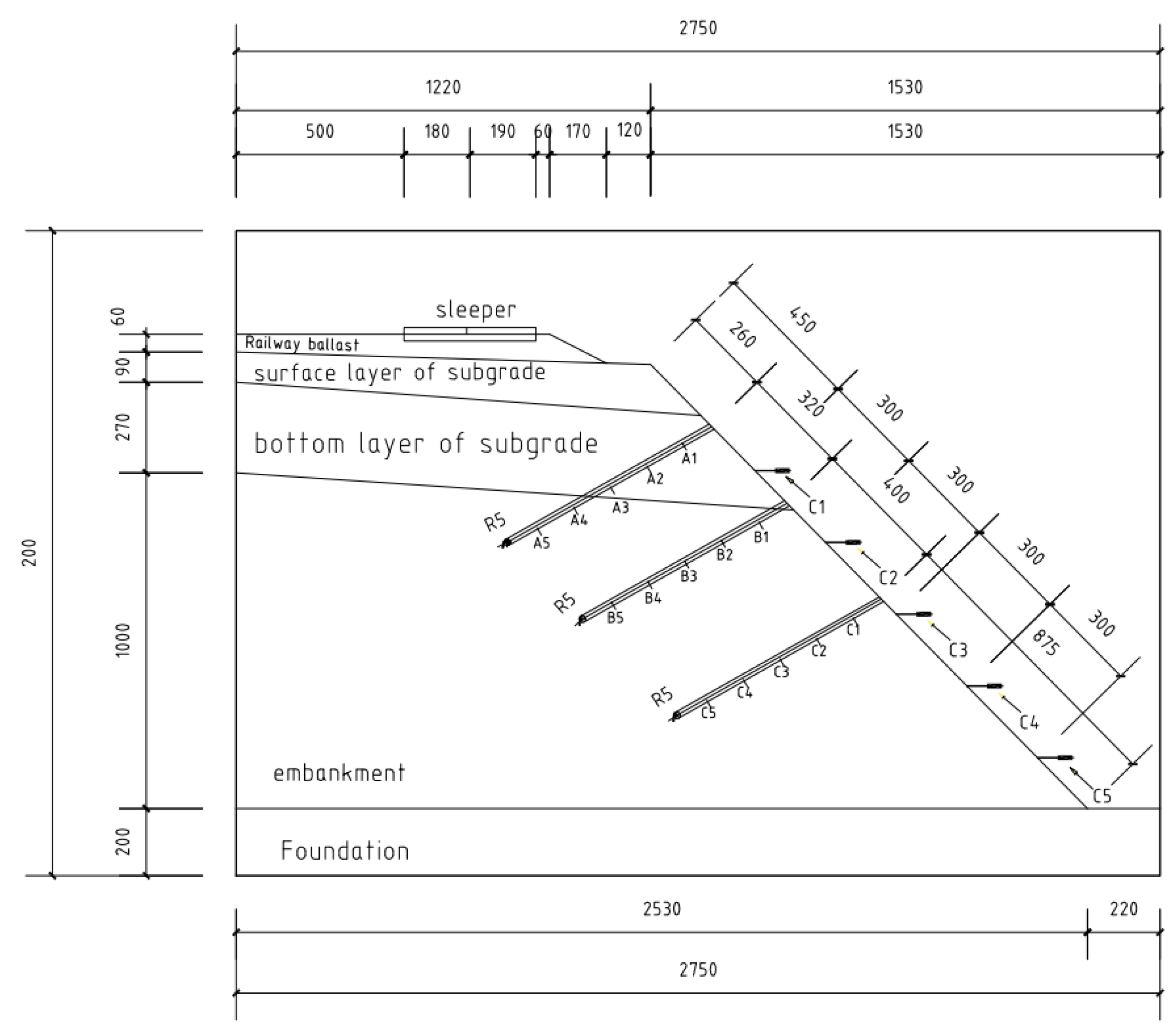
As shown in Figure 14, the bamboo anchor rods are installed at an angle of 105 degrees with respect to the slope surface. The anchoring end is embedded within the slope, while the anchor head is connected to the wooden frame beam, forming an integrated support system. According to Formula (1), the normal stress on the cross-sectional area of the bamboo anchor rod is represented, where the axial force of the bamboo anchor rod is the cross-sectional area, and is the modulus of elasticity of the bamboo anchor rod. By employing Formulas (1) and (2), the axial force of the bamboo anchor rod can be determined as shown in Equation (3).

$$\sigma =\frac{F_N}{S_0}$$

(1)

$$E=\frac{\sigma }{\epsilon }$$

(2)

$$F_N=E\epsilon S_0$$

(3)

$$\mathrm{Anchor} \mathrm{bending} \mathrm{moment}: M=EW{\epsilon }_M$$

(4)

where $W$ is the flexural section modulus of the bamboo anchor taken as $\frac{3\pi d}{16}$, and ${\epsilon }_M$ is $\frac{1}{2}$ of the measured strain due to the bending moment using the half-bridge wiring method.

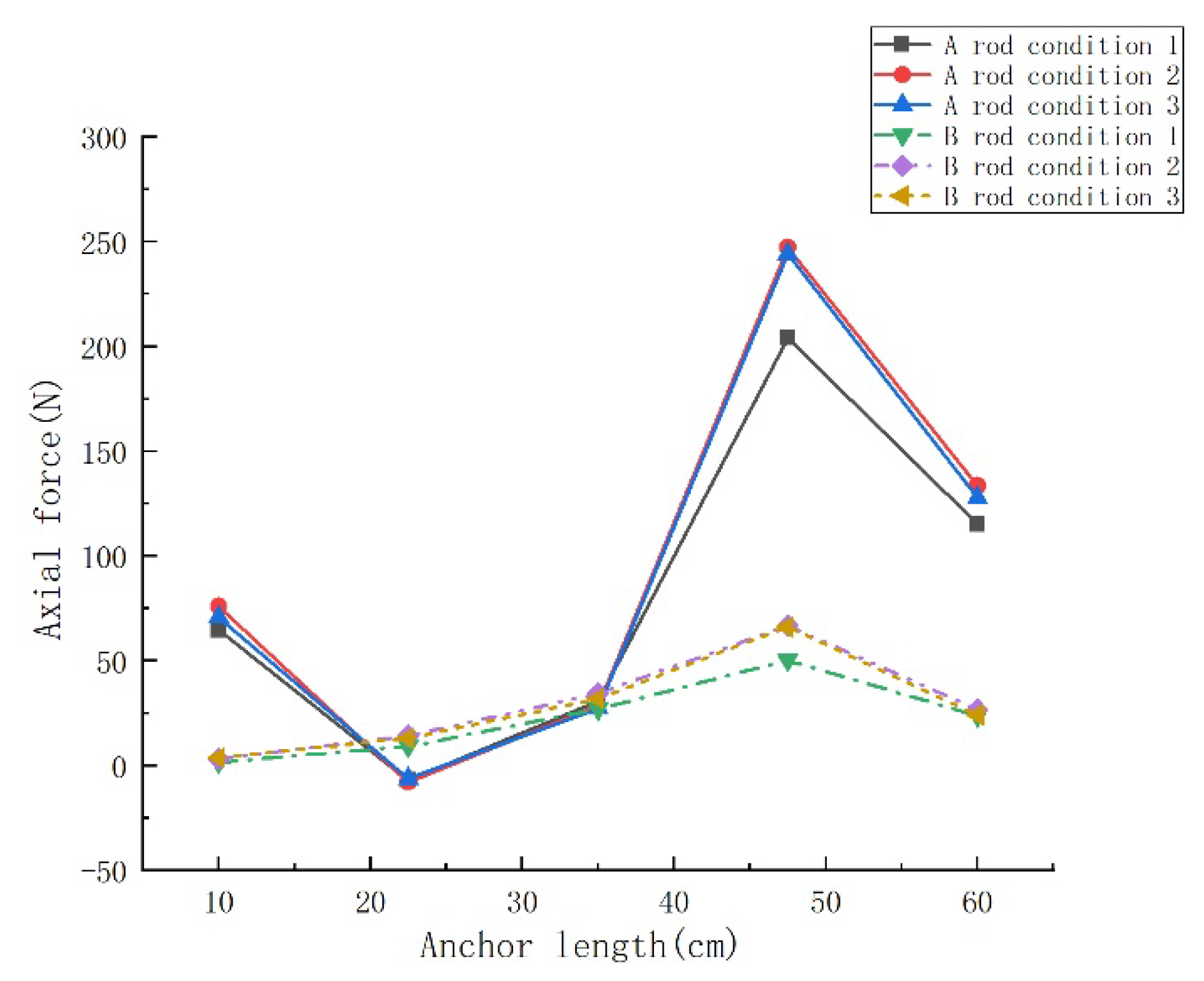
The axial forces at various measurement points for Rod A and Rod B under different loading frequencies are illustrated in Figure 15. For Rod A, except at point A2 where it experiences compression, the other measurement points endure tension. Among these points, A4 exhibits the maximum tensile force, while A3 shows the minimum tensile force across all conditions. When the frequency escalates to 3 Hz, apart from points A2 and A3, the axial forces at the remaining points increase to varying degrees. However, with the frequency further increased to 4 Hz, the axial forces in Rod A slightly diminished instead.

On the other hand, the overall axial force in Rod B is smaller than that in Rod A. Rod B experiences tension at all measurement points under loading, except for point B1, which transitions from tension to compression at 4 Hz loading. Throughout all conditions, B4 manifests the maximum tensile force among the measurement points for Rod B. As the loading frequency increases to 3 Hz, the axial forces at different points in Rod B increase to varying extents, with the most significant increment observed at point B4. However, when the loading frequency rises to 4 Hz, there is no noticeable change in the axial forces.

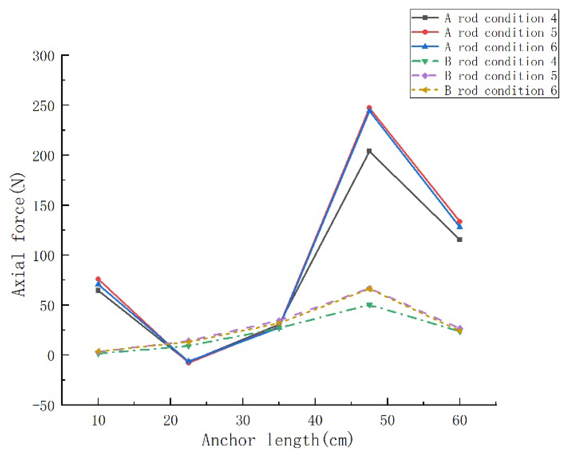
The axial forces at various measurement points for Rod A and Rod B under different peak-to-peak loading conditions are depicted in Figure 16. In all scenarios, except at point A2, all measurement points for Rod A experience tension, with A4 exhibiting the maximum tensile force. When the peak-to-peak loading increases to condition 5, the axial force at A4 noticeably increases; however, with further increments in the peak-to-peak loading, the axial force slightly decreases.

In comparison to Rod A, all measurement points for Rod B experience tension, with the axial force gradually increasing from the anchor head to the anchoring end until point B4, where it decreases. Notably, B4 exhibits the maximum tensile force. With the increase in the peak-to-peak loading, the axial forces in Rod B initially show a certain degree of augmentation, followed by a trend toward stabilization.

The axial forces at various measurement points for Rod A and Rod B under different peak differential loading conditions are illustrated in Figure 17. For Rod A, except at point A2, all measurement points experience tension. The maximum axial force for Rod A is consistently observed at A4 in all conditions. The distribution pattern of axial forces along the rod reveals a trend where the force gradually decreases from the anchor head towards the anchoring end, initially exhibiting compression and then transitioning to tension, reaching its peak at point A4. As the upper peak value increases to condition 8, the axial force in the rod shows no significant change; however, upon reaching condition 9, there is a sudden drop in the rod’s axial force.

In comparison to Rod A, all measurement points for Rod B experience tension, with the maximum axial force occurring at B4. The axial force distribution along the rod gradually increases from the anchor head towards the anchoring end, reaching its peak at position B4, and subsequently decreasing. Interestingly, in Rod B, as the upper peak value increases, the axial forces at all measurement points decrease.

In various conditions, the axial force in Rod A at the slope top is significantly larger than that in Rod B at the slope middle. The closer the rod is to the top of the slope, the greater the axial force distribution along the rod. This indicates that the effect of Rod A at the slope top on slope support is more pronounced. The axial forces in the anchor rods show a pattern of larger forces at the anchoring end and smaller forces at the anchor head. Therefore, it is deemed unreasonable in engineering practice to assume a uniform distribution of axial force along the length of the anchor rod.

Within the support system, Rod A, situated closer to the loading point near the slope top, takes the lead in providing support, transitioning subsequently to the anchor rods at the slope middle and slope angle. The maximum value of axial force in the rod appears at measurement point 4, closer to the anchoring end. This phenomenon is due to the anchoring end’s proximity to the potential slip surface of the slope, causing the axial force in the anchor rod to reach its maximum as a result of shear displacement along the potential slip surface.

The axial force in the anchor rod shows an initial positive correlation in increase, both in frequency and upper and lower peak values, followed by no significant increase in the later stage. However, when only the upper peak value increases, the axial force on the anchor rod decreases. This reduction may be attributed to the transition of axial force in the anchor rod as the upper peak value increases, gradually distributing the force across the entire support system, collectively resisting slope movement.

3.4. Bamboo Anchor Bending Moment Analysis

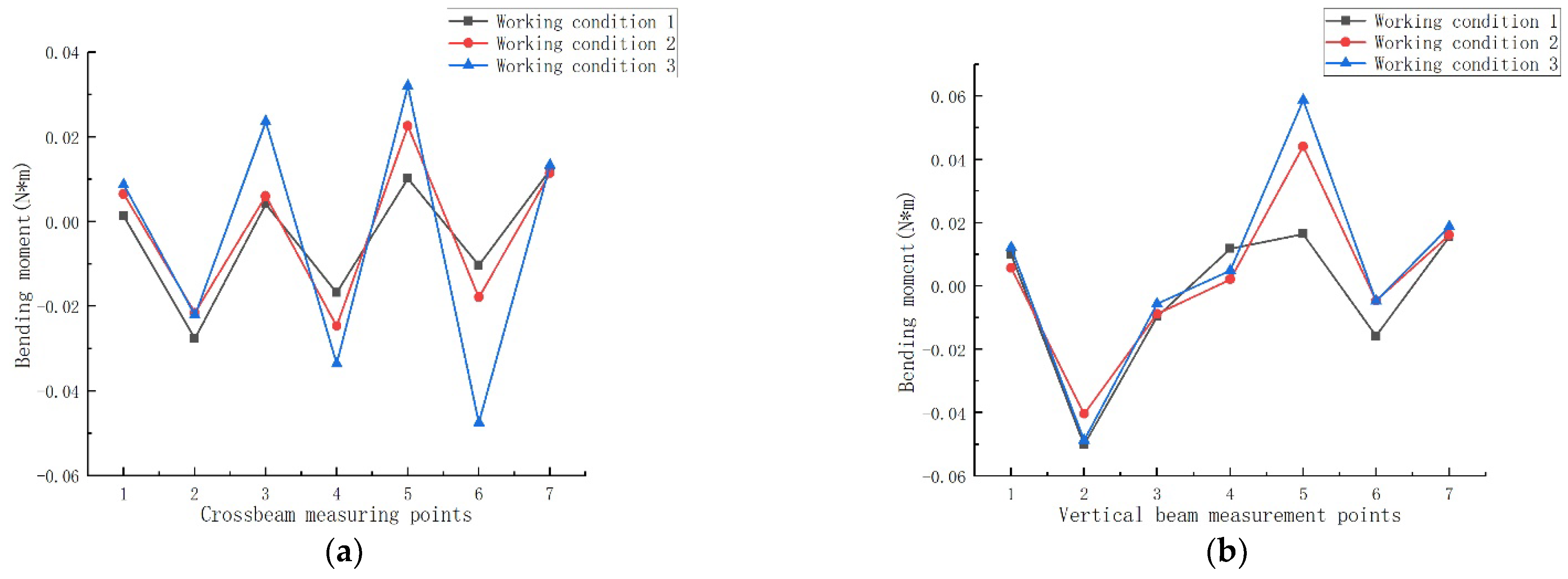
Under different frequency loadings, the bending moments at various points of Rods B and C are shown in Figure 18. The lower parts of Rod segments B1–B3 experience tension, resulting in positive bending moments, while the upper parts of Rod segments B3–B5 are under tension, creating negative bending moments. There is a tendency for the surrounding soil to slide downwards, with the maximum bending moment occurring at the anchor head.

The bending moments in Rod C exhibit an alternating tensile pattern, resembling a wave-like bending behavior. Rod segments C1–C3 and the lower part near the anchoring end experience tension, generating positive bending moments and causing the soil around these segments to compact. Conversely, from Rod segment C3 to the upper part near the anchoring end, tension results in negative bending moments, leading to a tendency for the surrounding soil to slide downward. The maximum bending moment is observed at Rod C5.

The bending moments at various points of Rods B and C increase with the rise in frequency, but in comparison to axial forces, the overall bending moments in these rods are relatively small.

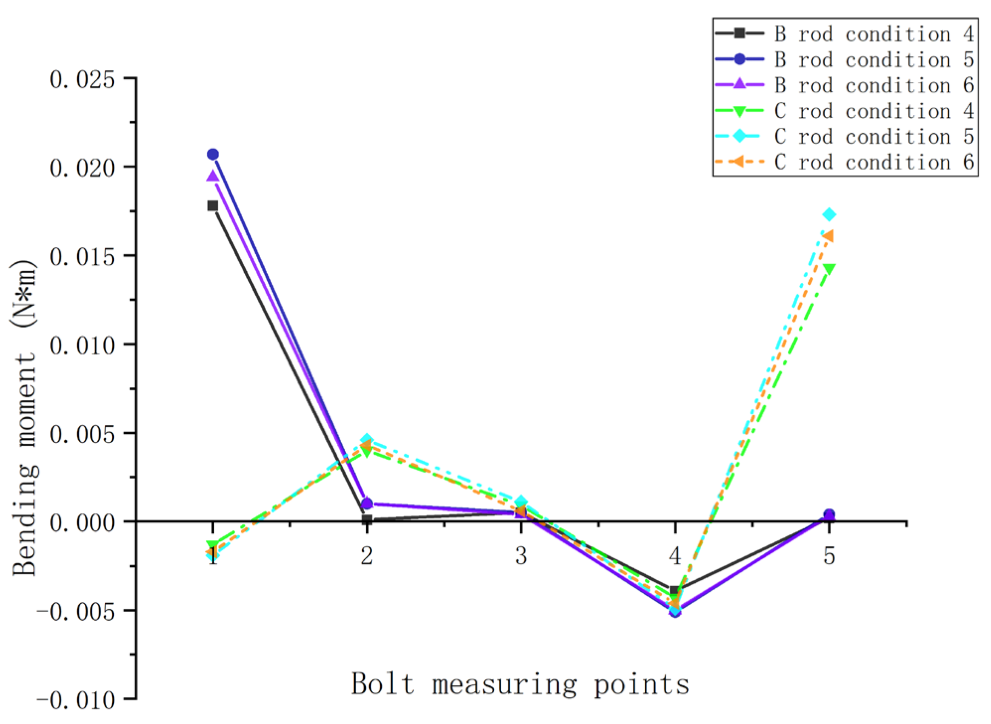
According to the statements in academic journals, the bending moments at various measuring points for Bars B and C under different peak loads are shown in Figure 19. At the lower section of Bars B1–B2, tension generates positive bending moments, while at the upper section of B2–B5, tension creates negative bending moments. The soil around the body bars of B near the anchor head is compacted, indicating a tendency for possible slippage of the soil near the anchor head.

For Bar C, segments C1–C3 and the lower part near the anchor end experience tension, resulting in positive bending moments, whereas from C3 to the upper part near the anchor end, tension generates negative bending moments. The maximum bending moment for Bar B occurs at the anchor head, whereas for Bar C, it appears at the anchor end. With an increase in the peak values of loading, both Bars B and C exhibit only a slight increase in bending moments.

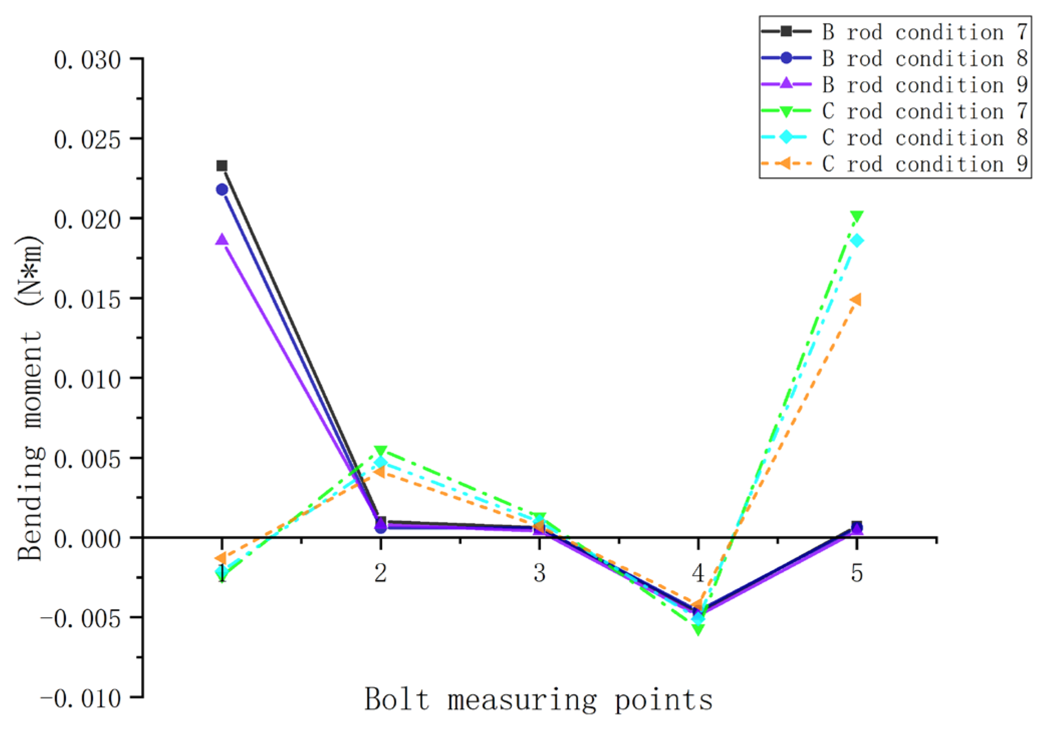
Under different maximum peak loadings, the bending moments at various points of Rods B and C are illustrated in Figure 20. The lower sections of Rod B segments B1–B3 are under tension, resulting in positive bending moments and leading to soil compaction around the rod tip. Conversely, the upper parts of Rod segments B3–B5 are under tension, generating negative bending moments and causing a tendency for the surrounding soil to slide.

Rod C exhibits an alternating tensile pattern, resembling a wave-like bending behavior. Rod segments C1–C3 and the lower part near the anchoring end experience tension, generating positive bending moments, while from Rod segment C3 to the upper part near the anchoring end, tension results in negative bending moments. Rod C might exhibit significant bending deformation at C3, where the surrounding soil around the front part of C3 is compacted, while the soil around the rear part shows signs of sliding. The maximum bending moment occurs at point B1 for Rod B and at point C5 for Rod C.

As the maximum peak loading increases, only the maximum bending moment point, B1 in Rod B, decreases. In contrast, the bending moments at various points in Rod C decrease as the maximum peak loading increases.

Compared to the axial forces on the anchor rods, the bending moments on the anchor rods are considerably smaller. With an increase in depth, the point of maximum bending moment on the anchor rods also shifts from the anchor head towards the anchoring end. The bending moments along the length of the anchor rods exhibit an alternating tensile pattern resembling waves. Near measurement point 3, the soil around the segment close to the anchor head is compacted, while in the vicinity of the segment close to the anchoring end, there is a tendency for the soil to slide, indicating the potential presence of a slip surface near the anchoring end of the anchor rods.

The bending moments are significantly influenced by the loading frequency, increasing with higher loading frequencies. However, the influence of varying maximum peak loads on the bending moments is relatively small, showing only minor fluctuations in the bending moments. The impact of the maximum peak load on the bending moments is more evident, with the bending moments decreasing as the maximum peak load increases.

3.5. Wooden Frame Beam Bending Moment Analysis

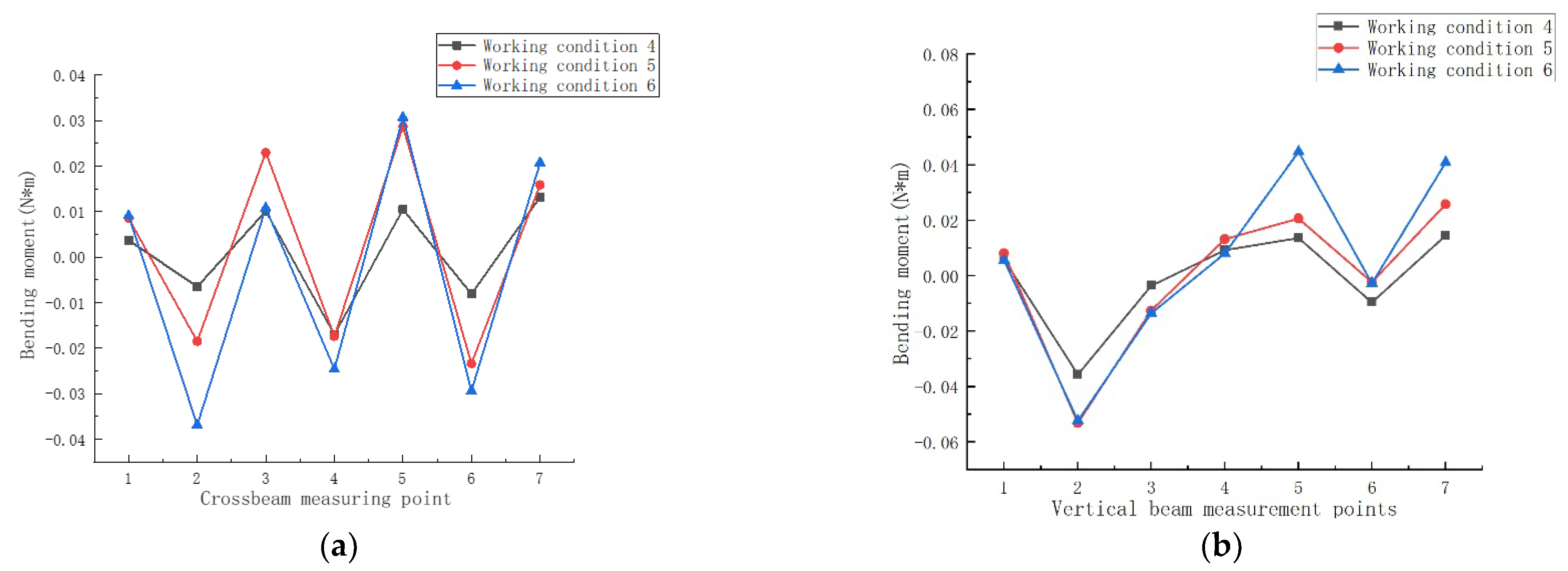
The bending moments at various measuring points of the frame beams under different loading frequencies are illustrated in Figure 21. For the horizontal frame beams subjected to top loading, the lower sections of measuring points H1, H3, H5, and H7 are under tension, indicating positive bending moments, while the upper sections of measuring points H2, H4, and H6 are under tension, indicating negative bending moments. As the frequency increases, the bending moments at each measuring point gradually increase, with larger amplitudes at higher frequencies.

Regarding the vertical frame beams under loading, the lower sections of segments S4–S7 are under tension, indicating positive bending moments, whereas the upper sections of segments S1–S4 are under tension, indicating negative bending moments. With the frequency increase, segment S5 exhibits a significant increase in bending moment, reaching the maximum, while segments S2, S4, and S6 show slight increases in bending moments, and the remaining measuring points remain relatively stable.

Comparing the two diagrams, both horizontal and vertical frame beams exhibit an alternating pattern of tension in bending moments. The bending moments of the horizontal beams are more affected by the loading compared to the vertical beams.

The bending moments at various measuring points of the frame beams under different upper and lower peak values of loading are illustrated in Figure 22. The overall bending moments exhibit an alternating pattern of tension, resembling a wave-like shape. With the increase in upper and lower peak values, except for H3, the bending moments at the remaining measuring points significantly increased. The bending moments at the sides of the beam are relatively smaller and show less variation.

For the vertical frame beams under loading, the lower sections of segments S4–S7 are under tension, indicating positive bending moments, while the upper sections of segments S1–S4 are under tension, indicating negative bending moments. With the increase in upper and lower peak values, the bending moments at each measuring point notably increase.

The bending moments at various measuring points of the frame beams under different upper peak values of loading are illustrated in Figure 23. Under the loading conditions, the lower parts of the horizontal beam at points H1, H3, H5, and H7 are under tension, while the upper parts at points H2, H4, and H6 are also under tension. With the increase in upper peak values, there is a significant increase in bending moments at points H3, H4, and H6, while the bending moments at points H1, H2, and H7 decrease. For the vertical beam, the lower sections of segments S4–S7 are under tension, and the upper sections of segments S1–S4 are under tension. The change in bending moments with the increase in upper peak values is minimal.

Both the horizontal beam and the vertical beam of the wooden frame beams exhibit a wave-like pattern of alternating tension and compression. This behavior resembles the actual structural bending observed in frame beams in engineering practice. Within the combined system of slope soil, bamboo anchor rods, and frame beams, the frame beams experience a dual compression–tension stress pattern. The horizontal beam mainly experiences bending stress in the middle and anchor head sections, suggesting a need for reinforced support in the midsection for engineering purposes. The vertical beam shows upward tension and outward bending in the upper section, while the lower section experiences downward tension and inward bending toward the slope face. The horizontal beam is notably affected by changes in frequency, upper and lower peak values, and peak value differences.

4. Stability Analysis of the Slope of Roadbed Supported by Timber-Frame Beam–Bamboo Anchor Rod

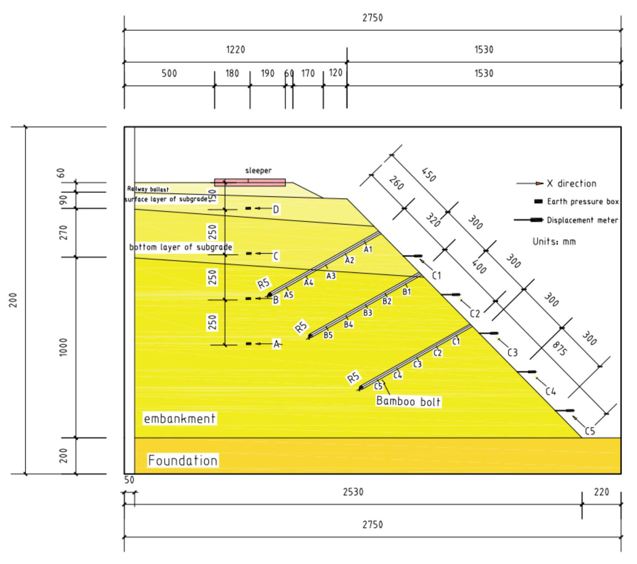
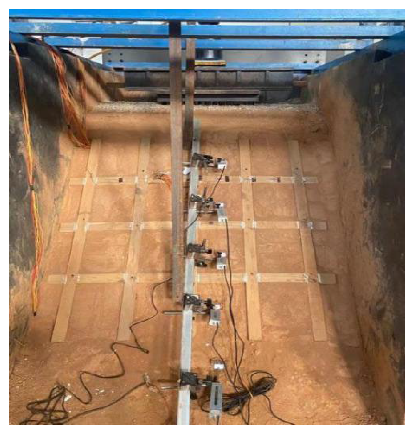
The slope model is divided into five soil layers, consistent with the parameters of the indoor physical model test, comprising the foundation layer, embankment layer, sub-base bottom layer, sub-base surface layer, and ballast layer. The experimental slope’s dimensions were scaled up at a similarity ratio of 1:7 to establish a full-scale model of the road slope supported by wooden frame beams and bamboo anchor rods. The bamboo anchor rods were arranged in a pattern of three rows and three columns, embedded at an angle of 105 degrees, while the wooden frame beams were arranged in four rows and five columns, both using 1D embedded beam elements. The slope soil adopted the Mohr–Coulomb model, and the bamboo anchor rods and wooden frame beams were modeled using elastic elements. After generating the solid and dividing it into grids, the model is depicted in Figure 24.

4.1. Slope Safety Factor

The slope safety factor is an essential indicator of slope stability. Midas GTS NX calculates the slope safety factor by iteratively reducing the internal friction angle and cohesion of the slope soil using the strength reduction method. When the slope approaches the critical point of failure, the value by which the slope is reduced represents the safety factor of the slope.

Table 4. Coefficient of safety of slopes with different number of rows.

Side Slopes	Safety Factor K	Safety Factor Improvement Rate
Unsupported slope	1.103	-
Three rows and three rows of bamboo anchor slope	1.325	20.13%

shows the safety factor of the roadbed slope under different numbers of bamboo anchor supports in loading condition 2. Under the action of train loads, the safety factor of the roadbed slope significantly increases with the presence of wooden framework beams and bamboo anchor supports. Compared to the safety factor of the roadbed slope without wooden framework beams and bamboo anchor support, there is a 20.13% increase in the safety factor of the slope. This result indicates that the supporting structure effectively reduces the impact of cyclic train loads on the roadbed slope, thereby enhancing its stability.

4.2. Maximum Shear Strain of the Slope

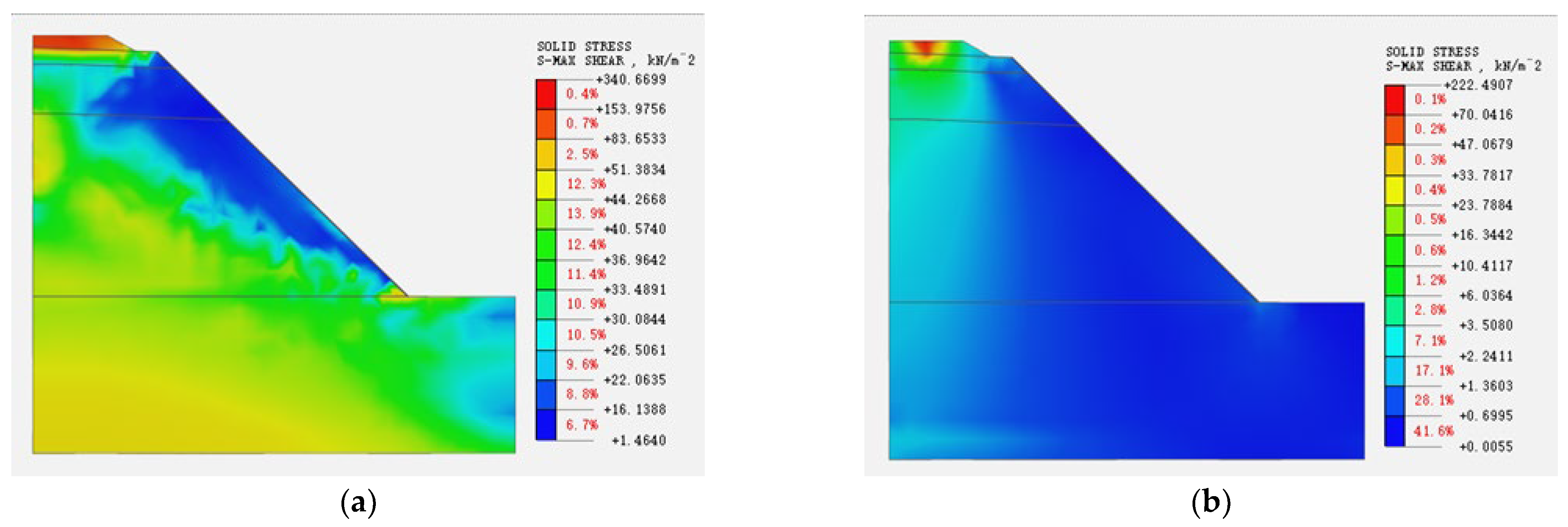
The maximum shear strain of the slope is an important index to measure the force condition of the soil body of the slope, and the dynamic response of the soil body of the slope under train loading can be inferred from the maximum shear strain of the slope to infer the potential slip surface or damage location of the slope. After calculation by Midas GTS NX 2016 finite element software, the cloud diagrams of the maximum shear strains of the embankment slopes under train loads were extracted for different arrangements of bamboo anchors and wooden frame beam support arrangements. Figure 25a shows that the maximum shear strain of the slope is distributed at the foot of the slope when there is no wood frame beam–bamboo anchor support, and the potential slip surface is formed with the bed surface at the top of the slope, and the slope is most prone to shear damage at the foot of the slope. Figure 25b shows that when the slope is supported by bamboo anchors and wooden frame beams, the maximum shear strain of the slope appears below the loading place at the top of the slope, and the maximum shear strain of the slope gradually spreads and expands to the slope body from the loading place at the top of the slope, and the shear strain decreases greatly. The maximum shear strain at the foot of the slope is very small, and a potential slip surface is not formed in the body of the slope.

In summary, compared with the maximum shear strain cloud diagram of the unsupported embankment slope, the maximum shear strain is obviously smaller when the slope is supported, and the maximum shear strain is also very small in the area of the slope supported by bamboo anchors and wooden frame beams; the maximum shear strain at the foot of the slope decreases significantly, and there is no through maximum shear strain slip surface formed in the slope, and the range of the distribution is also reduced. This shows that the maximum shear strain distribution range and size of the slope can be greatly reduced in the wooden frame beam–bamboo anchor support, reducing the probability of shear damage at the foot of the slope, effectively supporting the slope, and improving the stability of the slope.

4.3. Maximum Shear Stress on the Slope

The maximum shear stress of the slope is also one of the important indices to judge the stability of the slope. Figure 26a shows that when the slope is unsupported, the maximum shear stress peak is mainly concentrated in the ballast layer, and the top and foot of the slope are also subject to large shear stresses according to the potential sliding surface of the slope. At this time, the foot of the slope and the top of the slope are susceptible to shear damage. Figure 26b shows that when the slope is supported by bamboo anchors, the maximum shear stress of the slope decreases abruptly, and the peak shear stress decreases by 34.7%. In the slope supported by bamboo anchors, the maximum shear stress decreases abruptly, and the shear stress is mainly concentrated at the top of the slope below the loading point. It is an arc-shaped downward decay; the foot of the slope and the top of the slope shear stress decrease abruptly, and the probability of occurrence of shear damage is greatly reduced.

In summary, when the slope is unsupported, the maximum shear stress distribution range fills the whole slope, shear damage easily occurs at the top and foot of the slope, and the stability of the slope is poor. Further, when the slope is supported by bamboo anchors and wooden frame beams, the maximum shear stress distribution range of the slope is rapidly reduced and mainly concentrates in the arc-shaped spreading attenuation below the loading point and attenuation mainly concentrates in the ballast layer and the foundation layer, the foot of the slope and the top of the slope shear stress is suddenly reduced, and the probability of shear damage is greatly reduced.

5. Conclusions

This paper conducted model experiments on roadbed slopes that were supported by wooden framework beams and bamboo anchor systems under train loads. Three-dimensional numerical simulations were performed to analyze the effect of train load frequency, peak difference, and peak value on the soil pressure of the roadbed slope. They also analyzed the horizontal displacement of the slope surface, the internal forces within the supporting structure, and the slope safety factor. The relevant conclusions are as follows:

(1)

When the loading frequency increases from 2 Hz to 3 Hz, there is a considerable increase in soil pressure; however, further increments in the loading frequency result in a smaller increase in soil pressure. The increase in dynamic load shows a positive correlation with soil pressure.

(2)

In indoor slope model experiments, the axial force on the anchor rods is not uniformly distributed. Therefore, in engineering design, the assumption of uniform axial force distribution along the length of the anchor rods is deemed unreasonable. Across various conditions, the axial force on the rod tends to be greater closer to the top of the slope. The support system primarily operates with the top-slope anchor rods and then gradually transitions to the anchor rods in the middle and at the foot of the slope. The combined action of the anchor rods and wooden framework beams forms an integral support system that resists slope movement, thereby enhancing slope stability.

(3)

The point of maximum bending moment in the anchor rods gradually transitions from the anchor head to the anchored end with increased burial depth. The bending moment is significantly influenced by loading frequency, increasing with higher loading frequencies. It shows minor fluctuations with variations in upper and lower peak values. Notably, the bending moment is prominently influenced by increased upper peak values, exhibiting a decrease with their rise. This phenomenon might be due to the larger peak difference, causing the combined wooden framework beam–bamboo anchor support system to resist slope movement.

(4)

When employing the wooden framework beam–bamboo anchor support as temporary support in engineering applications for roadbed slopes, it is crucial to monitor and protect the positions at the slope’s top and bottom. Additionally, enhancing the overall integrity of the wooden framework beam–bamboo anchor support is recommended.

(5)

Under the influence of train loads, the roadbed slope with wooden framework beam–bamboo anchor support effectively mitigates the impact of dynamic train loads. The safety factor of the roadbed slope is increased by 20.13% compared to the unsupported condition, significantly enhancing slope stability.