Decision Support System Driven by Thermo-Complexity: Scenario Analysis and Data Visualization

Abstract

The present modelling aims to construct a computational information representation system useful for decision support system (DSS) solutions in the realization of intelligent systems or complex systems analysis solutions. Starting from an n-dimensional space (with n ≥ 7) represented by problem variables (referred to as CSF—Critical Success Factors), a dimensional embedding procedure is used to transition to a two-dimensional space. In the two-dimensional space, thanks to new lattice motion algorithms, the decision support system can determine the optimal solution with a lower computational cost based on the decision-maker’s preferences. Finally, thanks to an algorithm that takes into account the hierarchical order of importance of the seven CSFs as per the expert’s liking or according to his optimization logics, a return is made to the n-dimensional space and the final solution in the original space. As we will see, the starting and ending states in the n-dimensional space (referred to as micro-states) when projected into the two-dimensional space generate states (referred to as macro-states) which are degenerate. In other words, the correspondence between micro-states and macro-states is not one-to-one, as multiple micro-states correspond to one macro-state. Therefore, in relation to the decision-maker’s preferences, it will be the responsibility of the decision support system to provide the decision-maker with the micro-state of interest in the n-dimensional space (dimensional emergence procedure), starting from the obtained optimal macro-state. This result can be achieved starting from a flat chain of sensors capable of measuring/emulating certain specific parameters of interest. As we will see, it emerges that by considering random–exhaustive rolling value paths in order to track and potentially intervene to rebalance a dynamic system representing the state of stress/sensing of a system of interest, we are using the most general and, therefore, complex hypotheses of ergodic theory. In this work, we will focus on the representation of information in n-dimensional and two-dimensional spaces, as well as construct evaluation scenarios. We will also show the results of the decision support system in some cases of specific interest, thanks to a specific lattice motion algorithm of the realized decision-making environment.

1. Introduction: DSS Short Overview

Starting from the first book on decision support systems (DSS) in 1978 by Keen and Scott Morton, many methodological, technological, and applicative works have been carried out over the last 50 years [1]. Over the years, many interpretations and application instances have followed one another in most operational areas, from the technical–scientific context, governance, management, production, strategic analysis, in medical and health contexts, in logistics and transport, defense, security, cybersecurity, and practically everywhere. The concept of DSS was first defined by M.S. Scoot Morton as a management decision system (MDS) [2], but in the following years this type of solution has increasingly become an interactive computer-based solution to help any decision-maker who uses a large amount of data and information to solve unstructured problems, i.e., problems with a large number of variables, or with uncertainty or info-incompleteness [3]. As reported in [4] a way to classify DSSs is if they are (i) document driven, (ii) model driven, (iii) communication driven, (iv) data driven, and (v) knowledge driven. As highlighted in [5], most current DSSs are limited to merely finding the situation, that is, a kind of diagnostics, and do not have a unified integrated mechanism to offer adequate solutions. Furthermore, we can add that, among the DSSs which offer adequate solutions, it is very difficult to find computational systems that offer decision-making paths and not only target solutions. The aim of this work is above all to shift the focus to the decision-making path and not to be a survey of the different decision support systems. Therefore, just for the sake of completeness, and for better framing the topic we intend to deal with, below we find some useful references to learn more about the different types of decision support systems. A document-driven decision support system (DSS) is a type of information system that utilizes documents and textual data to facilitate decision-making processes within an organization [6,7,8,9,10,11,12,13,14,15]. A model-driven decision support system (DSS) is a computer-based system that helps organizations and individuals make informed decisions utilizing mathematical models and simulations [16,17,18,19,20,21,22]. A communication-driven decision support system (DSS) is a type of DSS that emphasizes the importance of effective communication among decision-makers and stakeholders [16,17,21,22,23,24,25,26]. A data-driven decision support system (DSS) is a computer-based tool or system that utilizes data and analytical models to help individuals and organizations make informed decisions. These systems are designed to collect, process, and analyze data to provide insights, predictions, and recommendations for decision-making [12,16,17,23,27,28,29,30,31,32]. A knowledge-driven decision support system (DSS) is a type of computer-based information system that aids decision-makers by providing access to and utilization of knowledge resources [33,34].

The solution we present in this paper is a model-driven DSS. The modelling takes place in the context of complexity theory, and it is inspired by thermodynamics and statistical mechanics. In fact, just as in thermodynamics state variables such as entropy and energy are defined to represent many variables of systems, also in this work we will project states represented by several variables in a space with two variables, calling the first micro-states and the second macro-states of the system under study. As we shall see, the goal of such a size reduction is the significant reduction of computational cost, but we would then have to solve the problem of returning to the initial multi-variable space (i.e., the space where micro-states live) since the micro-state represented by energy and entropy are degenerates.

2. Critical Success Factors and Hyperspace

What we now call chaos and complexity theory was initially produced under the name “ergodic theory”, as the term “chaos theory” was introduced only in the mid-twentieth century. Ergodic theory primarily deals with the mathematical study of the long-term average behavior of dynamic systems. As known from Greek, “érgon” means energy, and “odòs” means road or path. Therefore, Ludwig Boltzmann and later Josiah Gibbs introduced this term in reference to complex mechanical systems that were attributed the property of assuming all microscopic dynamic states compatible with their macroscopic state during their spontaneous evolution [35]. In other words, one macroscopic state could correspond to multiple microscopic states. As we will see, by introducing two state variables, such as the internal energy E of a system (understood as systemic dynamics) and entropy S (understood as imbalance or disorder in a system), a given pair (S, E) will correspond to multiple states of the system at a given space–time location. In order to achieve this goal, the following seven indexes are introduced, and the following target functions are defined and implemented. Indexes (or CSF—Critical Success Factor) representative for the definition of conservative structures: X₁—CSF 1, X₂—CSF 2, X₃—CSF 3, X₄—CSF 4, X₅—CSF 5, X₆—CSF 6, X₇—CSF 7.

This solution was inspired by a specific need, i.e., the monitoring and supervision of a specific area of interest in order to create a decision support system for physical security; the analysis of potential criminogenic phenomena; and the enhancement of urban territory. In fact, in this specific application of the methodology that we will analyze in this work, the seven CFS are, respectively, a (1) demographic index, (2) environmental index, (3) economic index, (4) organizational index, (5) political index, (6) psychological index, and (7) ethical index. Therefore, considering a specific urban or extra-urban area, thanks to the demographic index, it is possible to have the population density under control; thanks to the environmental index, the criminological aspects are analyzed; the economic index provides an estimate of economic development; with the organizational index the presence of infrastructure is analyzed; thanks to the political index the actual presence and proximity to the population of government and local institutions is considered; the psychological index analyses how the territory is perceived by the population; and the ethical index considers quality of life in relation to value systems and cultural traditions. The psychological index analyzes how the territory is perceived by the population, while the ethical index considers the quality of life in relation to value systems and cultural traditions. As we will see at the end of this article, the suggested dynamics of the seven CSFs indicated above are used for the control of the urban territory of a large city with high complexity, using a smart city perspective as we will see. This experimentation showed the generality and the level of abstraction of both the model and the application solutions. Therefore, the system has been generalized to be applied to other contexts thanks to the identification of the different CSFs chosen on a case-by-case basis.

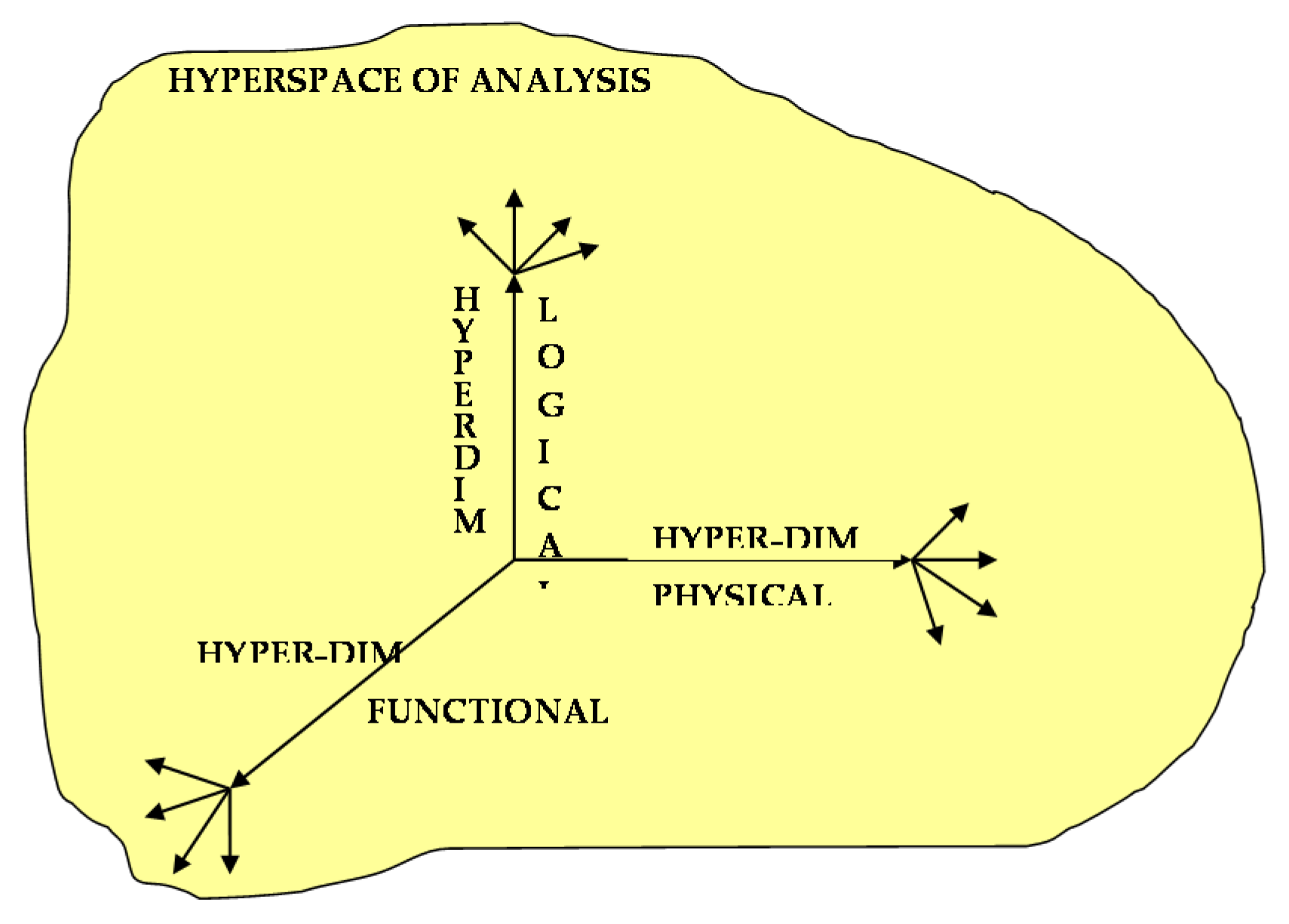
As we will see, the underlying model proposed below uses n-dimensional spaces as described hereinafter. Methodologically, in order to identify operational strategies and systematically analyze the multifaceted complexity of the CSFs at play, it is necessary to conduct an analysis in a hyper-space constructed based on three distinct hyper-dimensions: the (i) physical hyper-dimension, (ii) logical hyper-dimension, and (iii) functional hyper-dimension. In this scenario, the hyper-dimensions are characterized by a multi-dimensional space where each dimension is associated with one or more parameters.

We define hyper-space as the structured n-dimensional space whose dimensions are represented by the physical, logical, and functional hyper-dimensions (see Figure 1).

Such an analysis has the advantage of having a mathematical representation that allows for qualitative assessments, as is the case with other approaches, and also possesses significant quantitative expressive power. Indeed, if we associate a numerical value x, ranging from 0 to 1 (i.e., within a given sustainability range), if x ∊ [0, 1]⊂ℜ, to each of the parameters at play, represented by a specific dimension of our hyper-space, we will be able to make quantitative estimates of the situation under study. This will help us to identify the best actions to take. Furthermore, such a method, which mathematically falls under the so-called fuzzification processes, i.e., processes that remap the possible values of a given quantity to an interval (0,1), has the advantage that if we associate the value zero with the impossible event and the value one with the sure event, a given event with an intermediate probability will have a likelihood P of occurrence precisely equal to the percentage value x ∊ (0,1). At this point, for the analysis of a given phenomenon, classical tools of probability and inferential statistics can be used, through the use, for example, of composite or conditional probabilities to describe complex phenomena or activities. Alternatively, innovative mathematical methodologies can be used to describe complex, stochastic, and self-similar phenomena, such as fractals, self-similar stochastic dynamic processes, Markov chains, and multiscale and multiresolution analyses. In this approach, a given event becomes a point associated with a set of CSFs and probabilities in this multidimensional space (hyper-space), which is both a state space and an event space. Conversely, a given phenomenon will be mathematically represented by a set of transitions from one state to another. Analyzing the parameters related to subsequent states methodologically allows for both a contextual and scenario analysis (deductive approach) and a predictive analysis (inductive–experiential simulated approach). It is easy to understand that such a methodology focuses on the event and its dynamics. It is evident, therefore, that such an approach is more effective in terms of description and prediction, allowing for the identification of more efficient prevention and mitigation actions compared to a more traditional analysis of a given situation, where aspects such as forms or manifestations, etc., of the situations themself are analyzed. Thanks to such a model, it will be possible to implement management strategies which realize a decision support system (DSS). These CSFs represent the independent variables of the computational model, and, therefore, their values will be collected or emulated for analyses and study. The CSFs can take on six distinct values, namely X_i = 0,1,2,3,4,5 with i = 1, …, 7. The values assumed by the CSFs will have the following meanings, providing the following semantic modelling values: 0—not acquired/not emulated, 1—low, 2—low–medium, 3—medium or normal, 4—medium–high, 5—high. The n-tuple (X₁, X₂, X₃, X₄, X₅, X₆, X₇,) precisely represents the state of the system at a given time. From the perspective of advanced modelling, the network of sensors/emulators can be likened to a chain of harmonic oscillators. Their oscillations can be either harmonic, leading to energy conservation, or anharmonic, leading to energy dissipation. The value 3 corresponds to a system where the considered parameter is balanced and leads to equilibrium laws and conservation of dynamic systems. Values 2 and 4, on the other hand, represent a system with alteration and energy dissipation and a relative increase in its entropy, the first with implosive trends (i.e., 2) and the second (i.e., 4) with explosive trends. Finally, values 1 and 5 represent systems characterized by parameters far from equilibrium, strongly anharmonic and dissipative, and thus with high entropy, the first (i.e., 1) being close to implosion/freezing and the second (i.e., 5) being close to explosion. Zero indicates a lack of information; therefore, the proposed method and the implemented computational system will manage partial and incomplete information through target functions by formulating hypotheses for statistical inference to support decisions.

3. Target Functions

In this section, we introduce various target functions, abbreviated as STF—System Target Function, useful for achieving the goal.

The main targets to pursue are as follows:

(1)

Knowledge of the system’s state and the situations active on it;

(2)

Completeness and, therefore, the reliability of the information acquired through georeferencing information and the temporal localization of events;

(3)

The ability to associate and contextualize events within classifiable scenarios, allowing for the identification of the following:

(3.1)

Decision strategies (DS);

(3.2)

Management strategies (MS);

(3.3)

Operational strategies (OS).

The mathematical formulation of the problem can be presented in two different types and with different levels of abstraction. A very advanced and extremely realistic modelling should consider memory effects, which, from a modelling point of view, imply the presence of first-order (or even higher) derivative terms for the variables at play, i.e., X_i. Conversely, a simpler approach is typical of control theory, which often stops at formulation in terms of linear combinations. In other words, we are assuming that we do not know the exact f and are analyzing it at different levels of approximation (non-linear in the first case, linear in the second). Regarding the level of abstraction, as we will see, in a first approximation, we will deal with an $f:X\subset {\mathbb{R}}^{10}\to Y\subset {\mathbb{R}}^7$, but from a more refined analysis, it is understood that such a function lives in a weighted Sobolev space H^2,2_G, where G is an appropriate weight. In fact, concerning the components of f, if we consider the first one, which represents “knowledge of the state of the system and the situation active on it”, it is important to know both how the rate ($f_1^{\prime }$) varies and how this variation ($f_1^{″}$) varies. Since we want these functions not to diverge from the norm, they must be square-summable. Furthermore, needing weighted spaces explains why it is necessary to consider H^2,2_G. It is also evident that for complete use of the model, historical information will also be necessary to create a system that is both adaptive and contextualized to support decision-making. Going into implementation details, we define the first target function STF_1 = f_{1 i}n (1) and (2) as follows:

$$f_1:A\times \dots \times A\subset {\mathbb{R}}^7\to B\times C\subset {\mathbb{R}}^2$$

(1)

where $A=\left\{0,1,2,3,4,5\right\}\subset \mathbb{N}$ e $B=\left[0,12\right]\subset \mathbb{N}$, $C=\left[7,35\right]\subset \mathbb{N}$. From a computational point of view, we have

$$f_1=(E,S)=(\frac{1}{7}{{\displaystyle \sum }}_{i=1}^7{\alpha }_i{X}_i,\frac{1}{7}{{\displaystyle \sum }}_{i=1}^7{\alpha }_i\left|X_i-\stackrel{\sim }{X}\right|)$$

(2)

where E represents the internal energy of the system represented by the considered state, S is its Entropy, $\stackrel{\sim }{X}$ is the median, and the coefficients ${\alpha }_i$ are suitable normalization coefficients, defined as follows:

$${\alpha }_i=\frac{{\beta }_i}{5}$$

(3)

with ${\beta }_i$ as the activation parameter (or relative weight), and as such, ${\beta }_i\in \left[0,1\right]\subset \mathbb{R}$.

In the absence of historical information, we assume ${\beta }_i=1$, and it is also possible to choose not to normalize (i.e., multiply by 1/7), as we will do later for simplicity, without a loss of generality. Formally, it is common to say that $f_i\in BV\left(0,1\right),$ where BV is the space of functions with bounded values in the interval $\left[0,1\right]\subset \mathbb{R}$. The choice of the aforementioned interval comes from the fact that, this way, the target function f₁ will return a value between zero and one, which can be directly associated, through a fuzzification process, with a probability of incidence of the CSFs on a specific systemic alteration. Therefore, the STF function f₁ responds to the first objective, i.e., knowing the state of the system and the situations active on it. As mentioned earlier, a more accurate model could also include higher-order powers in the X_i variables or derivative terms. However, considering the almost complete absence of linear models similar to the one considered, we prefer not to further complicate the modelling in this context. The STF f₁ function, by construction, does not address the second objective, i.e., the temporal and geospatial localization of information. To meet this requirement, a generalization of the function is necessary. In this regard, in (4), we introduce the following function, STF_2 = f₂, defined as follows:

$$f_2:T\times P\times A\dots \times A\subset {\mathbb{R}}^{10}\to T\times S\times B\times C\subset {\mathbb{R}}^5$$

(4)

where T represents the temporal domain and P the spatial domain defined using the two coordinates, latitude and longitude, provided using GPS. This function allows temporal and spatial resolution of events. From a computational perspective, we can find the function of 10 real variables in a five-dimensional space over a set of real numbers, i.e., a vector-valued function as follows:

$$f_2=\left(f_{2,1},f_{2,2},f_{2,3}\right)$$

(5)

where

$$f_{2,1}=t$$

(6)

with t being the temporal parameter belonging to the domain T,

$$f_{2,2}=\left(long, lat\right)$$

(7)

with (long, lat) being the GPS georeferencing coordinates,

$$f_{2,3}=f_1.$$

(8)

Through construction, the STF f₂ function in (4) addresses the first two objectives. It could happen that the decision-maker does not provide complete information, i.e., information about all seven pointers. This could happen for various reasons, such as

-

There is a need for rapid intervention, so only the most significant alterations are reported;

-

There are significant alterations in only CSFs, and the others are not reported;

-

Etc.

The results will be overly complex for the system, which will have to managed incompletely and using partial information. Therefore, to address this complexity, the model needs to account for it. Specifically, the system will associate a value of zero with the missing CSFs, which will automatically imply necessary freezing of the CSFs at the previously introduced values in the subsequent historical data. While this solves the problem of managing input, it does not provide an exhaustive response in terms of services to be prepared for monitoring and analysis. In other words, there is a need to address the third of the three themes considered in the three objectives to which the STFs must be subordinated. To control such aspects of information incompleteness, two output parameters are introduced into the target function, defined as proximity and completeness. Proximity represents the belonging of an output to a given scenario (e.g., equilibrium, explosive, implosive, etc.), so

$$V:A\times \dots \times A\subset {\mathbb{R}}^7\to S_c\subset \mathbb{R}$$

(9)

where $S_c\subset \mathbb{N}$ is the space of admissible scenarios that we will describe later. Completeness provides a level of informational completeness regarding the seven CSFs, and it is defined as

$$C:A\subset \mathbb{R}\to B\subset \mathbb{R}$$

(10)

which computationally can be expressed as

$$C=\frac{n}{7}$$

(11)

where $n$ is the number of CSFs which assume values other than zero. In this way, an answer to the third of the objectives identified at the beginning of the section is also provided. In conclusion, the complete target function to be considered will be STF_3 = f₃ as formally described below in (12):

$$f_3:T\times S\times A\dots \times A\subset {\mathbb{R}}^{10}\to T\times S\times B\times S_c\times B\subset {\mathbb{R}}^7.$$

(12)

In other words, the achievement of the monitoring goal for alterations in the system is obtained through a vector-valued function, i.e., a function of 10 real variables (inputs) that returns a real vector with six components (outputs). The ten inputs are time, latitude, and longitude, and the seven characteristic CSFs, while the six outputs are time, latitude, longitude, the dynamic (i.e., energy) associated with the state, the disorder (i.e., entropy) associated with the state, the resulting scenario, and information completeness. From a computational perspective, we have

$$f=\left(f_1,f_2,f_3,f_4,f_5,f_6,f_7\right)$$

(13)

where $f_1=t$, with t being the temporal parameter belonging to the domain T; $f_2=long$, with long corresponding to GPS georeferencing longitude; $f_3=lat$, with lat corresponding to GPS georeferencing latitude; $f_4=E$, corresponding to the internal energy of STF_1; $f_5=S$, corresponding to the entropy of STF_1; $f_6=m$, where m is one of the scenarios in the Sc space; $f_7=n/7$, where n is the number of pointers that assume values other than zero. Be careful not to confuse STF_3, which is a vector-valued function, with f₃ = lat, which is one of its components. From a formal perspective, using vector notation, this can be written as follows in (14):

f(t, long, lat, X₁, X₂, X₃, X₄, X₅, X₆, X₇) = t e₁ + long e₂ + lat e₃+ E e₄+ S e₅ + m e₆ + n/7 e₇

(14)

where f is the vector field corresponding to the final objective to be monitored, and the e_k vectors with k = 1, …, 7 are the basis vectors of the seven-dimensional vector space of outputs. Starting from this target function, as you will see later, three more complex target functions will be constructed as follows:

-

Target function for the construction of optimal decision strategies, STF_SD;

-

Target function for the construction of optimal management strategies, STF_SG;

-

Target Function for the construction of optimal operational strategies, STF_SO.

The complexity of STF_SD, STF_SG, STF_SO is such that specific subsequent sections are required for a detailed explanation, to which we refer for further elaboration.

4. Representation and Characterization: Scenarios and States

In the previous section, we introduced the set of scenarios. Here, we will summarize the various categories before detailing them. From a mathematical standpoint, the number of possible scenarios is very high; in fact, this number is expressed in terms of permutations with repetition of length 7 from the elements of the set {1,2,3,4,5}, and it is, therefore, given using 5⁷, resulting in 78,125 different scenarios. For analytical purposes, it is convenient to cluster the 78,125 scenarios into classes with common properties. Below, we present a statistical clustering to analyze deviations from the fundamental states. In the next section, a more advanced classification in terms of evolutionary dynamics is presented. The clustering of scenarios into classes plays a crucial role. In this modelling phase, clustering scenarios into classes will allow for the deconstruction of information and the construction of analytical and automatic decision support models in the analysis phase. In other words, using a thermodynamic approach, we will show that the 78,125 scenarios can be seen as microscopic states, each of which can be associated with a much lower number of macroscopic states expressed in terms of state variables such as internal energy (E) and entropy (S). The classes of clustered scenarios using statistical techniques will be indicated with the acronym S#, where the symbol # will be a decreasing progressive number starting from seven. Therefore, one scenario will contain multiple seven-component n-tuples. Each seven-component n-tuple describes a state of the system. The components are the seven characteristic CSFs, X₁, X₂, X₃, X₄, X₅, X₆, X₇, which, once assigned, characterize the state of the system under study. Since systems can have different dynamics based on other parameters such as space or time, it might happen that all CSFs vary simultaneously, or only some of them exhibit gradients, while the rest remain in their previously evaluated state.

The following

Table 1. Scenarios and their characterizations.

Scenario	Scenario Characterization
S7	All 7 CSFs are variable
S6	6 out of the 7 CSFs are variable, and 1 is fixed
S5	5 out of the 7 CSFs are variable, and 2 are fixed
S4	4 out of the 7 CSFs are variable, and 3 are fixed
S3	3 out of the 7 CSFs are variable, and 4 are fixed
S2	2 out of the 7 CSFs are variable, and 5 are fixed
S1	1 out of the 7 CSFs is variable, and 6 are fixed
S0	1 out of the 7 CSFs is variable, and 6 are fixed

summarizes the various possibilities.

Even though it will be subject to further in-depth analyses, it is interesting to anticipate that there is a connection between the aforementioned scenarios and the type of dynamics of the studied system. Thanks to an in-depth modelling activity to better meet analysis requirements, the seven scenarios mentioned in the following section will be reorganized into twelve. However, the following observations remain valid.

Scenario S7 is suitable for describing a system with no memory, meaning that there are no previous observations or it is a system with variable dynamics, where different states are expected with small time or space intervals. Such a scenario is, therefore, a scenario with very high variability from both an energetic and entropic point of view. A priori, it is a scenario that can easily become chaotic.

Scenario S6 shows the emergence of persistence, meaning that one of the seven pointers does not change. This means that an order is beginning to emerge; however, variability is still very high, so we are dealing with systems with high informational entropy and tendencies toward chaos.

Scenario S5 shows a greater level of order compared to previous cases; in fact, we have two fixed CSFs. However, two fixed CSFs compared to five variables still result in the dominance of variability, instability, and disorder over order.

In Scenario S4, we find a slightly unbalanced situation towards disorder, while in S3, order and disorder reverse their roles, meaning that we are dealing with scenarios which contain states with four fixed CSFs and three variables. In other words, in S3, we have a system whose states are more easily predictable; it begins to stabilize over time and takes on a specific characterization.

In S2, the situation has only two CSFs that are variable, so we are dealing with systems that express extremely predictable and orderly dynamics.

Finally, Scenario S1 is a scenario with only one variable; the states contained in it are said to be close to a state of immobilization or freezing.

S0 represents a fundamental scenario, with minimal variation, in which the system tends to remain in its state (frozen system). Below S0, there is immobility, while above S7, there is chaos. Let us start by analyzing Scenario S7 in more detail and then the others; it is the most comprehensive and complex one, representing a partition of the state space with its 5⁷ = 78,125 admissible states.

4.1. S7 Scenario

Scenario S7 can be broken down into 13 subsets of states (or sub-scenarios). These subsets are obtained by considering characterization. By characterization, we mean the different ways in which the n-tuple of the seven CSFs can be obtained, as in

Table 2. S7 sub-scenarios, where the symbol ◊ indicates the composition of the micro-state string as described above.

Sub-Scenario	Characterization	N.Sub-Scenarios	N.States	E	S
S7_1	7	5	5 × (7!/7!) = 5	[7, 35]	0
S7_2	6◊1	20	20 × (7!/6!) = 140	[8, 34]	[1, 4]
S7_3	5◊2	20	20 × (7!/5!2!) = 420	[9, 33]	[2, 8]
S7_4	5◊1◊1	30	30 × (7!/5!) = 1260	[10, 32]	[2, 7]
S7_5	4◊3	20	20 × (7!/4!3!) = 700	[10, 32]	[3, 12]
S7_6	4◊2◊1	60	60 × (7!/4!2!) = 6300	[11, 31]	[3, 11]
S7_7	4◊1◊1◊1	20	20 × (7!/4!) = 4200	[13, 29]	[4, 9]
S7_8	3◊3◊1	30	30 × (7!/3!3!) = 4200	[12, 30]	[4, 12]
S7_9	3◊2◊2	30	30 × (7!/3!2! 2!) = 6300	[14, 29]	[4, 11]
S7_10	3◊2◊1◊1	60	60 × (7!/3!2!) = 25200	[14, 28]	[5, 11]
S7_11	3◊1◊1◊1◊1	5	5 × (7!/3!) = 4200	[17, 25]	[6, 9]
S7_12	2◊2◊2◊1	20	20 × (7!/2!2!2!) = 12600	[16, 26]	[6, 10]
S7_13	2◊2◊1◊1◊1	10	10 × (7!/2!2!) = 12600	[18, 24]	[7, 10]

.

The symbol ◊ indicates the composition of the micro-state string and so for example 6◊1 means that six CSFs are equal, and one is different; 5◊2 means that five CSFs are equal, and two are different but equal to each other; and 4◊2◊1 means that four CSFs have one value, two have another one, and one has yet another one, and so on

The total number of sub-scenarios is 330. This value is calculated using the well-known combinatorial expression for calculating combinations with repetition of n = 5 distinct elements taken k = 7 at a time, which is

$$C_{n,k}=\left(\begin{array}{c}n+k-1\\ k\end{array}\right)=\frac{\left(n+k-1\right)!}{\mathrm{k}!\left(\mathrm{n}-1\right)!}$$

(15)

which in this case becomes

$$C_{5,7}=\left(\begin{array}{c}5+7-1\\ 7\end{array}\right)=\frac{11!}{7!4!}=330.$$

(16)

The sum of the sub-scenarios is indeed 330; however, it contains extra information because the scenario under consideration, with seven CSFs, has been broken down into sub-scenarios of various types, such as seven identical CSFs, six identical, and one different, etc. This breakdown was necessary to calculate the number of states belonging to each sub-space, or using thermodynamic language, to calculate the number of microscopic states corresponding to the same macroscopic state. It is given using the product of the number of sub-scenarios and the number of permutations with repetition of the specific characterization. In other words, to calculate the states, the number of components of the sub-scenario has been multiplied using the following relation

$$P_{k,k_1,k_2,\dots k_r}=\frac{k!}{k_1!k_2!\dots k_r!}$$

(17)

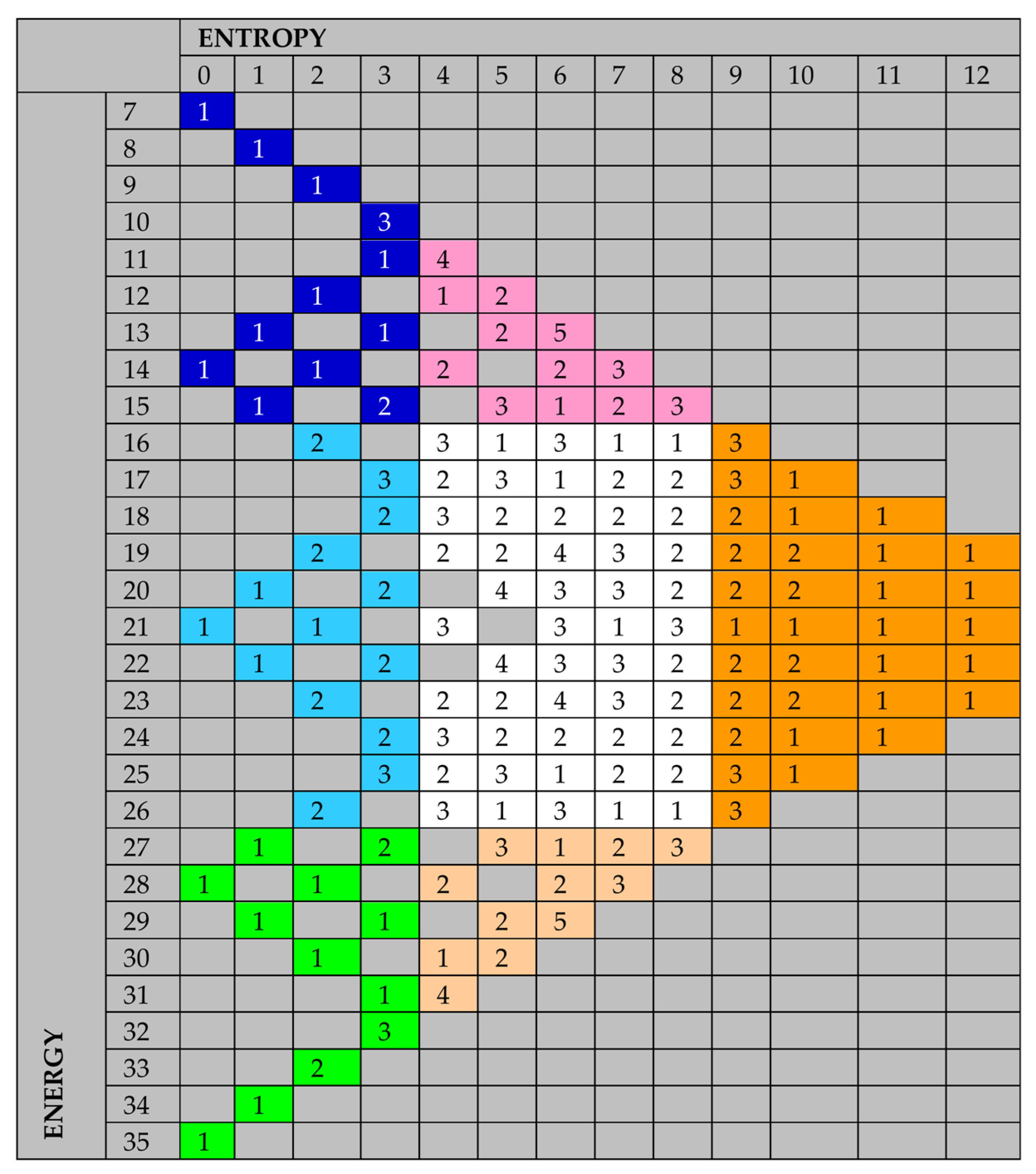
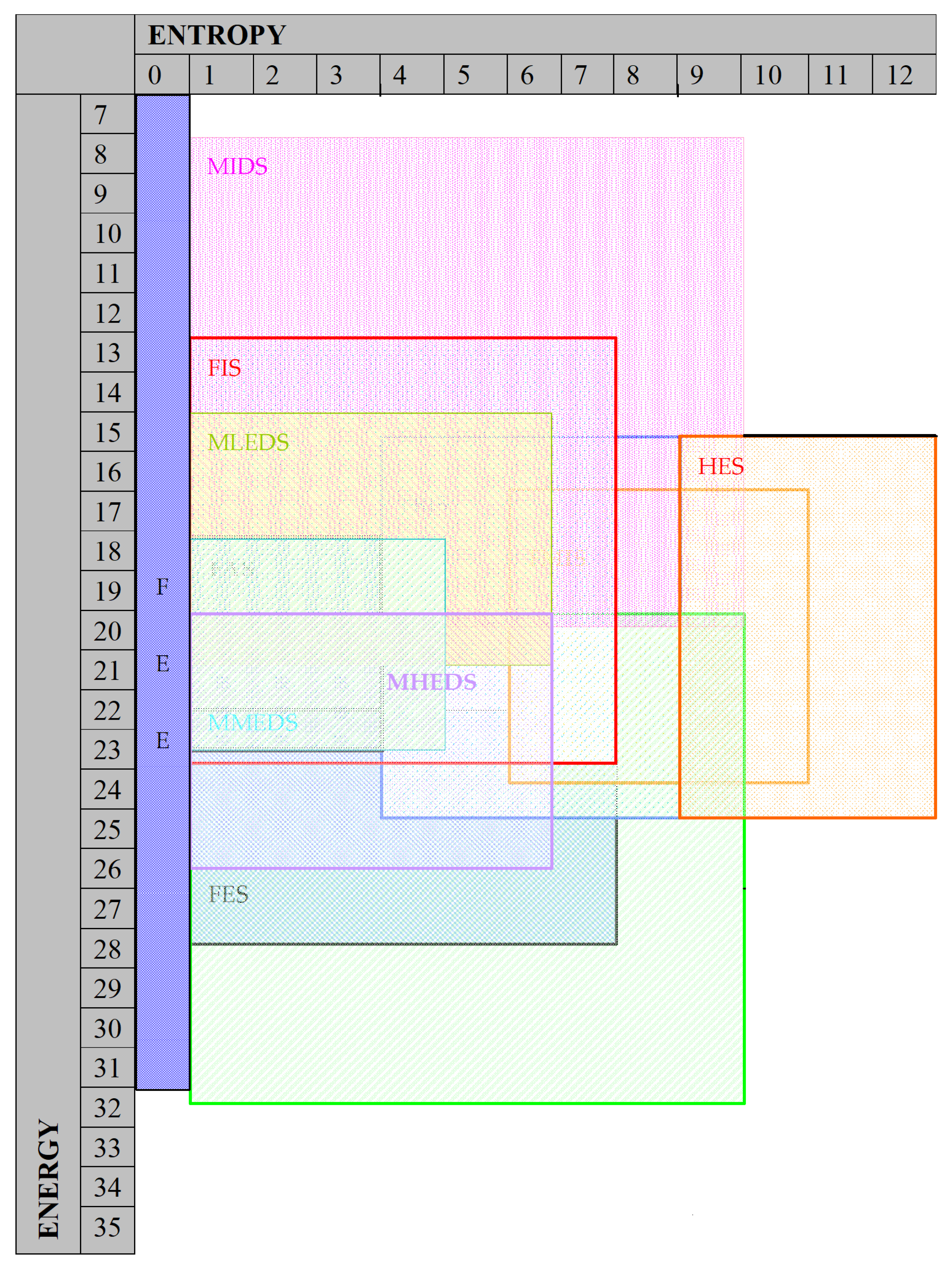
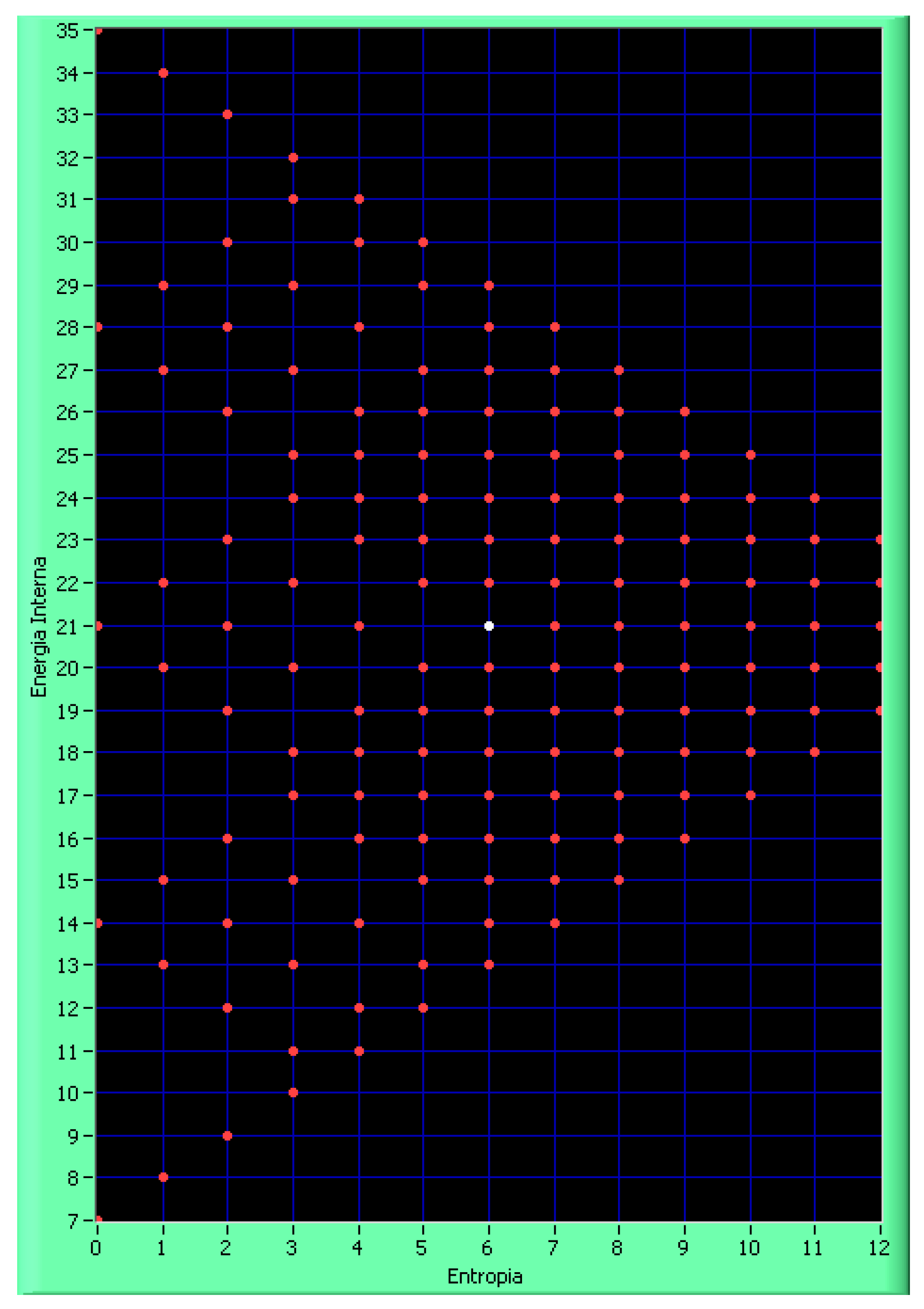
with k being the length of the sequence of elements, and k₁, k₂, …, k_r representing the number of times that the first, second, …, r-th element repeats, respectively. The sum of the states reported in the previous table yields a partition of the set of states, which is 5⁷ = 78,125. Figure 2 shows the table of sub-scenarios in the ES plane. In gray, it displays the 13 levels of entropy within the allowable range of 0–12 and the 29 levels of energy within the allowable range of 7–35. Additionally, for brevity, the boxes indicate the sub-scenarios S7_# with only the last number #. Finally, we have divided the flat occupancy surface into nine areas as follows:

I.

Low entropy, low energy (blue color);

II.

Low entropy, medium energy (light-blue color);

III.

Low entropy, high energy (green color);

IV.

Medium entropy, low energy (lilac color);

V.

Medium entropy, medium energy (white color);

VI.

Medium entropy, high energy (pink color);

VII.

High entropy, low energy (yellow color);

VIII.

High entropy, medium energy (orange color);

IX.

High entropy, high energy (red color).

Figure 2. Allocation of the sub-scenarios S7_# (indicated with only #). Here the different colors represent different area of interest in terms of Entropy and Energy as written above.

Figure 2. Allocation of the sub-scenarios S7_# (indicated with only #). Here the different colors represent different area of interest in terms of Entropy and Energy as written above.

From an analytical standpoint, it is evident that the best state is represented by the green area, i.e., Area III, which corresponds to high energy and low entropy. This means that the system under consideration has a fast dynamic that does not create disorder. The two worst areas, for different reasons that we will describe, are Area VII (yellow) and Area IX (red). Area VII (yellow) describes states characterized by low energy and high entropy. This state is the worst if the goal is to bring the system back to a situation of greater equilibrium. In other words, it will be necessary to wait a long time to rebalance the system whose characteristic state falls into the yellow area. Area IX (red) describes states characterized by high energy and high entropy. These are systems characterized by high-speed dynamics close to chaos. The decision-maker will, therefore, have very short decision times, but if the decisions taken are correct, the system, given the high energy, can be rebalanced much more quickly than in the cases falling into Area VII. The last extreme area is Area I (blue), characterized by low energy and low entropy. Since energy is low, the systems represented by states included in the scenarios falling into this area will have very slow dynamics that do not create disorder, as the entropy is very low. In addition to these more extreme areas, we must also consider areas representing more hybrid scenarios. These areas are Area II (light blue), Area IV (lilac), Area VI (pink), and Area VIII (orange). Of these four hybrid areas, the best ones are II and VI, where entropy always has lower average values than energy. Less advantageous are the scenarios and states falling into Areas IV and VIII, where entropy is more significant than the system’s energy. In particular, Area VIII, except for VII and IX, is the worst of all. Finally, state V (white) is characterized by a complete balance between entropy and energy, with both assuming average values. As we will see later, Areas VII and IX are areas not occupied by admissible states, i.e., states in which the CSFs assume values on a scale of 1–5. Area VII represents low-energy chaos, while IX represents high-energy chaos. Figure 3 shows the table of the sub-scenarios S7_# indicated only by # in the SE plane, i.e., with varying energy and entropy. As you can see, for a given pair (S, E), there can correspond one or more sub-scenarios.

From Figure 2, it is evident that some macroscopic states characterized by the pairs (S, E) are not admissible and have been indicated in gray. Specifically, Areas VII and IX do not contain admissible states within them and are, therefore, to be considered as states already out of control because they are chaotic. In relation to the previous figure, in Figure 3 below, we report the level of degeneracy of different ordered pairs (E, S), from which it can be seen that the most degenerate levels occur in the central area of the figure, Area V (white), followed by Areas IV and VI, then II and VII, and finally by VII, IX, III, and I. By the level of degeneracy, we mean the presence of multiple sub-scenarios for the same pair (S, E).

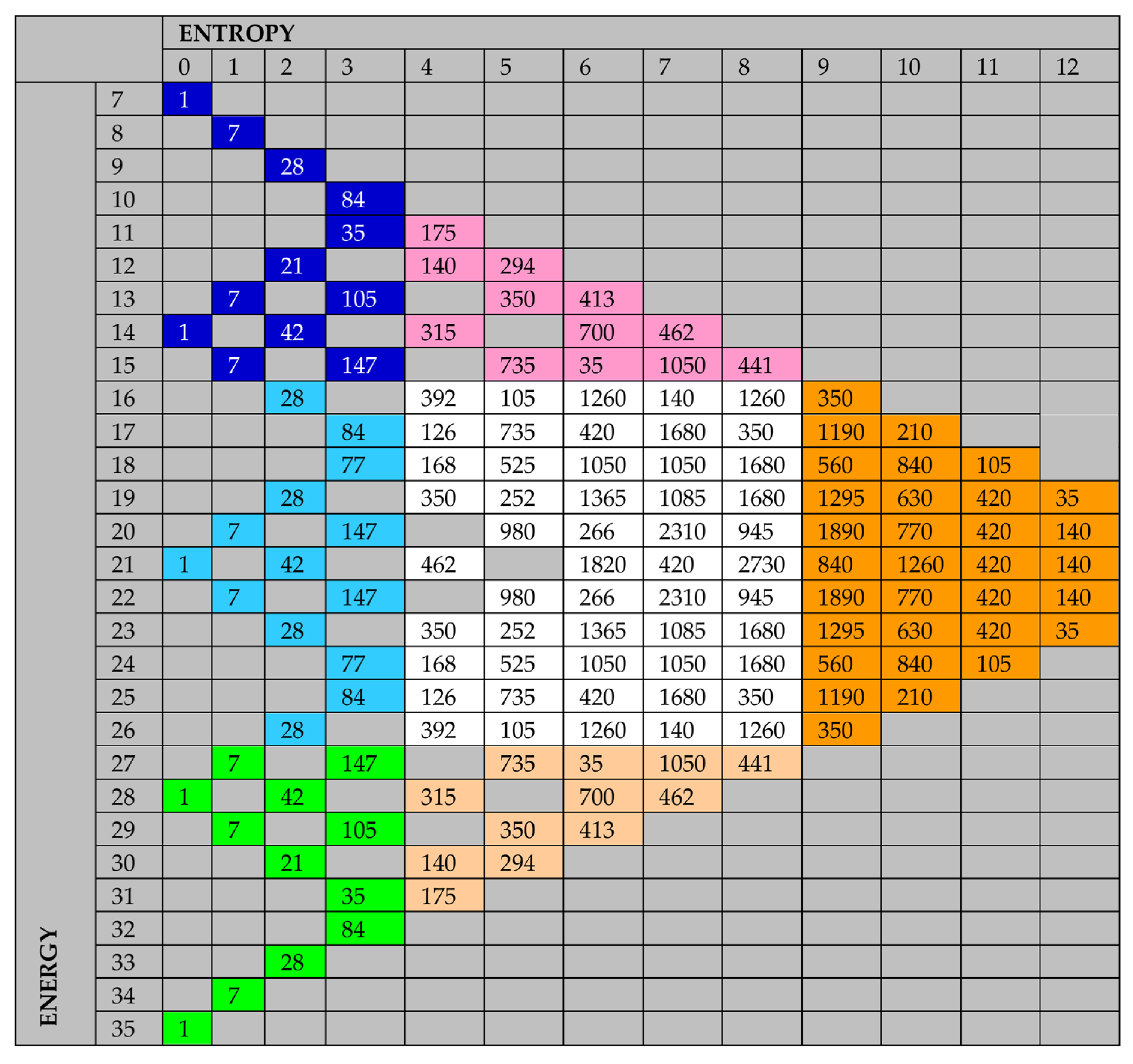
Figure 4 shows the table of the number of microscopic states, represented by a seven-component n-tuple, corresponding to the same macroscopic state represented by the pair (S, E).

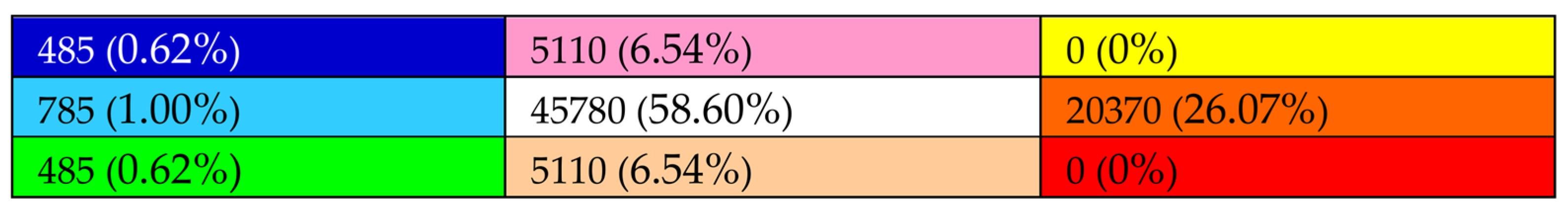
Finally, Figure 5 represents the number of states for each area and their % for a total of 78,125 states.

4.2. S6 Scenario

As previously mentioned in the preceding section, the modelled systems, as in reality, can exhibit different dynamics depending on other parameters such as space or time. Therefore, it may be that all CSFs vary simultaneously (general case referred to as S7) or that only some of them have gradients, while the remaining ones remain in their previously evaluated states. Furthermore, one might consider the possibility of creating the appropriate conditions for a forced transition from one state to another, needing or wanting to keep some pointers fixed while allowing others to vary. In such cases, it becomes interesting to also consider scenarios from S6 to S0.

The study of scenario S6 is obtained from S7 by reducing the state space by one dimension.

The total number of sub-scenarios is 84. This value is calculated using the well-known expression from combinatorial mathematics for calculating combinations with repetition of n = 4 distinct elements taken k = 6 at a time, which is applicable in the current case

$$C_{5,6}=\left(\begin{array}{c}4+6-1\\ 6\end{array}\right)=\frac{9!}{6!3!}=84.$$

(18)

In other words, having a fixed parameter, from a mathematical standpoint, is expressed by reducing the set of elements to choose from by one unit. This means going from the five elements {1,2,3,4,5} to the remaining four, by excluding the fixed one and decreasing the sequence length by one unit, changing from seven to six. Similar to S7, this scenario can also be deconstructed into sub-scenarios containing the same elements except for permutations. In detail, scenario S6 breaks down into the following nine sub-scenarios, taking into consideration their characterization.

Table 3. S6 sub-scenarios, where the symbol ◊ indicates the composition of the micro-state string as described above.

Sub-Scenario	Characterization	N.Sub-Scenarios	N.States
S6_1	6	4	4 × (6!/6!) = 4
S6_2	5◊1	12	12 × (6!/5!) = 72
S6_3	4◊2	12	12 × (6!/4!2!) = 180
S6_4	4◊1◊1	12	12 × (6!/4!) = 360
S6_5	3◊3	6	6 × (6!/3!3!) = 120
S6_6	3◊2◊1	24	24 × (6!/3!2!) = 1440
S6_7	3◊1◊1◊1	4	4 × (6!/3!) = 480
S6_8	2◊2◊2	4	4 × (6!/2!2!2!) = 360
S6_9	2◊2◊1◊1	6	6 × (6!/2!2!) = 1080

shows the number of sub-scenarios and states. However, entropy and energy calculations will not be performed in these cases since the information is incomplete. In other words, the information about which CSF is considered fixed is not known in advance. Additionally, if one wishes to calculate energies and entropies, it would be more interesting to calculate those related to the system’s rebalancing. Nevertheless, this is beyond the scope of this section, as it falls under the realm of management strategies for the implementation of an advanced DSS.

By summing up the states, it is found that the total is 4096, which coincides with the expected theoretical value of 4⁶, exactly equal to the number of combinations of four elements taken six at a time (since the seventh element was fixed). However, the previous table possesses greater expressive power, as it subdivides the S6 scenario into sub-scenarios, deconstructing the information.

4.3. S5 Scenario

The study of the S5 scenario is obtained from S7 by reducing the number of dimensions by two or using S6 by reducing the number of dimensions by one. The total number of sub-scenarios is equal to 56. This value is calculated through combinations with the repetition of n = 4 distinct elements taken k = 5 at a time, i.e., assuming that of the seven pointers two are fixed and equal; therefore, in the case under study we find

$$C_{4,5}=\left(\begin{array}{c}4+5-1\\ 5\end{array}\right)=\frac{8!}{5!3!}=56.$$

(19)

In other words, having a fixed parameter from a mathematical point of view is expressed by reducing the set of elements to choose from by one unit, so going from the five elements {1,2,3,4,5} to four by discarding the fixed one and decreasing the length of the sequence by two units, i.e., from seven to five. From a purely statistical point of view, we could also consider the case n = 3 and k = 5, which corresponds to fixing two CSFs with different values, but this is not of interest in the present analysis, as it would ultimately result in reconstructing, or re-structuring, the space of events back to 5⁷. Instead, we are specifically interested in the case where a sequence has two fixed CSFs which take on specific values while the others are different. Just like S7 and S6, this scenario can also be deconstructed into sub-scenarios containing the same elements except for permutations. In detail, scenario S5 deconstructs into the following six sub-scenarios based on characterization.

Table 4. S5 sub-scenarios, where the symbol ◊ indicates the composition of the micro-state string as described above.

Sub-Scenario	Characterization	N.Sub-Scenarios	N.States
S5_1	5	4	4 × (5!/5!) = 4
S5_2	4◊1	12	12 × (5!/4!) = 60
S5_3	3◊2	12	12 × (5!/3!2!) = 120
S5_4	3◊1◊1	12	12 × (5!/3!) = 240
S5_5	2◊2◊1	12	12 × (5!/2!2!) = 360
S5_6	2◊1◊1◊1	4	4 × (5!/2!) = 240

shows the number of sub-scenarios and states. Unlike S7 and similar to S6, entropies and energies will not be calculated in these cases since the information is incomplete.

By summing the states, it is found that their total number is 1024, which coincides with the expected theoretical value of 4⁵, precisely the number of combinations of four elements taken five at a time (since two CSFs have been fixed to the same value). The previous table possesses greater expressive power as it subdivides scenario S5 into sub-scenarios, thereby deconstructing the information.

4.4. S4 Scenario

The study of scenario S4 is obtained from S7 by reducing the number of dimensions by three. The total number of sub-scenarios is 35. This value is calculated using combinations with repetition of n = 4 distinct elements taken k = 4 at a time:

$$C_{4,4}=\left(\begin{array}{c}4+4-1\\ 4\end{array}\right)=\frac{7!}{4!3!}=35.$$

(20)

In other words, fixing a parameter from a mathematical point of view is expressed by reducing the set of elements to be chosen by one unit. This means going from the set of five {1, 2, 3, 4, 5} to the set of four obtained by discarding the fixed element and decreasing the length of the sequence by three units, i.e., going from seven to four. Like in the previous cases, scenario S4 can be deconstructed into sub-scenarios containing the same elements with permutations. In detail, scenario S4 deconstructs into the following five sub-scenarios, taking into account characterization:

Table 5. S4 sub-scenarios, where the symbol ◊ was described above.

Sub-Scenario	Characterization	N.Sub-Scenarios	N.States
S4_1	4	4	4 × (4!/4!) = 4
S4_2	3◊1	12	12 × (4!/3!) = 48
S4_3	2◊2	6	6 × (4!/2!2!) = 36
S4_4	2◊1◊1	12	12 × (4!/2!) = 144
S4_5	1◊1◊1◊1	1	1 × (4!) = 24

shows the number of sub-scenarios and states. Similar to S6, S5, and S6, entropies and energies will not be calculated for S4.

Summing the states reveals that their total number is 256, which coincides with the expected theoretical value of 4⁴, precisely the number of combinations of four elements taken four at a time (since three pointers have been fixed to the same value). The previous table possesses greater expressive power, as it subdivides scenario S4 into sub-scenarios, thereby deconstructing the information.

4.5. S3 Scenario

The study of scenario S3 is obtained from S7 by reducing the number of dimensions by four. The total number of sub-scenarios is 20. This value is calculated using combinations with repetitions of n = 4 distinct elements taken k = 3 at a time

$$C_{4,3}=\left(\begin{array}{c}4+3-1\\ 3\end{array}\right)=\frac{6!}{3!3!}=20.$$

(21)

In other words, fixing a parameter from a mathematical point of view is expressed by reducing the set of elements to be chosen by one unit. This means going from the set of five {1,2,3,4,5} to the set of four obtained by discarding the fixed element and decreasing the length of the sequence by four units, i.e., going from seven to three. Like in the previous cases, scenario S3 can be deconstructed into sub-scenarios containing the same elements with permutations. In detail, scenario S3 deconstructs into the following three sub-scenarios, taking into account the characterization:

Table 6. S3 sub-scenarios, where the symbol ◊ was described above.

Sub-Scenario	Characterization	N.Sub-Scenarios	N.States
S3_1	3	4	4 × (3!/3!) = 4
S3_2	2◊1	12	12 × (3!/2!) = 36
S3_3	1◊1◊1	4	4 × (3!) = 24

shows the number of sub-scenarios and states. Similar to S6, S5, S4, and S6, entropies and energies will not be calculated for S3.

Summing the states reveals that their total number is 64, which coincides with the expected theoretical value of 43, precisely the number of combinations of four elements taken three at a time (since four pointers have been fixed to the same value). The previous table possesses greater expressive power as it subdivides scenario S3 into sub-scenarios, thereby deconstructing the information.

4.6. S2, S1, and S0 Scenarios

The study of scenario S2 is obtained from S7 by reducing the number of dimensions by five. The total number of sub-scenarios is 10. This value is calculated using combinations with repetition of n = 4 distinct elements taken k = 2 at a time. In other words, fixing a parameter from a mathematical point of view is expressed by reducing the set of elements to be chosen by one unit. This means going from the set of seven elements to six, with one element fixed:

$$C_{4,2}=\left(\begin{array}{c}4+2-1\\ 2\end{array}\right)=\frac{5!}{2!3!}=10$$

(22)

The scenario S2 deconstructs into the following two sub-scenarios, taking into account the characterization:

Here, in

Table 7. S2 sub-scenarios, where the symbol ◊ was described above.

Sub-Scenario	Characterization	N.Sub-Scenarios	N.States
S2_1	2	4	4 × (2!/2!) = 4
S2_2	1◊1	6	6 × (2!) = 12

, there are the following possibilities.

Summing the states reveals that their total number is 16, which coincides with the expected theoretical value of 4², precisely the number of combinations of four elements taken two at a time (since five pointers have been fixed to the same value). The previous table possesses greater expressive power, as it subdivides scenario S2 into sub-scenarios, thereby deconstructing the information. The study of scenario S1 is obtained from S7 by reducing the number of dimensions by six. It has a single sub-scenario given using the variability of a single element chosen from four possibilities. Therefore, there will be four states in total. The scenario with no variable elements, or equivalently with seven fixed elements, coincides with its single sub-scenario, and its single element consists of a sequence with seven equal pointers. The only possible state is, of course, theoretically expected as 4⁰.

4.7. Considerations on Scenarios and States

As a final note on scenario classification, it should be mentioned that for scenarios S6–S0, we considered the fixed CSFs not only to be equal, but we also treated them as a monolithic block. This means that they cannot mix with the other CSFs in the sequence; otherwise, the number of states would significantly increase. The analysis of scenarios S6–S0 demonstrate not only the obvious fact that the more fixed CSFs we have, the fewer possibilities there are to bring the system back to equilibrium, but it also shows the different ways in which it can be carried out. In other words, we have determined the various sub-scenarios. To discuss the equilibrium of a system, unfortunately, the current representation or classification into scenario families is not effective, just as it is inadequate for trend analysis and forecasting. For these reasons, in the following section, we will adopt a more advanced representation suitable for achieving the stated aim.

5. Scenarios and States: Representation and Characterization for Decision Path Making

In this section, instead of adopting a statistical classification of scenarios into sub-scenarios, a more advanced analytical technique will be employed, which enables a more suitable clustering for the study of the evolutionary dynamics of a system represented using the seven introduced CSFs. The nearly eighty-thousand (specifically, 78,125) cases are categorized into 12 classes of fundamental scenarios, defined as follows:

• FEE—fundamental equilibrium scenarios;
• FES—fundamental explosive scenarios;
• FIS—fundamental implosive scenarios;
• FAS—fundamental alterations scenarios;
• FBIS—fundamental bipolar imbalance scenarios;
• FMIS—fundamental multiphasic imbalance scenarios;
• EMDS—explosive multi-weighted dominance scenarios;
• IMDS—implosive multi-weighted dominance scenarios;
• LEMDS—low-energy multi-weighted dominance scenarios;
• MEMDS—medium-energy multi-weighted dominance scenarios with trend;
• HEMDS—high-energy multi-weighted dominance scenarios;
• HES—high-entropy scenarios.

5.1. FEE—Fundamental Equilibrium Scenarios

In the following section, we describe five equilibrium scenarios.

Scenario N = 1 represents a situation of neutral equilibrium among the optimal equilibria; it is the medium-energy equilibrium scenario, characterized by CSFs which, while having their dynamics, do not produce significant alterations. In this sub-scenario, E = 21, and S = 0.

Scenario N = 2 is a low-energy equilibrium, meaning that the system has slow dynamics. In this sub-scenario, E = 14, and S = 0.

Scenario N = 3 corresponds to the frozen scenario, meaning the system has almost no dynamics. It is substantially different from N = 1, where there are some dynamics but is still at equilibrium. In this case, there are extremely slow dynamics, as if the scenario were frozen. Therefore, if there were alterations, they would be very slow or of a transient nature. In this sub-scenario, E = 7, and S = 0.

Scenario N = 4 corresponds to a significantly energetic scenario, which can become unstable because small fluctuations can lead to alterations or imbalances. In this sub-scenario, E = 28, and S = 0.

Scenario N = 5 corresponds to an equilibrium scenario, but at very high energy; therefore, small unbalanced oscillations can lead to chaos. In this sub-scenario, E = 35, and S = 0.

The five FEE sub-scenarios have the characteristics of having E ∊ [7, 35] and S = 0, from which it can be seen that they fall into Areas I (blue), II (light blue), and III (green). In the DSS (decision support system) model, just like in chaos and complexity theory, the FEE represent five fundamental attractors. The maximum equilibrium attractor is FEE_5, while the minimum is FEE_3. We could add the lower and upper extremes as well. The lower one would represent the beginning of the hibernation space, and the upper one the chaos. In that case, we would have seven attractors, and a match could be created between the proposed model and René Thom’s catastrophe theory. In mathematical terms, a catastrophe is a degenerate (or non-regular) critical point of a smooth (everywhere differentiable) surface defined in an n-dimensional Euclidean space, as these points correspond to radical bifurcations in the system’s behavior.

5.2. FES—Fundamental Explosive Scenarios

In the following, we describe seven explosive scenarios.

For each i of them, X_i take, respectively, the value five, while the other indexes X_j of 7-tupla take an integer value a_i such that 2 ≤ X_j ≤ 4.

The seven FES scenarios are strongly unstable scenarios for at least one of the systemic components (corresponding to the explosive characteristic CSF with a value of five).

The seven FES sub-scenarios have the characteristics of having E ∊ [23, 29] and S ∊ [1, 7], which means they fall into Areas II (light blue), III (green), V (black and white), and VI (pink).

5.3. FIS—Fundamental Implosive Scenarios

In the following, we describe seven implosive scenarios.

For each i of them, X_i take, respectively, the value one, while the other indexes X_j of 7-tupla take an integer value a_i such that 2 ≤ X_j ≤ 4.

The seven FIS scenarios are dominated by the systemic components b_i, even though there is an implosion of at least one characteristic CSF (corresponding to the implosive characteristic CSF with a value of one).

The seven FIS sub-scenarios have the characteristic of having E ∊ [13, 25] and S ∊ [1, 7], which means they fall into Areas I (blue), II (light blue), IV (purple), and V (white).

5.4. FIS—Fundamental Alteration Scenarios

In the following, we describe seven scenarios with specific alterations.

Case N. 20 is characterized as follows:

$$\exists \mathit{i}\in \left\{\mathbf{1},\mathbf{2},\mathbf{3},\mathbf{4},\mathbf{5},\mathbf{6},\mathbf{7}\right\}:{\mathit{X}}_{\mathit{i}}\ne \mathbf{3},{\mathit{X}}_{\mathit{i}}=\mathbf{2},{\mathit{X}}_{\mathit{j}}=\mathbf{3} \mathit{with} \mathit{j}\ne \mathit{i}$$

Case N. 21 is characterized as follows:

$$\exists \mathit{i}\in \left\{\mathbf{1},\mathbf{2},\mathbf{3},\mathbf{4},\mathbf{5},\mathbf{6},\mathbf{7}\right\}\mathit{:}{\mathit{X}}_{\mathit{i}}\ne \mathbf{3},{\mathit{X}}_{\mathit{i}}=\mathbf{4},{\mathit{X}}_{\mathit{j}}=\mathbf{3} \mathit{w}\mathit{i}\mathit{t}\mathit{h} \mathit{j}\ne \mathit{i}$$

Case N. 22 is characterized as follows:

$$\exists \mathit{i},\mathit{k}\in \left\{\mathbf{1},\mathbf{2},\mathbf{3},\mathbf{4},\mathbf{5},\mathbf{6},\mathbf{7}\right\}:{\mathit{X}}_{\mathit{i}}\ne \mathbf{3},{\mathit{X}}_{\mathit{i}}=\mathbf{2},{\mathit{X}}_{\mathit{k}}\ne \mathbf{3},{\mathit{X}}_{\mathit{k}}=\mathbf{2},{\mathit{X}}_{\mathit{j}}=\mathbf{3} \mathit{w}\mathit{i}\mathit{t}\mathit{h} \mathit{j}\ne \mathit{i},\mathit{k}$$

Case N. 23 is characterized as follows:

$$\exists \mathit{i},\mathit{k}\in \left\{\mathbf{1},\mathbf{2},\mathbf{3},\mathbf{4},\mathbf{5},\mathbf{6},\mathbf{7}\right\}:{\mathit{X}}_{\mathit{i}}\ne \mathbf{3},{\mathit{X}}_{\mathit{i}}=\mathbf{4},{\mathit{X}}_{\mathit{k}}\ne \mathbf{3},{\mathit{X}}_{\mathit{k}}=\mathbf{4},{\mathit{X}}_{\mathit{j}}=\mathbf{3} \mathit{w}\mathit{i}\mathit{t}\mathit{h} \mathit{j}\ne \mathit{i},\mathit{k}$$

Case N. 24 is characterized as follows:

$$\exists \mathit{i},\mathit{k}\in \left\{\mathbf{1},\mathbf{2},\mathbf{3},\mathbf{4},\mathbf{5},\mathbf{6},\mathbf{7}\right\}:{\mathit{X}}_{\mathit{i}}\ne \mathbf{3},{\mathit{X}}_{\mathit{i}}=\mathbf{2},{\mathit{X}}_{\mathit{k}}\ne \mathbf{3},{\mathit{X}}_{\mathit{k}}=\mathbf{4},{\mathit{X}}_{\mathit{j}}=\mathbf{3} \mathit{w}\mathit{i}\mathit{t}\mathit{h} \mathit{j}\ne \mathit{i},\mathit{k}$$

Case N. 25 is characterized as follows:

$$\exists \mathit{t}\mathit{h}\mathit{r}\mathit{e}\mathit{e} \mathit{p}\mathit{o}\mathit{i}\mathit{n}\mathit{t}\mathit{e}\mathit{r}\mathit{s} \mathit{i},\mathit{k},\mathit{r}\in \left\{\mathbf{1},\mathbf{2},\mathbf{3},\mathbf{4},\mathbf{5},\mathbf{6},\mathbf{7}\right\}:{\mathit{X}}_{\mathit{i}}={\mathit{X}}_{\mathit{k}}={\mathit{X}}_{\mathit{r}}\ne \mathbf{3},{\mathit{X}}_{\mathit{i}}={\mathit{X}}_{\mathit{k}}={\mathit{X}}_{\mathit{r}}=\mathbf{2},{\mathit{X}}_{\mathit{j}}=\mathbf{3} \mathit{w}\mathit{i}\mathit{t}\mathit{h} \mathit{j}\ne \mathit{i},\mathit{k},\mathit{r}$$

Case N. 26 is characterized as follows:

$$\exists \mathit{t}\mathit{h}\mathit{r}\mathit{e}\mathit{e} \mathit{p}\mathit{o}\mathit{i}\mathit{n}\mathit{t}\mathit{e}\mathit{r}\mathit{s} \mathit{i},\mathit{k},\mathit{r}\in \left\{\mathbf{1},\mathit{2},\mathbf{3},\mathbf{4},\mathbf{5},\mathbf{6},\mathbf{7}\right\}:{\mathit{X}}_{\mathit{i}}={\mathit{X}}_{\mathit{k}}={\mathit{X}}_{\mathit{r}}\ne \mathbf{3},{\mathit{X}}_{\mathit{i}}={\mathit{X}}_{\mathit{k}}={\mathit{X}}_{\mathit{r}}=\mathbf{4},{\mathit{X}}_{\mathit{j}}=\mathbf{3} \mathit{w}\mathit{i}\mathit{t}\mathit{h} \mathit{j}\ne \mathit{i},\mathit{k},\mathit{r}$$

The FAS scenarios are scenarios dominated by the value three; they indicate situations of primary non-equilibrium, meaning alterations which normally indicate a departure from a state of equilibrium. These are situations where the intervention of the decision-maker to restore the system to normalcy is desirable. In such situations, the successful outcome of the rebalancing action will be short or moderately short and effective.

The seven FAS sub-scenarios are characterized by having E ∊ [18, 24] and S ∊ [1, 3], from which it can be seen that they all fall within Area II (light blue).

The names of the FAS sub-scenarios highlight the presence of additional variability indicated using the term “Phase” (biphasic, triphasic, etc.); this variable expresses the number of different values that the CSFs can take on; therefore, “biphasic” means that all CSFs assume two possible values, “triphasic” means three values, and so on.

5.5. FBIS—Fundamental Bipolar Imbalance Scenarios

In the following, we describe three scenarios with specific imbalance.

Here, the coefficients X_i are defined as follows case by case.

Case N. 27 is characterized as follows:

$$\mathit{\exists }\mathit{i},\mathit{k}\mathit{\in }\left\{\mathbf{1},\mathbf{2},\mathbf{3},\mathbf{4},\mathbf{5},\mathbf{6},\mathbf{7}\right\}\mathit{:}{\mathit{X}}_{\mathit{i}}\mathit{=}\mathbf{1}, {\mathit{X}}_{\mathit{k}}\mathit{=}\mathbf{5}, \mathbf{2}\mathit{\le }{\mathit{X}}_{\mathit{j}}\mathit{\le }\mathbf{4} \mathit{w}\mathit{i}\mathit{t}\mathit{h} \mathit{j}\mathit{\ne }\mathit{i},\mathit{k} \mathit{a}\mathit{n}\mathit{d} {\displaystyle \mathbf{\sum }}_{\mathit{j}\mathit{=}\mathbf{1}}^{\mathbf{5}}{\mathit{X}}_{\mathit{j}}\mathit{>}\mathbf{15}$$

with E ∊ [22, 26] and S ∊ [4, 8].

Case N. 28 is characterized as follows:

$$\mathit{\exists }\mathit{i},\mathit{k}\mathit{\in }\left\{\mathbf{1},\mathbf{2},\mathbf{3},\mathbf{4},\mathbf{5},\mathbf{6},\mathbf{7}\right\}\mathit{:}{\mathit{X}}_{\mathit{i}}\mathit{=}\mathbf{1}, {\mathit{X}}_{\mathit{k}}\mathit{=}\mathbf{5}, \mathbf{2}\mathit{\le }{\mathit{X}}_{\mathit{j}}\mathit{\le }\mathbf{4} \mathit{w}\mathit{i}\mathit{t}\mathit{h} \mathit{j}\mathit{\ne }\mathit{i},\mathit{k} \mathit{a}\mathit{n}\mathit{d} {\displaystyle \mathbf{\sum }}_{\mathit{j}\mathit{=}\mathbf{1}}^{\mathbf{5}}{\mathit{X}}_{\mathit{j}}\mathit{<}\mathbf{15}$$

with E ∊ [16, 20] and S ∊ [4, 8].

Case N. 29 is characterized as follows:

$$\mathit{\exists }\mathit{i},\mathit{k}\mathit{\in }\left\{\mathbf{1},\mathbf{2},\mathbf{3},\mathbf{4},\mathbf{5},\mathbf{6},\mathbf{7}\right\}:{\mathit{X}}_{\mathit{i}}\mathit{=}\mathbf{1}, {\mathit{X}}_{\mathit{k}}\mathit{=}\mathbf{5}, \mathbf{2}\mathit{\le }{\mathit{X}}_{\mathit{j}}\mathit{\le }\mathbf{4} \mathit{w}\mathit{i}\mathit{t}\mathit{h} \mathit{j}\mathit{\ne }\mathit{i},\mathit{k} \mathit{a}\mathit{n}\mathit{d} {\displaystyle \mathbf{\sum }}_{\mathit{j}\mathit{=}\mathbf{1}}^{\mathbf{5}}{\mathit{X}}_{\mathit{j}}\mathit{=}\mathbf{15}$$

with E = 21 and S = 4, 6, 8.

It is easy to verify that, in the case of FBIS sub-scenarios, E ∊ [16, 26] and S ∊ [4, 8], from which it can be seen that they all fall within Area V (white).

5.6. FMIS—Fundamental Multiphasic Imbalance Scenarios

Also, here, we describe three scenarios with specific imbalance.

Here, the coefficients X_i are defined as follows case by case.

Case N. 30 is characterized as follows:

$$\exists \mathit{i},\mathit{k},\mathit{r},\mathit{s},\mathit{t}\in \left\{\mathbf{1},\mathbf{2},\mathbf{3},\mathbf{4},\mathbf{5},\mathbf{6},\mathbf{7}\right\}:{\mathit{X}}_{\mathit{i}}=\mathbf{1}, {\mathit{X}}_{\mathit{k}}=\mathbf{2}, {\mathit{X}}_{\mathit{r}}=\mathbf{3}, {\mathit{X}}_{\mathit{s}}=\mathbf{4}, {\mathit{X}}_{\mathit{t}}=\mathbf{5}, \mathit{a}\mathit{n}\mathit{d} {\displaystyle \mathbf{\sum }}_{\mathit{j}=\mathbf{1}}^{\mathbf{2}}{\mathit{X}}_{\mathit{j}}>\mathbf{6}$$

with E ∊ [22, 25] and S ∊ [7, 9].

Case N. 31 is characterized as follows:

$$\exists \mathit{i},\mathit{k},\mathit{r},\mathit{s},\mathit{t}\in \left\{\mathbf{1},\mathbf{2},\mathbf{3},\mathbf{4},\mathbf{5},\mathbf{6},\mathbf{7}\right\}:{\mathit{X}}_{\mathit{i}}=\mathbf{1}, {\mathit{X}}_{\mathit{k}}=\mathbf{2}, {\mathit{X}}_{\mathit{r}}=\mathbf{3}, {\mathit{X}}_{\mathit{s}}=\mathbf{4}, {\mathit{X}}_{\mathit{t}}=\mathbf{5}, \mathit{a}\mathit{n}\mathit{d} {\displaystyle \mathbf{\sum }}_{\mathit{j}=\mathbf{1}}^{\mathbf{2}}{\mathit{X}}_{\mathit{j}}<\mathbf{6}$$

with E ∊ [17, 20] and S ∊ [7, 9].

Case N. 32 is characterized as follows:

$$\exists \mathit{i},\mathit{k},\mathit{r},\mathit{s},\mathit{t}\in \left\{\mathbf{1},\mathbf{2},\mathbf{3},\mathbf{4},\mathbf{5},\mathbf{6},\mathbf{7}\right\}:{\mathit{X}}_{\mathit{i}}=\mathbf{1}, {\mathit{X}}_{\mathit{k}}=\mathbf{2}, {\mathit{X}}_{\mathit{r}}=\mathbf{3}, {\mathit{X}}_{\mathit{s}}=\mathbf{4}, {\mathit{X}}_{\mathit{t}}=\mathbf{5}, \mathit{a}\mathit{n}\mathit{d} {\displaystyle \mathbf{\sum }}_{\mathit{j}=\mathbf{1}}^{\mathbf{2}}{\mathit{X}}_{\mathit{j}}=\mathbf{6}$$

with E = 21 and S ∊ [6, 10].

Combining the three previous sub-scenarios, it is easy to verify that in the case of FMIS scenarios, E ∊ [17, 25] and S ∊ [6, 10], from which it can be seen that they fall within Area V (white) and VIII (orange).

5.7. MEDS—Multi-Weighted Explosive Dominance Scenarios

Here, we describe five scenarios with specific explosive dominance.

The coefficients X_i are defined as follows case by case.

Case N. 33 is characterized as follows:

$$\exists \mathit{i},\mathit{k}\in \left\{\mathbf{1},\mathbf{2},\mathbf{3},\mathbf{4},\mathbf{5},\mathbf{6},\mathbf{7}\right\}:{\mathit{X}}_{\mathit{i}}={\mathit{X}}_{\mathit{k}}=\mathbf{5}, \mathbf{2}\le {\mathit{X}}_{\mathit{j}}\le \mathbf{4} \mathit{w}\mathit{i}\mathit{t}\mathit{h} \mathit{j}\ne \mathit{i},\mathit{k}$$

with E ∊ [20, 30] and S ∊ [2, 8].

Case N. 34 is characterized as follows:

$$\exists \mathit{i},\mathit{k},\mathit{r}\in \left\{\mathbf{1},\mathbf{2},\mathbf{3},\mathbf{4},\mathbf{5},\mathbf{6},\mathbf{7}\right\}:{\mathit{X}}_{\mathit{i}}={\mathit{X}}_{\mathit{k}}={\mathit{X}}_{\mathit{r}}=\mathbf{5}, \mathbf{2}\le {\mathit{X}}_{\mathit{j}}\le \mathbf{4} \mathit{w}\mathit{i}\mathit{t}\mathit{h} \mathit{j}\ne \mathit{i},\mathit{k},\mathit{r}$$

with E ∊ [27, 31] and S ∊ [3, 9].

Case N. 35 is characterized as follows:

$$\exists \mathit{i},\mathit{k},\mathit{r},\mathit{s}\in \left\{\mathbf{1},\mathbf{2},\mathbf{3},\mathbf{4},\mathbf{5},\mathbf{6},\mathbf{7}\right\}:{\mathit{X}}_{\mathit{i}}={\mathit{X}}_{\mathit{k}}={\mathit{X}}_{\mathit{r}}={\mathit{X}}_{\mathit{s}}=\mathbf{5}, \mathbf{2}\le {\mathit{X}}_{\mathit{j}}\le \mathbf{4} \mathit{w}\mathit{i}\mathit{t}\mathit{h} \mathit{j}\ne \mathit{i},\mathit{k},\mathit{r},\mathit{s}$$

with E ∊ [26, 32] and S ∊ [3, 9].

Case N. 36 is characterized as follows:

$$\exists \mathit{i},\mathit{k},\mathit{r},\mathit{s},\mathit{t}\in \left\{\mathbf{1},\mathbf{2},\mathbf{3},\mathbf{4},\mathbf{5},\mathbf{6},\mathbf{7}\right\}:{\mathit{X}}_{\mathit{i}}={\mathit{X}}_{\mathit{k}}={\mathit{X}}_{\mathit{r}}={\mathit{X}}_{\mathit{s}}={\mathit{X}}_{\mathit{t}}=\mathbf{5}, \mathbf{2}\le {\mathit{X}}_{\mathit{j}}\le \mathbf{4} \mathit{w}\mathit{i}\mathit{t}\mathit{h} \mathit{j}\ne \mathit{i},\mathit{k},\mathit{r},\mathit{s},\mathit{t}$$

with E ∊ [29, 33] and S ∊ [2, 6].

Case N. 37 is characterized as follows:

$$\begin{gathered} \exists \mathit{i},\mathit{k},\mathit{r},\mathit{s},\mathit{t},\mathit{u}\in \left\{\mathbf{1},\mathbf{2},\mathbf{3},\mathbf{4},\mathbf{5},\mathbf{6},\mathbf{7}\right\}:{\mathit{X}}_{\mathit{i}}={\mathit{X}}_{\mathit{k}}={\mathit{X}}_{\mathit{r}}={\mathit{X}}_{\mathit{s}}={\mathit{X}}_{\mathit{t}}={\mathit{X}}_{\mathit{u}}=\mathbf{5}, \mathbf{2}\le {\mathit{X}}_{\mathit{j}}\le \mathbf{4} \\ \mathit{w}\mathit{i}\mathit{t}\mathit{h} \mathit{j}\ne \mathit{i},\mathit{k},\mathit{r},\mathit{s},\mathit{t},\mathit{u} \end{gathered}$$

with E ∊ [32, 34] and S ∊ [1, 3].

Combining the five previous sub-scenarios, it is easy to verify that in the case of MEDS scenarios, E ∊ [20, 34] and S ∊ v[1, 9], from which it can be seen that they fall within Area II (blue), III (green), V (white), VI (pink), and VIII (orange).

5.8. MIDS—Multi-Weighted Implosive Dominance Scenarios

Here, we describe five scenarios with specific implosive dominance.

The coefficients X_i are defined as follows case by case.

Case N. 38 is characterized as follows:

$$\exists \mathit{i},\mathit{k}\in \left\{\mathbf{1},\mathbf{2},\mathbf{3},\mathbf{4},\mathbf{5},\mathbf{6},\mathbf{7}\right\}:{\mathit{X}}_{\mathit{i}}={\mathit{X}}_{\mathit{k}}=\mathbf{1}, \mathbf{2}\le {\mathit{X}}_{\mathit{j}}\le \mathbf{4} \mathit{w}\mathit{i}\mathit{t}\mathit{h} \mathit{j}\ne \mathit{i},\mathit{k}$$

with E ∊ [12, 22] and S ∊ [2, 8].

Case N. 39 is characterized as follows:

$$\exists \mathit{i},\mathit{k},\mathit{r}\in \left\{\mathbf{1},\mathbf{2},\mathbf{3},\mathbf{4},\mathbf{5},\mathbf{6},\mathbf{7}\right\}:{\mathit{X}}_{\mathit{i}}={\mathit{X}}_{\mathit{k}}={\mathit{X}}_{\mathit{r}}=\mathbf{1}, \mathbf{2}\le {\mathit{X}}_{\mathit{j}}\le \mathbf{4} \mathit{w}\mathit{i}\mathit{t}\mathit{h} \mathit{j}\ne \mathit{i},\mathit{k},\mathit{r}$$

with E ∊ [11, 17] and S ∊ [3, 9].

Case N. 40 is characterized as follows:

$$\exists \mathit{i},\mathit{k},\mathit{r},\mathit{s}\in \left\{\mathbf{1},\mathbf{2},\mathbf{3},\mathbf{4},\mathbf{5},\mathbf{6},\mathbf{7}\right\}:{\mathit{X}}_{\mathit{i}}={\mathit{X}}_{\mathit{k}}={\mathit{X}}_{\mathit{r}}={\mathit{X}}_{\mathit{s}}=\mathbf{1}, \mathbf{2}\le {\mathit{X}}_{\mathit{j}}\le \mathbf{4} \mathit{w}\mathit{i}\mathit{t}\mathit{h} \mathit{j}\ne \mathit{i},\mathit{k},\mathit{r},\mathit{s}$$

with E ∊ [10, 16] and S ∊ [3, 9].

Case N. 41 is characterized as follows:

$$\exists \mathit{i},\mathit{k},\mathit{r},\mathit{s},\mathit{t}\in \left\{\mathbf{1},\mathbf{2},\mathbf{3},\mathbf{4},\mathbf{5},\mathbf{6},\mathbf{7}\right\}:{\mathit{X}}_{\mathit{i}}={\mathit{X}}_{\mathit{k}}={\mathit{X}}_{\mathit{r}}={\mathit{X}}_{\mathit{s}}={\mathit{X}}_{\mathit{t}}=\mathbf{1}, \mathbf{2}\le {\mathit{X}}_{\mathit{j}}\le \mathbf{4} \mathit{w}\mathit{i}\mathit{t}\mathit{h} \mathit{j}\ne \mathit{i},\mathit{k},\mathit{r},\mathit{s},\mathit{t}$$

with E ∊ [9, 13] and S ∊ [2, 6].

Case N. 42 is characterized as follows:

$$\begin{gathered} \exists \mathit{i},\mathit{k},\mathit{r},\mathit{s},\mathit{t},\mathit{u}\in \left\{\mathbf{1},\mathbf{2},\mathbf{3},\mathbf{4},\mathbf{5},\mathbf{6},\mathbf{7}\right\}:{\mathit{X}}_{\mathit{i}}={\mathit{X}}_{\mathit{k}}={\mathit{X}}_{\mathit{r}}={\mathit{X}}_{\mathit{s}}={\mathit{X}}_{\mathit{t}}={\mathit{X}}_{\mathit{u}}=\mathbf{1}, \mathbf{2}\le {\mathit{X}}_{\mathit{j}}\le \mathbf{4} \\ \mathit{w}\mathit{i}\mathit{t}\mathit{h} \mathit{j}\ne \mathit{i},\mathit{k},\mathit{r},\mathit{s},\mathit{t},\mathit{u} \end{gathered}$$

with E ∊ [8, 10] and S ∊ [1, 3].

Combining the five previous sub-scenarios, it is easy to verify that in the case of MIDS scenarios, E ∊ [8, 22] and S ∊ [1, 9], from which it can be seen that they fall within Area I (blue), II (celeste), IV (lilac), V (white), and VIII (orange).

5.9. MLEDS—Multi-Weighted Low Energy Dominance Scenarios

Here, we describe four scenarios with specifically low energy dominance.

The coefficients X_i are defined as follows case by case. It is important to state that the bimodal case is not considered because the system would be dominated by another energy level (i.e., medium or medium–high).

Case N. 43 is characterized as follows:

$$\exists \mathit{i},\mathit{k},\mathit{r}\in \left\{\mathbf{1},\mathbf{2},\mathbf{3},\mathbf{4},\mathbf{5},\mathbf{6},\mathbf{7}\right\}:{\mathit{X}}_{\mathit{i}}={\mathit{X}}_{\mathit{k}}={\mathit{X}}_{\mathit{r}}=\mathbf{2}, \mathbf{3}\le {\mathit{X}}_{\mathit{j}}\le \mathbf{4} \mathit{w}\mathit{i}\mathit{t}\mathit{h} \mathit{j}\ne \mathit{i},\mathit{k},\mathit{r}$$

with E ∊ [18, 22] and S ∊ [3, 6].

Case N. 44 is characterized as follows:

$$\exists \mathit{i},\mathit{k},\mathit{r},\mathit{s}\in \left\{\mathbf{1},\mathbf{2},\mathbf{3},\mathbf{4},\mathbf{5},\mathbf{6},\mathbf{7}\right\}:{\mathit{X}}_{\mathit{i}}={\mathit{X}}_{\mathit{k}}={\mathit{X}}_{\mathit{r}}={\mathit{X}}_{\mathit{s}}=\mathbf{2}, \mathbf{3}\le {\mathit{X}}_{\mathit{j}}\le \mathbf{4} \mathit{w}\mathit{i}\mathit{t}\mathit{h} \mathit{j}\ne \mathit{i},\mathit{k},\mathit{r},\mathit{s}$$

with E ∊ [17, 20] and S ∊ [3, 6].

Case N. 45 is characterized as follows:

$$\exists \mathit{i},\mathit{k},\mathit{r},\mathit{s},\mathit{t}\in \left\{\mathbf{1},\mathbf{2},\mathbf{3},\mathbf{4},\mathbf{5},\mathbf{6},\mathbf{7}\right\}:{\mathit{X}}_{\mathit{i}}={\mathit{X}}_{\mathit{k}}={\mathit{X}}_{\mathit{r}}={\mathit{X}}_{\mathit{s}}={\mathit{X}}_{\mathit{t}}=\mathbf{2}, \mathbf{3}\le {\mathit{X}}_{\mathit{j}}\le \mathbf{4} \mathit{w}\mathit{i}\mathit{t}\mathit{h} \mathit{j}\ne \mathit{i},\mathit{k},\mathit{r},\mathit{s},\mathit{t}$$

with E ∊ [16, 18] and S ∊ [2, 4].

Case N. 46 is characterized as follows:

$$\exists \mathit{i},\mathit{k},\mathit{r},\mathit{s},\mathit{t},\mathit{u}\in \left\{\mathbf{1},\mathbf{2},\mathbf{3},\mathbf{4},\mathbf{5},\mathbf{6},\mathbf{7}\right\}:{\mathit{X}}_{\mathit{i}}={\mathit{X}}_{\mathit{k}}={\mathit{X}}_{\mathit{r}}={\mathit{X}}_{\mathit{s}}={\mathit{X}}_{\mathit{t}}={\mathit{X}}_{\mathit{u}}=\mathbf{2}, \mathbf{3}\le {\mathit{X}}_{\mathit{j}}\le \mathbf{4} \mathit{w}\mathit{i}\mathit{t}\mathit{h} \mathit{j}\ne \mathit{i},\mathit{k},\mathit{r},\mathit{s},\mathit{t},\mathit{u}$$

with E ∊ [15, 16] and S ∊ [1, 2].

Combining the four previous sub-scenarios, it is easy to verify that in the case of MLEDS scenarios, E ∊ [15, 22] and S ∊ [1, 6], from which it can be seen that they fall within Area I (blue), II (light blue), IV (lilac), V (white), and VIII (orange).

5.10. MMEDS—Multi-Weighted Medium Energy Dominance Scenarios

Here, we describe twelve scenarios with specific medium energy dominance.

The coefficients X_i are defined as follows case by case. It is important to state that the bimodal case is not considered because the system would be dominated by another energy level (i.e., medium or medium–high).

Case N. 47 is characterized as follows:

$$\exists \mathit{i},\mathit{k},\mathit{r}\in \left\{\mathbf{1},\mathbf{2},\mathbf{3},\mathbf{4},\mathbf{5},\mathbf{6},\mathbf{7}\right\}:{\mathit{X}}_{\mathit{i}}={\mathit{X}}_{\mathit{k}}={\mathit{X}}_{\mathit{r}}=\mathbf{3}, {\mathit{X}}_{\mathit{j}\mathbf{1}}={\mathit{X}}_{\mathit{j}\mathbf{2}}={\mathit{X}}_{\mathit{j}\mathbf{3}}=\mathbf{4}, {\mathit{X}}_{\mathit{s}}=\mathbf{2} \mathit{w}\mathit{i}\mathit{t}\mathit{h} \mathit{j}\mathbf{1},\mathit{j}\mathbf{2},\mathit{j}\mathbf{3},\mathit{s}\ne \mathit{i},\mathit{k},\mathit{r}$$

with E = 23 and S = 4.

Case N. 48 is characterized as follows:

$$\exists \mathit{i},\mathit{k},\mathit{r},\mathit{s}\in \left\{\mathbf{1},\mathbf{2},\mathbf{3},\mathbf{4},\mathbf{5},\mathbf{6},\mathbf{7}\right\}:{\mathit{X}}_{\mathit{i}}={\mathit{X}}_{\mathit{k}}={\mathit{X}}_{\mathit{r}}={\mathit{X}}_{\mathit{s}}=\mathbf{3}, {\mathit{X}}_{\mathit{j}}=\mathbf{4} \mathit{w}\mathit{i}\mathit{t}\mathit{h} \mathit{j}\ne \mathit{i},\mathit{k},\mathit{r},\mathit{s}$$

with E = 24 and S = 3.

Case N. 49 is characterized as follows:

$$\exists \mathit{i},\mathit{k},\mathit{r},\mathit{s}\in \left\{\mathbf{1},\mathbf{2},\mathbf{3},\mathbf{4},\mathbf{5},\mathbf{6},\mathbf{7}\right\}:{\mathit{X}}_{\mathit{i}}={\mathit{X}}_{\mathit{k}}={\mathit{X}}_{\mathit{r}}={\mathit{X}}_{\mathit{s}}=\mathbf{3}, {\mathit{X}}_{\mathit{j}}=\mathbf{2}, {\mathit{X}}_{\mathit{t}\mathbf{1}}={\mathit{X}}_{\mathit{t}\mathbf{2}}=\mathbf{4} \mathit{w}\mathit{i}\mathit{t}\mathit{h} \mathit{j},\mathit{t}\mathbf{1},\mathit{t}\mathbf{2}\ne \mathit{i},\mathit{k},\mathit{r},\mathit{s}$$

with E = 22 and S = 3.

Case N. 50 is characterized as follows:

$$\exists \mathit{i},\mathit{k},\mathit{r},\mathit{s},\mathit{t}\in \left\{\mathbf{1},\mathbf{2},\mathbf{3},\mathbf{4},\mathbf{5},\mathbf{6},\mathbf{7}\right\}:{\mathit{X}}_{\mathit{i}}={\mathit{X}}_{\mathit{k}}={\mathit{X}}_{\mathit{r}}={\mathit{X}}_{\mathit{s}}={\mathit{X}}_{\mathit{t}}=\mathbf{3}, {\mathit{X}}_{\mathit{j}}=\mathbf{4} \mathit{w}\mathit{i}\mathit{t}\mathit{h} \mathit{j}\ne \mathit{i},\mathit{k},\mathit{r},\mathit{s},\mathit{t}$$

with E = 23 and S = 2.

Case N. 51 is characterized as follows:

$$\exists \mathit{i},\mathit{k},\mathit{r},\mathit{s},\mathit{t},\mathit{u}\in \left\{\mathbf{1},\mathbf{2},\mathbf{3},\mathbf{4},\mathbf{5},\mathbf{6},\mathbf{7}\right\}:{\mathit{X}}_{\mathit{i}}={\mathit{X}}_{\mathit{k}}={\mathit{X}}_{\mathit{r}}={\mathit{X}}_{\mathit{s}}={\mathit{X}}_{\mathit{t}}={\mathit{X}}_{\mathit{u}}=\mathbf{3}, {\mathit{X}}_{\mathit{j}}=\mathbf{4} \mathit{w}\mathit{i}\mathit{t}\mathit{h} \mathit{j}\ne \mathit{i},\mathit{k},\mathit{r},\mathit{s},\mathit{t},\mathit{u}$$

with E = 22 and S = 1.

Case N. 52 is characterized as follows:

$$\exists \mathit{i}\mathit{,}\mathit{k}\mathit{,}\mathit{r}\in \left\{\mathbf{1}\mathit{,}\mathbf{2}\mathit{,}\mathbf{3}\mathit{,}\mathbf{4}\mathit{,}\mathbf{5}\mathit{,}\mathbf{6}\mathit{,}\mathbf{7}\right\}:{\mathit{X}}_{\mathit{i}}={\mathit{X}}_{\mathit{k}}={\mathit{X}}_{\mathit{r}}=\mathbf{3}\mathit{,} {\mathit{X}}_{\mathit{j}\mathbf{1}}={\mathit{X}}_{\mathit{j}\mathbf{2}}={\mathit{X}}_{\mathit{j}\mathbf{3}}=\mathbf{2}\mathit{,} {\mathit{X}}_{\mathit{s}}=\mathbf{4} \mathit{w}\mathit{i}\mathit{t}\mathit{h} \mathit{j}\mathbf{1}\mathit{,}\mathit{j}\mathbf{2}\mathit{,}\mathit{j}\mathbf{3}\mathit{,}\mathit{s}\ne \mathit{i}\mathit{,}\mathit{k}\mathit{,}\mathit{r}$$

with E = 19 and S = 4.

Case N. 53 is characterized as follows:

$$\exists \mathit{i},\mathit{k},\mathit{r},\mathit{s}\in \left\{\mathbf{1},\mathbf{2},\mathbf{3},\mathbf{4},\mathbf{5},\mathbf{6},\mathbf{7}\right\}:{\mathit{X}}_{\mathit{i}}={\mathit{X}}_{\mathit{k}}={\mathit{X}}_{\mathit{r}}={\mathit{X}}_{\mathit{s}}=\mathbf{3}, {\mathit{X}}_{\mathit{j}}=\mathbf{2} \mathit{w}\mathit{i}\mathit{t}\mathit{h} \mathit{j}\ne \mathit{i},\mathit{k},\mathit{r},\mathit{s}.$$

with E = 18 and S = 3.

Case N. 54 is characterized as follows:

$$\exists \mathit{i},\mathit{k},\mathit{r},\mathit{s}\in \left\{\mathbf{1},\mathbf{2},\mathbf{3},\mathbf{4},\mathbf{5},\mathbf{6},\mathbf{7}\right\}:{\mathit{X}}_{\mathit{i}}={\mathit{X}}_{\mathit{k}}={\mathit{X}}_{\mathit{r}}={\mathit{X}}_{\mathit{s}}=\mathbf{3}, {\mathit{X}}_{\mathit{j}}=\mathbf{4}, {\mathit{X}}_{\mathit{t}\mathbf{1}}={\mathit{X}}_{\mathit{t}\mathbf{2}}=\mathbf{2} \mathit{w}\mathit{i}\mathit{t}\mathit{h} \mathit{j},\mathit{t}\mathbf{1},\mathit{t}\mathbf{2}\ne \mathit{i},\mathit{k},\mathit{r},\mathit{s}$$

with E = 20 and S = 3.

Case N. 55 is characterized as follows:

$$\exists \mathit{i},\mathit{k},\mathit{r},\mathit{s},\mathit{t}\in \left\{\mathbf{1},\mathbf{2},\mathbf{3},\mathbf{4},\mathbf{5},\mathbf{6},\mathbf{7}\right\}:{\mathit{X}}_{\mathit{i}}={\mathit{X}}_{\mathit{k}}={\mathit{X}}_{\mathit{r}}={\mathit{X}}_{\mathit{s}}={\mathit{X}}_{\mathit{t}}=\mathbf{3}, {\mathit{X}}_{\mathit{j}}=\mathbf{2} \mathit{w}\mathit{i}\mathit{t}\mathit{h} \mathit{j}\ne \mathit{i},\mathit{k},\mathit{r},\mathit{s},\mathit{t}$$

with E = 19 and S = 2.

Case N. 56 is characterized as follows:

$$\exists \mathit{i},\mathit{k},\mathit{r},\mathit{s},\mathit{t},\mathit{u}\in \left\{\mathbf{1},\mathbf{2},\mathbf{3},\mathbf{4},\mathbf{5},\mathbf{6},\mathbf{7}\right\}:{\mathit{X}}_{\mathit{i}}={\mathit{X}}_{\mathit{k}}={\mathit{X}}_{\mathit{r}}={\mathit{X}}_{\mathit{s}}={\mathit{X}}_{\mathit{t}}={\mathit{X}}_{\mathit{u}}=\mathbf{3}, {\mathit{X}}_{\mathit{j}}=\mathbf{2} \mathit{w}\mathit{i}\mathit{t}\mathit{h} \mathit{j}\ne \ne \mathit{i},\mathit{k},\mathit{r},\mathit{s},\mathit{t},\mathit{u}$$

with E = 20 and S = 1.

Case N. 57 is characterized as follows:

$$\exists \mathit{i},\mathit{k},\mathit{r}\in \left\{\mathbf{1},\mathbf{2},\mathbf{3},\mathbf{4},\mathbf{5},\mathbf{6},\mathbf{7}\right\}:{\mathit{X}}_{\mathit{i}}={\mathit{X}}_{\mathit{k}}={\mathit{X}}_{\mathit{r}}=\mathbf{3}, {\mathit{X}}_{\mathit{j}\mathbf{1}}={\mathit{X}}_{\mathit{j}\mathbf{2}}=\mathbf{2},{\mathit{X}}_{\mathit{s}\mathbf{1}}={\mathit{X}}_{\mathit{s}\mathbf{2}}=\mathbf{4} \mathit{w}\mathit{i}\mathit{t}\mathit{h} \mathit{j}\mathbf{1},\mathit{j}\mathbf{2},\mathit{s}\mathbf{1},\mathit{s}\mathbf{2}\ne \mathit{i},\mathit{k},\mathit{r}$$

with E = 21 and S = 4.

Case N. 58 is characterized as follows:

$$\exists \mathit{i},\mathit{k},\mathit{r},\mathit{s},\mathit{t}\in \left\{\mathbf{1},\mathbf{2},\mathbf{3},\mathbf{4},\mathbf{5},\mathbf{6},\mathbf{7}\right\}:{\mathit{X}}_{\mathit{i}}={\mathit{X}}_{\mathit{k}}={\mathit{X}}_{\mathit{r}}={\mathit{X}}_{\mathit{s}}={\mathit{X}}_{\mathit{t}}=\mathbf{3}, {\mathit{X}}_{\mathit{j}\mathbf{1}}=\mathbf{2} {\mathit{X}}_{\mathit{j}\mathbf{2}}=\mathbf{4} \mathit{w}\mathit{i}\mathit{t}\mathit{h} \mathit{j}\mathbf{1},\mathit{j}\mathbf{2}\ne \mathit{i},\mathit{k},\mathit{r},\mathit{s},\mathit{t}$$

with E = 21 and S = 2.

Combining the 12 previous sub-scenarios, it is easy to verify that in the case of MMEDS scenarios, E $\in$ [18, 24] and S $\in$ [1, 4], from which it can be seen that they fall within Area II (light blue) and V (white).

5.11. MHEDS—Multi-Weighted High Energy Dominance Scenarios

Here, we describe four scenarios with specifically high energy.

With the coefficients m_i defined as follows case by case. It is important to state that the bimodal case is not considered because the system would be dominated by another energy level (i.e., medium or medium–high).

Case N. 59 is characterized as follows:

$$\exists \mathit{i},\mathit{k},\mathit{r}\in \left\{\mathbf{1},\mathbf{2},\mathbf{3},\mathbf{4},\mathbf{5},\mathbf{6},\mathbf{7}\right\}:{\mathit{X}}_{\mathit{i}}={\mathit{X}}_{\mathit{k}}={\mathit{X}}_{\mathit{r}}=\mathbf{4}, \mathbf{2}\le {\mathit{X}}_{\mathit{j}}\le \mathbf{3} \mathit{w}\mathit{i}\mathit{t}\mathit{h} \mathit{j}\ne \mathit{i},\mathit{k},\mathit{r}$$

with E ∊ [20, 24] and S ∊ [3, 6].

Case N. 60 is characterized as follows:

$$\exists \mathit{i},\mathit{k},\mathit{r},\mathit{s}\in \left\{\mathbf{1},\mathbf{2},\mathbf{3},\mathbf{4},\mathbf{5},\mathbf{6},\mathbf{7}\right\}:{\mathit{X}}_{\mathit{i}}={\mathit{X}}_{\mathit{k}}={\mathit{X}}_{\mathit{r}}={\mathit{X}}_{\mathit{s}}=\mathbf{4}, \mathbf{2}\le {\mathit{X}}_{\mathit{j}}\le \mathbf{3} \mathit{w}\mathit{i}\mathit{t}\mathit{h} \mathit{j}\ne \mathit{i},\mathit{k},\mathit{r},\mathit{s}$$

with E ∊ [22, 25] and S ∊ [3, 6].

Case N. 61 is characterized as follows:

$$\exists \mathit{i},\mathit{k},\mathit{r},\mathit{s},\mathit{t}\in \left\{\mathbf{1},\mathbf{2},\mathbf{3},\mathbf{4},\mathbf{5},\mathbf{6},\mathbf{7}\right\}:{\mathit{X}}_{\mathit{i}}={\mathit{X}}_{\mathit{k}}={\mathit{X}}_{\mathit{r}}={\mathit{X}}_{\mathit{s}}={\mathit{X}}_{\mathit{t}}=\mathbf{4}, \mathbf{2}\le {\mathit{X}}_{\mathit{j}}\le \mathbf{3} \mathit{w}\mathit{i}\mathit{t}\mathit{h} \mathit{j}\ne \mathit{i},\mathit{k},\mathit{r},\mathit{s},\mathit{t}$$

with E ∊ [24, 26] and S ∊ [2, 4].

Case N. 62 is characterized as follows:

$$\exists \mathit{i},\mathit{k},\mathit{r},\mathit{s},\mathit{t},\mathit{u}\in \left\{\mathbf{1},\mathbf{2},\mathbf{3},\mathbf{4},\mathbf{5},\mathbf{6},\mathbf{7}\right\}:{\mathit{X}}_{\mathit{i}}={\mathit{X}}_{\mathit{k}}={\mathit{X}}_{\mathit{r}}={\mathit{X}}_{\mathit{s}}={\mathit{X}}_{\mathit{t}}={\mathit{X}}_{\mathit{u}}=\mathbf{4}, \mathbf{2}\le {\mathit{X}}_{\mathit{j}}\le \mathbf{3} \mathit{w}\mathit{i}\mathit{t}\mathit{h} \mathit{j}\ne \mathit{i},\mathit{k},\mathit{r},\mathit{s},\mathit{t},\mathit{u}$$

with E ∊ [26, 27] and S ∊ [1, 2].

Combining the four previous sub-scenarios, it is easy to verify that in the case of MHEDS scenarios, E ∊ [20, 27] and S ∊ [1, 6], from which it can be seen that they fall within Area II (light blue), III (green), V (white), and VI (pink).

5.12. HES—High-Entropy Scenario

Here, we describe eight scenarios with specifically high entropy.

Case N. 63 is characterized as follows:

$$\exists \mathit{i},\mathit{k},\mathit{r},\mathit{s}\in \left\{\mathbf{1},\mathbf{2},\mathbf{3},\mathbf{4},\mathbf{5},\mathbf{6},\mathbf{7}\right\}:{\mathit{X}}_{\mathit{i}}={\mathit{X}}_{\mathit{k}}={\mathit{X}}_{\mathit{r}}={\mathit{X}}_{\mathit{s}}=\mathbf{1},\mathbf{2},\mathbf{5},\mathbf{4}, {\mathit{X}}_{\mathit{j}}=\mathbf{5},\mathbf{4},\mathbf{2},\mathbf{1} \mathit{w}\mathit{i}\mathit{t}\mathit{h} \mathit{j}\ne \mathit{i},\mathit{k},\mathit{r},\mathit{s}$$

with E ∊ [16, 26] and S ∊ [9, 12].

Case N. 64 is characterized as follows:

$$\exists \mathit{i},\mathit{k},\mathit{r},\mathit{s}\in \left\{\mathbf{1},\mathbf{2},\mathbf{3},\mathbf{4},\mathbf{5},\mathbf{6},\mathbf{7}\right\}:{\mathit{X}}_{\mathit{i}}={\mathit{X}}_{\mathit{k}}={\mathit{X}}_{\mathit{r}}={\mathit{X}}_{\mathit{s}}=\mathbf{1},\mathbf{5} {\mathit{X}}_{\mathit{j}\mathbf{1}}={\mathit{X}}_{\mathit{j}\mathbf{2}}=\mathbf{5},\mathbf{4},\mathbf{1},\mathbf{2}, {\mathit{X}}_{\mathit{l}}=\mathbf{1},\mathbf{2},\mathbf{3},\mathbf{4},\mathbf{5} \mathit{w}\mathit{i}\mathit{t}\mathit{h} \mathit{j},\mathit{l}\ne \mathit{i},\mathit{k},\mathit{r},\mathit{s}$$

with E ∊ [16, 26] and S ∊ [9, 11].

Case N. 65 is characterized as follows:

$$\exists \mathit{i},\mathit{k},\mathit{r},\mathit{s}\in \left\{\mathbf{1},\mathbf{2},\mathbf{3},\mathbf{4},\mathbf{5},\mathbf{6},\mathbf{7}\right\}:{\mathit{X}}_{\mathit{i}}={\mathit{X}}_{\mathit{k}}={\mathit{X}}_{\mathit{r}}={\mathit{X}}_{\mathit{s}}=\mathbf{1},\mathbf{5} {\mathit{X}}_{\mathit{j}\mathbf{1}}=\mathbf{3},\mathbf{1},{\mathit{X}}_{\mathit{j}\mathbf{2}}=\mathbf{4},\mathbf{2}, {\mathit{X}}_{\mathit{j}\mathbf{3}}=\mathbf{5},\mathbf{3} \mathit{c}\mathit{o}\mathit{n} \mathit{j}\ne \mathit{i},\mathit{k},\mathit{r},\mathit{s}$$

with E ∊ [16, 26] and S = 9.

Case N. 66 is characterized as follows:

$$\exists \mathit{i},\mathit{k},\mathit{r}\in \left\{\mathbf{1},\mathbf{2},\mathbf{3},\mathbf{4},\mathbf{5},\mathbf{6},\mathbf{7}\right\}:{\mathit{X}}_{\mathit{i}}={\mathit{X}}_{\mathit{k}}={\mathit{X}}_{\mathit{r}}=\mathbf{1},\mathbf{4},\mathbf{5}-\mathbf{2},\mathbf{5} {\mathit{X}}_{\mathit{j}}=\mathbf{1},\mathbf{2},\mathbf{3},\mathbf{4},\mathbf{5} \mathit{c}\mathit{o}\mathit{n} \mathit{j}\ne \mathit{i},\mathit{k},\mathit{r}$$

with E ∊ [17, 25] and S ∊ [9, 12].

Case N. 67 is characterized as follows:

$$\exists \mathit{i},\mathit{k},\mathit{r}\in \left\{\mathbf{1},\mathbf{2},\mathbf{3},\mathbf{4},\mathbf{5},\mathbf{6},\mathbf{7}\right\}:{\mathit{X}}_{\mathit{i}}={\mathit{X}}_{\mathit{k}}={\mathit{X}}_{\mathit{r}}=\mathbf{1},\mathbf{4},\mathbf{5}, {\mathit{X}}_{\mathit{j}}=\mathbf{5},\mathbf{4},\mathbf{3},\mathbf{2},\mathbf{1} \mathit{c}\mathit{o}\mathit{n} \mathit{j}\ne \mathit{i},\mathit{k},\mathit{r}$$

with E ∊ [18, 24] and S ∊ [9, 11].

Case N. 68 is characterized as follows:

$$\exists \mathit{i},\mathit{k},\mathit{r}\in \left\{\mathbf{1},\mathbf{2},\mathbf{3},\mathbf{4},\mathbf{5},\mathbf{6},\mathbf{7}\right\}:{\mathit{X}}_{\mathit{i}}={\mathit{X}}_{\mathit{k}}={\mathit{X}}_{\mathit{r}}=\mathbf{1},\mathbf{5}, {\mathit{X}}_{\mathit{j}}=\mathbf{5},\mathbf{4},\mathbf{3},\mathbf{2},\mathbf{1} \mathit{c}\mathit{o}\mathit{n} \mathit{j}\ne \mathit{i},\mathit{k},\mathit{r}$$

con E ∊ [17, 25] and S = 9.

Case N. 69 is characterized as follows:

$$\exists \mathit{i},\mathit{k}\in \left\{\mathbf{1},\mathbf{2},\mathbf{3},\mathbf{4},\mathbf{5},\mathbf{6},\mathbf{7}\right\}:{\mathit{X}}_{\mathit{i}}={\mathit{X}}_{\mathit{k}}=\mathbf{1},\mathbf{2},\mathbf{3},\mathbf{4},\mathbf{5}, {\mathit{X}}_{\mathit{j}}=\mathbf{5},\mathbf{4},\mathbf{3},\mathbf{2},\mathbf{1} \mathit{c}\mathit{o}\mathit{n} \mathit{j}\ne \mathit{i},\mathit{k}$$

with E ∊ [19, 23] and S ∊ [9, 10].

Case N. 70 is characterized as follows:

$$\exists \mathit{i},\mathit{k}\in \left\{\mathbf{1},\mathbf{2},\mathbf{3},\mathbf{4},\mathbf{5},\mathbf{6},\mathbf{7}\right\}:{\mathit{X}}_{\mathit{i}}={\mathit{X}}_{\mathit{k}}=\mathbf{1},\mathbf{2},\mathbf{5}, {\mathit{X}}_{\mathit{j}}=\mathbf{4},\mathbf{3},\mathbf{2},\mathbf{1} \mathit{c}\mathit{o}\mathit{n} \mathit{j}\ne \mathit{i},\mathit{k}$$

with E ∊ [21, 22] and S ∊ [9, 10].

By combining the eight sub-scenarios mentioned above, it is easy to verify that in the case of HES scenarios, E falls within the range [16, 26], and S falls within the range [9, 12], allowing us to confirm that they fall into the VIII area (orange).

6. Inferential Analysis and Probability Associated with Scenarios

Table 8. A physical driven characterization of scenario.

Scenario	Energy	Entropy
FEE	E ∊ [7, 35]	S = 0
FES	E ∊ [23, 29]	S ∊ [1, 7]
FIS	E ∊ [13, 25]	S ∊ [1, 7]
FAS	E ∊ [18, 24]	S ∊ [1, 3]
FBIS	E ∊ [16, 26]	S ∊ [4, 8]
FMIS	E ∊ [17, 25]	S ∊ [6, 10]
MEDS	E ∊ [20, 34]	S ∊ [1, 9]
MIDS	E ∊ [8, 22]	S ∊ [1, 9]
MLEDS	E ∊ [15, 22]	S ∊ [1, 6]
MMEDS	E ∊ [18, 24]	S ∊ [1, 4]
MHEDS	E ∊ [20, 27]	S ∊ [1, 6]
HES	E ∊ [16, 26]	S ∊ [9, 12]

summarizes the results, while Figure 6 provides an overview of the overlay of the various sub-scenarios discussed in the previous section.

In addition, we see the following inclusion relations.

• FAS ⊂ FIS
• MLEDS ⊂ MIDS
• MLEDS ⊂ FIS
• MMEDS ⊂ FIS
• MMEDS ⊂ FAS
• MHEDS ⊂ MEDS

All other states are not classified as fundamental. The term “fundamental” refers to the formal structure of the sequence or state, and not to how important a state may be. This classification was made under the assumption of complete information, meaning that having none of the CSFs assumes a null value. If this happens, all previous scenarios must be appropriately rescaled analogously to what was described in the transition from S7 to S0.

To avoid repeating the same concept multiple times, the best approach is to make an initial assessment of potential information incompleteness and normalize the data. Below is a summary of the scenarios. This synopsis also highlights the essential aspects of transitions from one scenario to another in terms of energy and entropy, which will be used for the construction of governance and management strategies. In particular, moving from left to right increases entropy, transitioning from more ordered states to more disordered states. Moving from top to bottom transitions from low-energy states to higher-energy states. As mentioned earlier, the overall framework is as follows:

-

Blue: low-energy, dynamically ordered states.

-

Light blue: medium-energy, dynamically ordered states.

-

Green: high-energy, dynamically ordered states.

-

Lilac: low-energy, moderately ordered states.

-

White: medium-energy, moderately ordered states.

-

Pink: high-energy, moderately ordered states.

-

Yellow: low-energy, highly disordered states (cold chaos or low-energy chaos).

-

Orange: medium-energy, highly disordered states.

-

Red: high-energy, highly disordered states (hot chaos or high-energy chaos).

The blue area represents systems close to energetic–entropic freeze, meaning that they are in a state of near-stasis. Using a seasonal metaphor, it is equivalent to winter. In these cases, it will be difficult, labor-intensive, and time-consuming for the decision-maker to move the system to a higher-energy state.

The green area is related to highly energetic and ordered states, representing a system in optimal conditions. Using the metaphor of seasons, it is equivalent to spring.

The red area is related to highly energetic and disordered states. Using the metaphor of seasons, it is equivalent to summer. The decision-maker must be very careful about the strategies employed to reduce the system’s entropy, since the system will be very responsive due to its high energy. It is already chaotic, meaning there are off-scale parameters, and the system is outside the control statistics described in S7.

The yellow area is characterized by low energy and high levels of disorder. Rebalancing a system represented by a state in this area is a laborious task that requires time and resources because of low energy. Again, this involves off-scale chaotic states. In the seasonal metaphor, the yellow area corresponds to autumn.

Using the metaphor of seasons, the other areas are equivalent to the in-between seasons and, therefore, have hybrid behavior depending on the interposition between the four areas mentioned above. The white area is an exception, representing neutral situations. Figure 7 gives different scenario and scenario transitions according to the previous tables and

Table 9. Some numeric properties of scenarios.

Cases N.	Possible Cases over Total Cases	Probability of Occurrence (%)	Cardinality of Space
FEE	(5)/57	0.0064	5
FES	(7 × 36)/57	6.53	5103
FIS	(7 × 36)/57	6.53	5103
FAS	168/57	0.21504	168
FBIS	(7 × 6 × 35)/57	13.06368	10,206
FMIS	29,400/57	21.50400	16,800
MEDS	9723/57	12.44544	9723
MIDS	9723/57	12.44544	9723
MLEDS	1330/57	1.70240	1330
MMEDS	868/57	1.11104	868
HES	1330/57	23.38560	18,270

.

The introduced scenarios are not equiprobable, just as the classes of scenarios are not equiprobable. This makes the treatment of events complex; therefore, below, we report a summary table on the probability of each scenario and its cardinality. These results were obtained using a combinatorial analysis. Furthermore, as noted, the different scenarios in the previous section are not disjoint. Table 9 shows some numeric properties of scenarios.

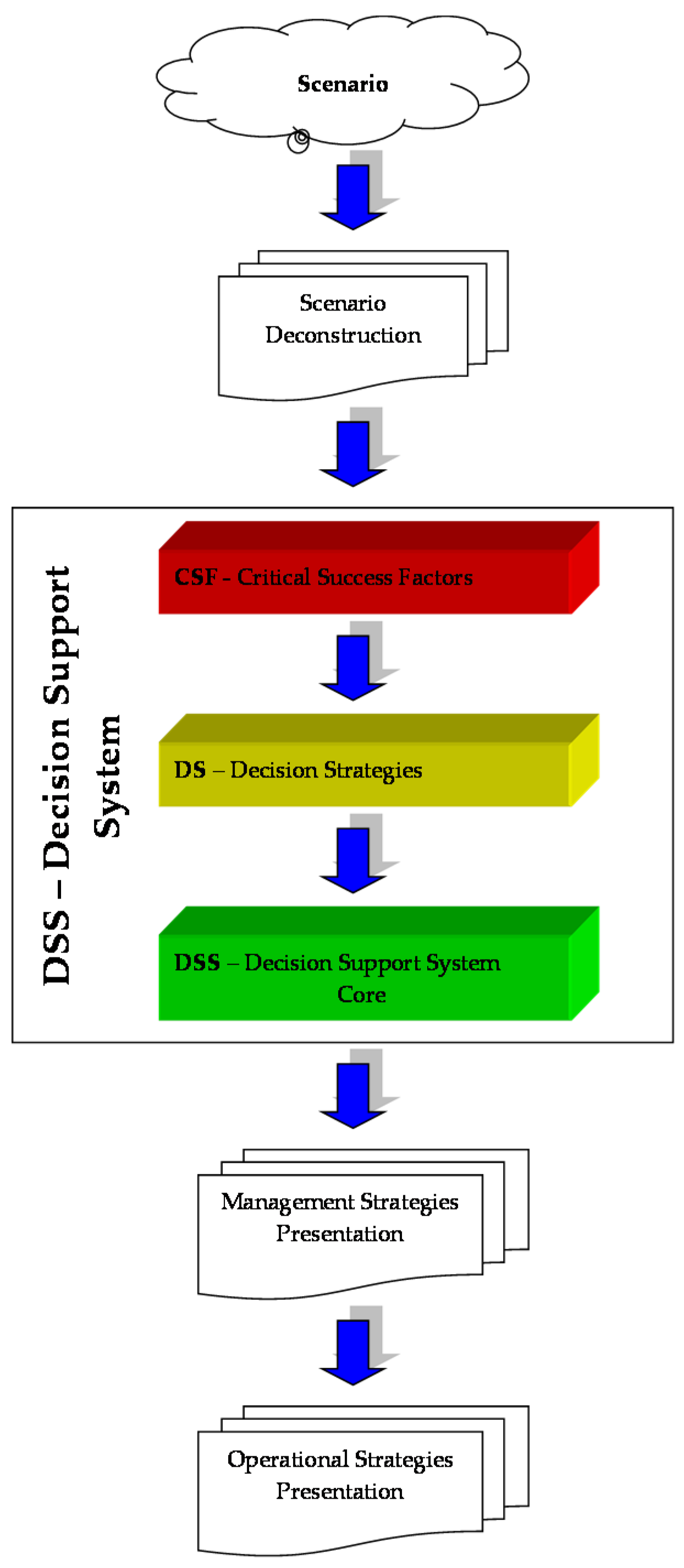
7. Decision Support System and Decisions Strategies

Thanks to the analysis described in the previous paragraphs, it is possible to associate each state, understood as a micro-state characterized by the seven CSFs, with a macro-state, i.e., a state characterized by the pair of state variables (S,E). With this completed, it is possible to either fix the variables of the physical hyper-dimension, i.e., latitude, longitude, and temporal location, or you can aggregate the data (the states) spatially, temporally, or spatio-temporally through the theory of moments with the creation of four indexes: (i) a position index (such as the arithmetic mean, the median or the mode); (ii) a dispersion index (such as the range of variation, the variance, the standard deviation); (iii) an asymmetry index; (iv) a kurtosis index. To better understand the usefulness of aggregation, think about having to make a decision which for a system does not concern a specific place corresponding to the latitude, longitude, and time coordinates, but which concerns the system in a complex system such as a neighborhood, city, work or social context, etc. We then understand the need for a greater level of synthesis. Once the macro-state, considered representative of the system, has been identified, immersed in the wider system in space and time, the purpose of the decision support system (DSS) will be to suggest a management strategy, i.e., an operational or governance strategy, which indicates how to manage the considered macro-state, i.e., the system state for a particular pair (S,E), to a more advantageous one. It should also be noted that transitions between micro-states within a macro-state are not the subject of this model. In fact, they would be equi-entropic and equi-energetic transformations, while the aim of the DSS is to suggest strategies that minimize (or reduce) entropy and maximize (or increase) internal energy.

The result is achieved through successive steps functional to the final aim. The final goal is the capture of the current state using one of the five fundamental attractors.

This aim can be achieved using different algorithms corresponding to different strategies. In other words, the system creates the following conceptual stack at three hierarchical levels:

• Identification of the seven CSFs (Critical Success Factor);
• Choice of decision strategy for the DSS;
• DSS computation.

Subsequently, the results of the DSS, i.e., those in a symbolic form (and in SE space), will be transformed via management strategies, i.e., codified in natural language accessible to all and simple to interpret, in order to implement the strategies of interest, i.e., in seven-dimensional original space (see Figure 8).

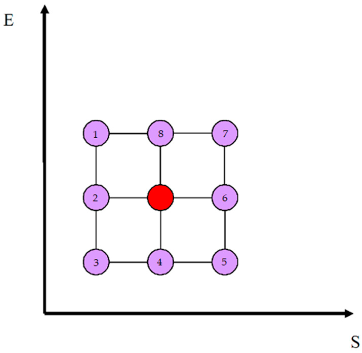
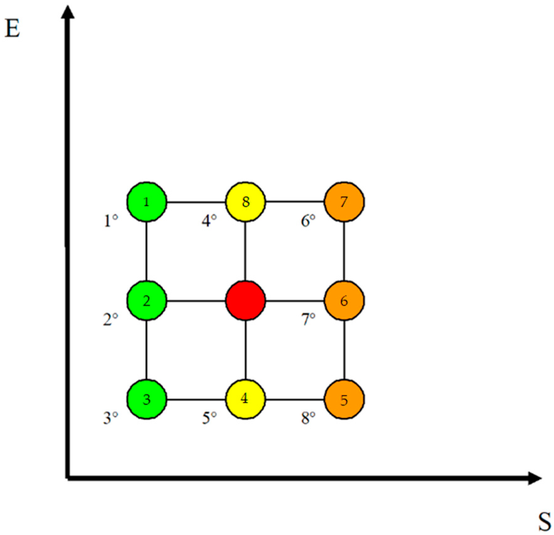
The strategy employed using the different algorithms has the objective of reaching one of the five attractors, i.e., minimizing entropy. This can be achieved through different decision-making strategies corresponding to different paths to follow in the SE plan. The objective is achieved by imposing the minimization of entropy until it is equal to zero. Since there are five fundamental attractors, there will be five privileged directions (global dominance). In fact, once points of coordinates (S,E) are fixed, we will have eight possible directions (local dominance) in relation to the three-by-three matrix centered on the state of interest and called an eight-connected (see Figure 9).

Let us consider a specific algorithm for minimizing the entropy. For each single step, this algorithm implements the following decision-making strategy through the hierarchization of priorities among the eight transformations (i.e., possible directions): 1, 2, 3, 8, 4, 7, 6, 5.

Therefore, the first priority is a transformation that leads to a state with lower entropy and greater energy (direction 1). If this is not possible because the state represented by the pair (S − 1, E + 1) is not permitted, the second priority is given using an isoenergetic transformation with entropy reduction (direction 2); the third priority is given to a transformation that reduces the entropy of the system by cooling it (direction 3). If none of the three previous transformations are allowed, it means that in the state the system is in, it cannot immediately transition into a state with lower entropy. Therefore, the global strategy attempts to break out of such a deadlock through an energy-increasing isentropic transformation (direction 8). If direction 8 is not possible either, the decision-making strategy tries again with an isentropic option, but this time with energy reduction and relative cooling of the system (direction 4). If it is not even possible to implement an isentropic transformation, it is essential to temporarily increase the entropy. In this case, the DSS tries to implement a strategy with energy increase first (direction 7); if this is not permitted, the decision system involves an isoenergetic transformation with an increase in entropy (direction 6); finally, if none of the previous transformations are permitted, the decision system ultimately implements the strategy corresponding to direction 5.

Overall, this decision-making strategy tends to minimize entropy by attempting to maximize energy. In any case, the dynamics are dominated by the minimization of entropy; in other words, the system always tries to reduce entropy first and chooses those with the highest energy among the possible meso-entropic transformations. From a formal point of view, there are three decision levels: (i) directions 1,2,3; (ii) directions 8,4; and (iii) directions 7, 6, 5. These directions ordered exactly in the indicated order create a global decision-making strategy in which the highest energy one is preferred among the meso-entropic transformations. For example, among 1, 2, and 3, 1 is preferred, then 2, and finally 3; between 8 and 4, 8 is preferred; and finally between 7, 6, and 5, on the first try 7 is preferred, which is the one with the highest energy of the three, and then the meso-energetic is preferred, that is, the 6, and finally the 5 is preferred, which corresponds to that with energy reduction.

Using traffic-light semantics, Figure 10 shows what has been described, where the first three choices are colored green, i.e., those corresponding to transformations with a reduction in entropy, isentropic transformations are colored yellow, while those with an increase in entropy are colored orange. The internal numbers of the state indicate the state itself, while the external numbers indicate their relative hierarchical ordering.

Figure 11 shows an example of the algorithm to minimize the entropy S and to increase the energy E. Figure 11 shows how the system, among billions of billions of possible paths (interconnections in red) in a clear regime of high complexity, is able to identify the decision-making path (white curve) that optimizes the state transitions in the entropy–energy plane.

A narrative approach provides an instantaneous representation of the system considered and under study. In order to make governance decisions, the decision support system presented must offer in sequence:

• A decision strategy (DS);
• A management strategy (MS);
• An operational strategy (OS).

Going into detail, the decisional strategy (DS) is a simulation of the system that allows us to move from a static to a dynamic vision. Thanks to it, in fact, the system, based on the choices of the decision-maker (for example the governance body), suggests a path for the SE (entropy–energy) plan to follow to achieve a specific objective, which in general is represented by a minimization of the entropy of the system and an optimization of the energy of the system itself based on the needs expressed. From a formal point of view, this is expressed with the trajectory of the SE plane. This trajectory is a broken curve whose ends of each segment provide information about the starting state (i.e., macro-state) of the system and the arrival state for each transition. Furthermore, the first initial state is the state of the system at the moment of the analysis, while the last is the objective state that is intended to be achieved through optimization. In order to build the decision-making strategy, the 78,125 micro-states in the SE plane are represented in terms of the 146 macro-states represented in Figure 12. Therefore each point representing a macro-state will be degenerated several times depending on the number of micro-states corresponding to it. Therefore, it is possible to construct a point intensity graph, like the one represented in Figure 13, so that each point is associated with a rectangle of a different color in relation to the density of micro-states corresponding to it.

Then, the management strategy (MS) suggests which actions to implement in terms of changes in energy and/or entropy. The last step provides the name of the attractor to be reached using the strategy, classified according to the following scheme in terms of entropy–energy pairs (S,E): (i) maximum attractor MA = (0.35), (ii) high attractor HA = (0.28), (iii) central attractor AC = (0.21), (iv) low attractor LA = (0.14), (v) minimal attractor mA = (0.7).

Finally, we will subsequently see the operational strategy (OS), which provides the actions to consider in terms of micro-states. In other words, once the different steps in the SE plan have been identified, i.e., the macro-states to be considered thanks to the DSs, with the MSs the management strategies are determined in terms of variations in S and E to be followed, with the OSs—based on the choices of the decision-maker and to the different OS that the system offers—the specific micro-states in which the system should transit are identified. Therefore, thanks to the Oss, it is possible to understand how to vary the system CSFs by acting directly on the seven different factors which are indicated (i.e., the DSS gives the results in terms of the CSFs of the micro-state in the initial seven-dimensional space). The decision-maker will, therefore, have operational support to govern the system using the mathematical modelling and operational strategies available, which are not only the result of experience but also of a careful analysis of the complexities to be managed.

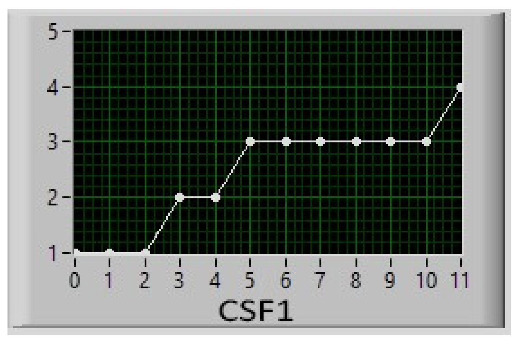
Figure 14 shows an example of CSF’s result, representing the dynamics in time (i.e., step by step). Consequently, we find the suggested behavior for each of the CSFs and, therefore, for the micro-states which is the variation towards reaching the final state. As mentioned in Section 2, in this example, the seven CFS are, respectively, a (1) demographic index, (2) environmental index, (3) economic index, (4) organizational index, (5) political index, (6) psychological index, (7) ethical index. For each CSF, the system indicates not only the final decision, i.e., the value in the range [1, 5] to be achieved, but also the decision-making trajectory, i.e., the changes in the value that each CSF must comply with in order to achieve the final decision/target.

8. Conclusions

In this study, a new methodology for analyzing information coming from any information source has been considered thanks to a DSS based on innovative methodology and seven dominant and independent CSFs—critical success factors. Starting from the space of possible scenarios, the system first clusters the information to obtain macro-analysis indexes capable of representing the system in terms of dynamism, i.e., energy, and organizational level, i.e., order and entropy. Thanks to this thermodynamic metaphor, it is possible to build deterministic models capable of building government logics which are not only the result of experience, but which are significantly supported by a system capable of suggesting decision-making strategies in relation to the identified priorities. Following this macro analysis, the model and the related system offer the user the possibility of identifying priorities in management terms; in this case, the information is dismantled again so as to be analyzed according to the specific needs of the user and offering management strategies. If this is still not sufficient, the computational model provides the possibility of requesting specific operational strategies which allow the definition of micro-states through which the system can pass without prejudice to the final target of reaching a given state of interest to which the system itself is to be led. The conceptual stack is as follows:

• Scenario modelling;
• Contextualization of the scenario in the spaces of all possible states;
• Identification of critical success factors;
• Definition/Identification of decision-making strategies;
• Definition/Identification of management strategies;
• Definition/identification of operational strategies.

This guarantees to the decision-maker the analytical ability to make the best choices, based on specific needs that arise from time to time.

For completeness of reasoning, it is useful to observe that if we jointly consider the 78,125 micro-states with their distribution, as shown in Figure 11, and the 6.665 × 10²⁴ trajectories produced using the unit of decision-making strategies, as shown in Figure 10, it can be deduced, after some calculation, that in the system in its entirety, suggesting the use of the optimal operational strategy with respect to the user’s requests, it processes a total number of cases (micro-trajectories) equal to 1.18 × 10³¹¹. To arrive at this number it is sufficient to appropriately multiply what is obtained in Figure 4 with what is reported in the table of the number of decision-making strategies, or trajectories between macro-states (see the following table from which the previous number is obtained by multiplying all the different factors together).

It is clear that when faced with such a number of possibilities (see

Table 10. Computational complexity of each moving step for reaching the target.

Transitions S → S − 1	Trajectories Between Microstates N.
12 → 11	3.7 × 1013
11 → 10	5.1 × 1021
10 → 9	8.1 × 1029
9 → 8	5.0 × 1037
8 → 7	2.5 × 1044
7 → 6	1.8 × 1049
6 → 5	5.6 × 1050
5 → 4	2.4 × 1021
4 → 3	2.6 × 1019
3 → 2	5.4 × 107
2 → 1	3.2 × 103
1 → 0	5.6 × 10

), one either relies on common sense by choosing according to experience or one must rely on an advanced decision support system such as the one proposed, based on the complexity theory. The first approach is obligatory if one does not have a model and a system like the one proposed, which has the advantage of transforming into a deterministic/rational decision that could otherwise be subjective in a context that could apparently appear chaotic, but which is instead only extremely complex. A system like the one proposed is a very powerful analysis tool and an effective and efficient tool as well as flexible, with multi-resolution, and being adaptable to specific needs for decision support.

A support expresses itself in decision-making, management, and operational support in relation to the needs expressed, the choices made, and the objectives that are intended to be achieved.

The solution proposed in this article is one that is capable of handling such high levels of complexity. The most important intuition was probably to create a specific algorithm to move from a seven-dimensional space to a two-dimensional one, where computational complexity is reduced. At this point, a second algorithm allows us to return to the initial seven-dimensional space, solving the problem of degeneration due to the transition from two to seven dimensions. In this way, the system is able to provide a decision-making path in seven dimensions, with a very low computational cost, showing a viable path to problems that were previously computationally intractable with current technologies and that probably only quantum computing could have addressed.

Although the proposed solution can find application in the most varied contexts, typical application examples could be used for territorial control; for the analysis of criminal phenomena and security; for the optimization of trajectories for logistics and transport companies; for the psychological profiling of customers; for the psychological profiling of employees of a large company; for the monitoring of threats to an information system; and for artificial intelligence systems which intend to consider not only the structural components (neural networks), but also neuronal conditioning with inhibitory or excitatory effects, etc.