Triple Time Interval Hybridization Strategy for Rapidly Calculating Regional Target–Visible Time Window of Earth Observation Payloads on Space Station

Abstract

Earth observation payloads deployed outside the space station play a pivotal role in remote sensing and atmospheric monitoring. Calculating the visible time window (VTW) for regional targets is a fundamental aspect of payload observation and operational mission planning. Aiming to address the challenge of rapidly calculating the VTW for regional targets, this paper introduces the Triple Time Interval Hybridization Strategy (TTIHS). By integrating orbit filtering, large-step angle calculation, and a short interval binary search, the TTIHS adapts different strategies within global, coarse search, and precise search time intervals, effectively reducing computational workload and improving speed. Simultaneously, optimization analysis is conducted on the time step in the coarse search, achieving a balance between computation speed and accuracy. Simulation results, based on real data from the China Space Station, highlight a significant improvement in computational speed while ensuring accuracy. Specifically, the proposed rapid algorithm exhibits a 2.73-fold enhancement in speed compared to the existing rapid algorithm.

1. Introduction

External payload platforms outside the space station support multidisciplinary space science research, encompassing Earth observation, space astronomy, radiation biology, material exposure, and new technology tests [1]. Earth observation from the space station, characterized by low orbital altitude, multiple time windows, high spatial resolution, and varying lighting conditions, serves various purposes such as remote sensing, resource surveying, disaster assessment, weather forecasting, and climate change monitoring [2]. Constrained by the orbital altitude, payload field of view, and target imaging conditions, the continuous observation of targets is limited, achievable only when the field of view intersects with targets, known as the visible time window (VTW) [3]. For large-scale space science payloads, it is imperative to calculate their VTW to determine operational modes. Therefore, VTW calculation is crucial for payload mission planning, setting the foundation for mission activities [4,5]. Research on VTW calculation is significant for rapid determination, particularly for emergency and real-time planning, and accurate VTWs enhance planning efficiency by reducing planning margins [6,7].

The crux of the VTW calculation problem is determining the relationships among spatial points, lines, and areas. Research has progressed from the tracking and propagation (TP) method to more rapid algorithms. TP, a classical approach, involves continuously tracking a trajectory at fixed time intervals [8]. This involves computing the orbit positions and determination of the payload’s visibility to the target at each sampled moment, yielding the VTW. While TP provides accurate results, its time-consuming nature poses challenges, especially for time-constrained planning tasks. Nonetheless, it remains a benchmark for its accuracy.

To expedite computations and address various targets, rapid algorithms are proposed, mainly including numerical and geometric methods. The former focuses on solving the intersection information as a function of time, while the latter calculates the geometric relationship between the projection and the targets. Numerical methods derive analytical formulas for VTWs from spacecraft–target relationships, solving transcendental equations based on Kepler’s theory. These methods employ approximation techniques like Newton’s method to reduce computation time and avoid multiple solutions to Kepler’s equation. Key methods include the eccentricity function method, visibility function method, sub-point trajectory method, and Poincaré mapping method. Escobal [9] introduced a transcendental equation using the eccentricity function, obtaining a closed solution for two-body motion through interpolation. Lawton [8] proposed a visibility function method based on the Fourier series, further improved by Alfano et al. [10] using parabolic hybrid technology. Nugnes [11] proposed a visibility function transcendental equation for satellite coverage, and Katona [12] defined a general expression of the function for a single satellite concerning ground position. Ali et al. [13] proposed the sub-point trajectory method, approximating it within the orbit period using the same orbit great circle. Sengupta et al. [14] proposed an analytical form based on the Poincaré mapping method, while Sun et al. [15] enhanced it with adaptive interpolation technology. Han et al. [16] proposed a rigorously adaptive Hermite interpolation method for function curve fitting, and Wang et al. [17] transformed the problem into a multi-peak function root-finding problem, approximating the visibility function based on various modeling techniques. Geometric methods employ orbit ergodic search to determine the geometric relationship between the field of view and targets to obtain the VTW, with a simple model and low complexity. Plamer et al. [18,19] proposed a coarse and precise search method, using a two-body and complex models to obtain an approximate and precise time, respectively. Feuerstein [20] adopted orbit filtering to exclude cycles without VTWs. Ulybyshev [21] proposed a geometric method based on 2D maps. Coarse and precise search concepts enhance speed and offer insights for further research.

Previous research mainly addressed point targets, while computing for regional targets poses challenges due to irregular polygons. Various methods have emerged for regional targets like boundary intersection, boundary discretization, and grid matching. E et al. [22] used boundary intersection and coarse/precise search, while Han [23] and Bai [24] solved the intersection problem using geometric methods. E et al. [25] suggested a method combining coarse calculation with a precise binary search based on boundary discretization. Song et al. [26] proposed a grid method, discretizing regional targets into a grid and traversing to identify covered grid moments. Wang et al. [27] introduced a method based on map segmentation, traversing sub-points within a specific range by segmenting maps and trajectories. However, for large-scale payload systems in mission planning, the VTW is repeatedly invoked, and the emergence of regional targets also poses a challenge. Therefore, there is a need to enhance the speed and accuracy of existing methods.

Efficient VTW calculation with minimal computational consumption and high accuracy is crucial. This paper introduces the Triple Time Interval Hybridization Strategy (TTIHS) for rapid VTW calculation of regional targets. The TTIHS integrates orbit filtering, large-step angle calculation, and short interval binary search strategies, employing different strategies in various intervals to enhance computational speed. In addition to the coarse and precise search phases in previous algorithms [25], the TTIHS introduces an orbit filtering phase before the coarse search, mitigating the time-consuming iteration of calculating visibility for each position in global time, a drawback of previous algorithms. After filtering, a large-step angle calculation strategy is employed within the filtered interval and a short interval binary strategy rapidly calculates the start-end times of the VTW. The challenges in developing this algorithm are twofold. One is determining the time range for the orbit filtering, which is addressed by introducing the concept of an extended rectangle based on the four-boundary range. The other is parameter selection, where an optimized analysis of the time step is conducted to establish the relationship between computational accuracy and the step. The paper makes three key contributions: proposing the TTIHS framework, introducing an orbital filtering method using extended rectangles, and conducting a comparative analysis of algorithm performance with parameter optimization for the time step. Its structure consists of a first part introducing the study’s significance and research status, a second part presenting the preliminary work, a third part detailing exposition of the TTIHS model, a fourth part discussing the outcomes and results analysis, and a fifth part providing conclusions and potential avenues for future research.

2. Preliminary Work

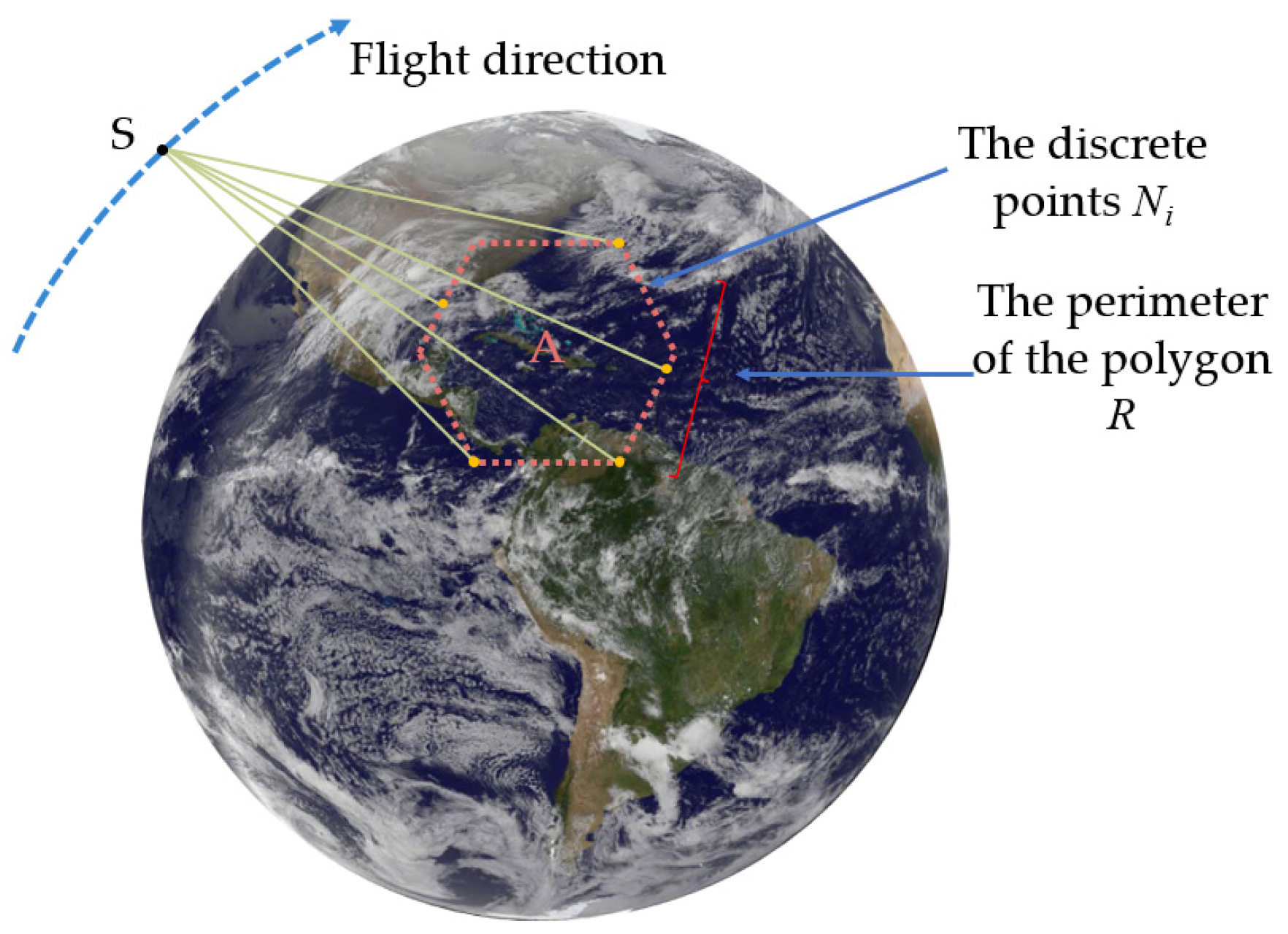
2.1. Theoretical Foundation

The theoretical foundations for VTW calculation for Earth observation payloads involve spacecraft orbital dynamics, space geometry, and related principles. The calculation process entails inputting data such as space station orbital information, payload parameters, and observation target details to output the VTW [28]. Orbital data describe the spatial position of space station over a period, typically obtained by providing Two-Line Element (TLE) data as initial parameters and utilizing precise orbit propagation models such as SGP4 and SDP [29]. This yields accurate Earth-centered inertial coordinates (x, y, z) and velocities (v_x, v_y, v_z) at a given time. The SGP4 model is commonly used for near-Earth orbits due to its high predictive accuracy [30]. The visibility range of the payload is influenced by the payload’s field of view type, commonly characterized by conical or rectangular fields of view [31]. The observation target region is generally represented as a closed polygon with a broad coordinate span that cannot be covered by a single instantaneous field of view or scanning strip of the payload. A schematic diagram of a VTW is shown in Figure 1, where the circular region M represents the circular field of view projection of the payload, the blue rectangle N represents the ground regional target, and the dashed line represents the sub-point track. Based on the given information, the geometric relationship between the current moment’s projection region M and the regional target N is determined. Starting from the initial time, it is assumed that the regions M and N are disjointed. When at time a, they intersect, marking the start of timing, and this continues until time b when they separate, marking the end of timing. The duration between these two critical times a and b represents the VTW of the payload for target N [32].

The specific approach for calculating the VTW involves using the payload’s orbital position information and the latitude and longitude information of the ground region. It calculates the angle (referred to as β in Figure 2) between the line connecting the sub-point and the payload and the line connecting the target and the payload, along with the payload’s half field of view angle (referred to as α in Figure 2). This is illustrated in Figure 2, adopting the spherical Earth model with O as the Earth’s center, S as the space station platform (payload), L as the target position, and T as the intersection point between the payload-to-Earth’s-center line and the ground. The three orange lines, LO, SO, and SL, form a triangle. Here, ST represents the height of the space station orbit h, TO represents the radius of the Earth r, and LO represents the distance from the ground target to the Earth’s center. Q is the intersection point between the payload’s field of view and the ground. Assuming the accuracy of the space station’s orbital position obtained based on the TLE and SGP4 models, firstly, based on the space station’s position, the position of the sub-point T is calculated. The central angle ε between point T and the ground point L (lon_L, lat_L) is then determined. Subsequently, using this angle and the lengths of the two sides, the length of side SL b is calculated using the law of cosines. Finally, the angle β between sides SO and SL is determined using the law of arcsines. By comparing this angle β with the payload’s half field of view angle α, if β is less than or equal to α, then the target is within the visible range. The position of point T is recorded at this moment. The corresponding time is calculated as the start time of the VTW, denoted as ‘T_a’, and it continues until β starts to exceed α. Similarly, the position of point T is recorded at this moment and denoted as ‘T_b’. Therefore, the VTW of the payload to point L is [T_a, T_b] [33].

The specific calculation steps can be divided into three parts: the coordinate transformation, calculation of angle β, and determination of the critical angle β₀ and corresponding time T_i. Firstly, to maintain consistency in the coordinate systems and facilitate the calculation of the angle ε and β, the latitude and longitude of the ground points need to be converted into three-dimensional coordinates in the Earth-centered inertial coordinate system, according to the conversion formula shown in Formula (1) [34].

$$\begin{array}{c}{x}_L=r\cos (la{t}_L)\cos (lo{n}_L)\\ y_L=r\cos (la{t}_L)\sin (lo{n}_L)\\ z_L=r\sin (la{t}_L)\end{array}$$

(1)

where r represents the radius of the Earth, and lat_L and lon_L, respectively, denote the latitude and longitude of the ground point L. Based on the unified coordinates of the two points, the angle ε and β can be calculated using Formula (2).

$$\begin{array}{c}\epsilon =\arccos (\frac{\mathit{u}\cdot \mathit{v}}{‖\mathit{u}‖\cdot ‖\mathit{v}‖})\\ b^2={(h+r)}^2+r^2-2\cdot (h+r)\cdot r\cdot \cos (\epsilon )\\ \beta =\arcsin (\frac{r}{b}\cdot \sin (\epsilon ))\end{array}$$

(2)

Here, u = (x_T, y_T, z_T) denotes the geocentric coordinates of the sub-point, v = (x_L, y_L, z_L) represents the geocentric coordinates of the ground point, “·” denotes the dot product operation, and ‖·‖ represents the magnitude of the vectors. h and r, respectively, stand for the orbit altitude and the radius of the Earth. Based on this, critical angle determination is performed. Starting from the initial moment, the angle β is computed continuously at each moment, recording the time when each orbit’s β_Ti = α, as shown in Formula (3). The T_i moments are merged, and the earliest and latest T_i are selected to obtain the VTW [T_is, T_ie] for each orbit regarding region N.

$$\begin{array}{c}{\beta }_{Ti}=\alpha \\ VT{W}_n=[T_{is},T_{ie}]\end{array}$$

(3)

By employing the previously described angle and orbit calculations, the VTW of the payload for the target can be computed, utilizing the input target position and spacecraft orbit information. The subsequent models are all constructed on the foundation of this theoretical calculation.

2.2. Mathematical Analysis

The general approach for calculating the VTW for regional targets involves discretizing the region into several points, computing the VTW for each discrete point at each time step, and then merging these to obtain the VTW for the global regional target. The combined coarse and precise search method is currently a widely used rapid algorithm [25,35], which involves traversing each time step first with a large step angle calculation and then using a binary precise search to improve computational speed. However, further analysis reveals optimization potential in this method. As illustrated in Figure 3, the dashed lines represent the sub-point track, red star represent ground regions, black rectangular frames represent rectangular regions covering ground regions, and solid lines inside the rectangles represent valid sub-point tracks. When traversing the global time interval with large steps, angle calculations for each discrete point at every time step are required, involving nested traversal and a high number of computations. If this step can be shortened to a smaller time interval, as in the rectangle, reducing the nested traversal to only that interval, it will significantly reduce the number of computations. This involves first calculating the sub-point position using the orbital model, then conducting coarse search nested traversal within a smaller interval, and finally performing the binary search. In the following analysis, this approach is referred to as the “new approach”, while the coarse and precise search is termed the “original approach”. The computational complexity analysis of both approaches will be discussed below.

According to the big O notation for calculating time complexity analysis [36], the computational complexities of the original approach and the new approach are denoted as T_o(n) and T_x(n), respectively, with the computation formulas as shown in Formula (4).

$$\begin{array}{c}{T}_o(n)=\max (O(n_a\cdot m),O(\log n_c))\\ T_x(n)=\max (O(n_a),O(n_b\cdot m),O(\log n_c))\end{array}$$

(4)

In the former formula, O(n_a·m) represents the computational complexity of the coarse search phase in the original approach, where n_a denotes the number of sampling traversals within the global interval, m represents the number of discrete points in the polygon, and O(log n_c) indicates the complexity of the precise search phase within a short time interval, where n_c represents the number of binary searches within the short interval. In the latter formula, O(n_a) denotes the complexity of the traversing and computing positions within the calculation interval in the new approach, while O(n_b·m) represents the complexity of the coarse search phase, where n_b denotes the number of traversals within the smaller interval. The complexity of the binary search phase remains the same as before. From the above analysis, it can be inferred that the nested traversal is the part with the higher complexity. In comparison to the original approach, n_b is significantly less than n_a, indicating that the coarse search phase in the new approach involves fewer nested traversals and a significant reduction in computation, thereby improving computational speed. The algorithm proposed in this paper is thus based on this mathematical and theoretical foundation, achieving an increase in computational speed by reducing the number of computations.

3. Method

3.1. Basic Idea

The geometric principle underlying the VTW involves determining whether the projection region intersects with or separates from the target. Since the VTW is only a small portion of the global calculation interval, it is evident from the process that boundary discretization and angle calculation are also required during the separation times. However, the angle calculation during the separation phase can be considered as unnecessary computation. This part of the computation would increase the amount of computation time. Assuming the accuracy of the orbit propagation model, if it is possible to predict the time of the separation and intersection based on the orbit position information, excluding ineffective time, then boundary discretization, angle calculation, and calculations are necessary only within the vicinity of the window. This approach ensures an improvement in computational speed while maintaining calculation accuracy. Therefore, this paper proposes an orbit filtering method based on an extended region, as illustrated in Figure 4. In the figure, the orange circular part D represents the payload’s field of view projection, S is the sub-point, and m is the radius of the projection. The irregular blue region is the ground target region A, the rectangular line region B is obtained by expanding A based on the four extreme points range, and the rectangular dark blue region C is obtained by expanding region B with the radius m of the field of view projection D. Thus, it is necessary to determine only the relationship between the sub-point S and region D, transforming the positional relationship judgment between the regions into a judgment between a point and a region. In Figure 4a–c, regions C and D are shown in different scenarios as follows:

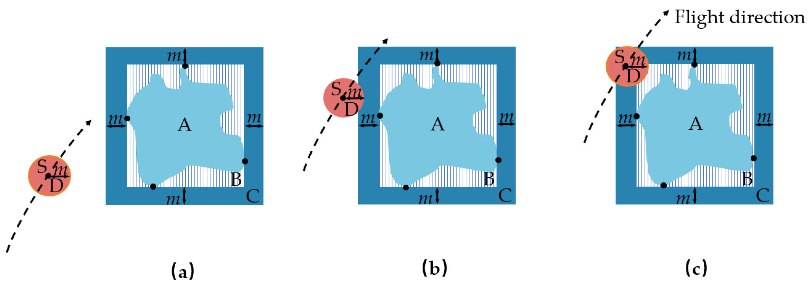
(1)

In case (a), regions C and D are separate, with region C not containing point S;

(2)

In case (b), regions C and D intersect, with region C not containing point S;

(3)

In case (c), regions C and D intersect, with region C containing point S.

In situations (a) and (b), regions D and A are not intersecting, while only in situation (c) is there a possibility of intersection between region D and A. Therefore, this approach can effectively exclude cases where there is no intersection, specifically by determining the positional relationship between the sub-point S and the expanded region C.

Building upon the extended region, the paper introduces the TTIHS. As depicted in Figure 5, gray represents the time intervals, golden arrows indicate the interval lengths, red, blue, and green, respectively, represent the orbit filtering, large-step angle calculation, and small-interval binary search strategies adopted in the global time interval Δt₁, the coarse calculation time interval Δt₂, and the precise calculation time interval Δt₃. The time intervals form a pyramid structure from bottom to top, indicating the gradual shortening of the calculation time intervals. The first step involves employing the concept of an expanded rectangle within the global time interval [t_1s, t_1e] (Δt₁) to implement an orbit filtering strategy. Utilizing the longitude and latitude of rectangle C and the orbit model, the times where point S is not within rectangle C are excluded. This phase requires only the calculation of the orbit position, effectively eliminating a large range of non-visible time intervals to reduce computation. This results in the coarse calculation time interval [t_2s, t_2e] (Δt₂). Within Δt₂, a large-step angle calculation strategy is employed, calculating the angle relationship between the sub-points and boundary discretization points. This yields a precise calculation time interval [t_3s, t_3e] (Δt₃). Finally, based on a short interval binary search strategy, the start -end times of the VTW are quickly calculated, thus obtaining the complete VTW.

The specific calculation process of the algorithm is illustrated in Figure 6, where the same three colors of red, blue, and green represent three different calculation strategies, as shown in Figure 5. Initially, orbit segmentation is carried out based on the input information. In this phase, region expansion is performed. Subsequently, position calculation is conducted to determine whether the sub-point has reached the boundary of the expanded region. The corresponding circle and start-end times are recorded. In the coarse calculation phase, the regional boundary is uniformly discretized to realize the angle calculation of the payload’s view field and the point. A large-step angle calculation is employed to roughly calculate whether the angle within the time interval is equal, and intervals that meet the requirements are recorded. In the precise calculation phase, only a certain precision is used for the binary calculation. The precision is checked to determine whether it meets the requirements, and intervals that meet the requirements are recorded as the VTW for the global mission interval. The pseudo code for the algorithm is shown in Algorithm 1.

Algorithm 1: Compute Visible Time Window
	Input: TLE, the orbit data. α, the payload parameters.                (Loni, Lati), the observation target information.
	Output: VTW, the visible time window.
1	Initialize control parameters and data structures.
2	Perform time and orbit segmentation.
3	Expand the boundaries based on the orbit information.
4	Orbit Position Calculation:
5	while The circleall have not been all traversed do
6	if the satellite position reaches the boundary region then
7	Record the corresponding orbit circle-filtered and
	start/end time Δt2.
8	else
9	continue to the next time.
10	end
11	end
12	Discretize the boundary region
13	Angle Calculation:
14	while The circle-filtered have not been all traversed do
15	if the angle satisfies the requirements then
16	Record the corresponding orbit circle-coarse and
	start/end time Δt3.
17	else
18	continue to the next time.
19	end
20	end
21	Binary Calculation:
22	while The circle-coarse have not been all traversed do
23	if The precision criteria are met then
24	Record the final time.
25	else
26	repeat the binary search.
27	end
28	end

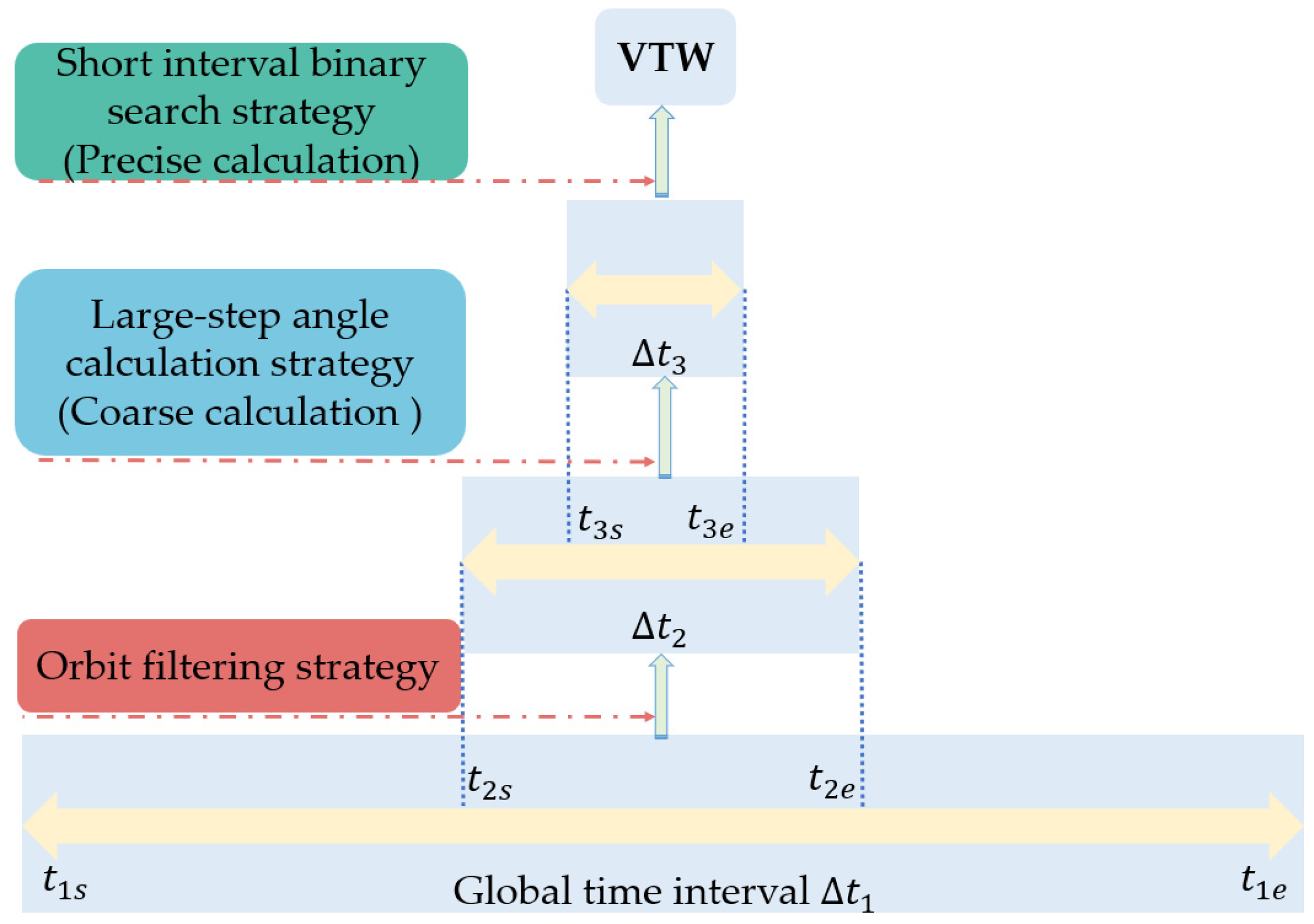
3.2. Algorithm Steps

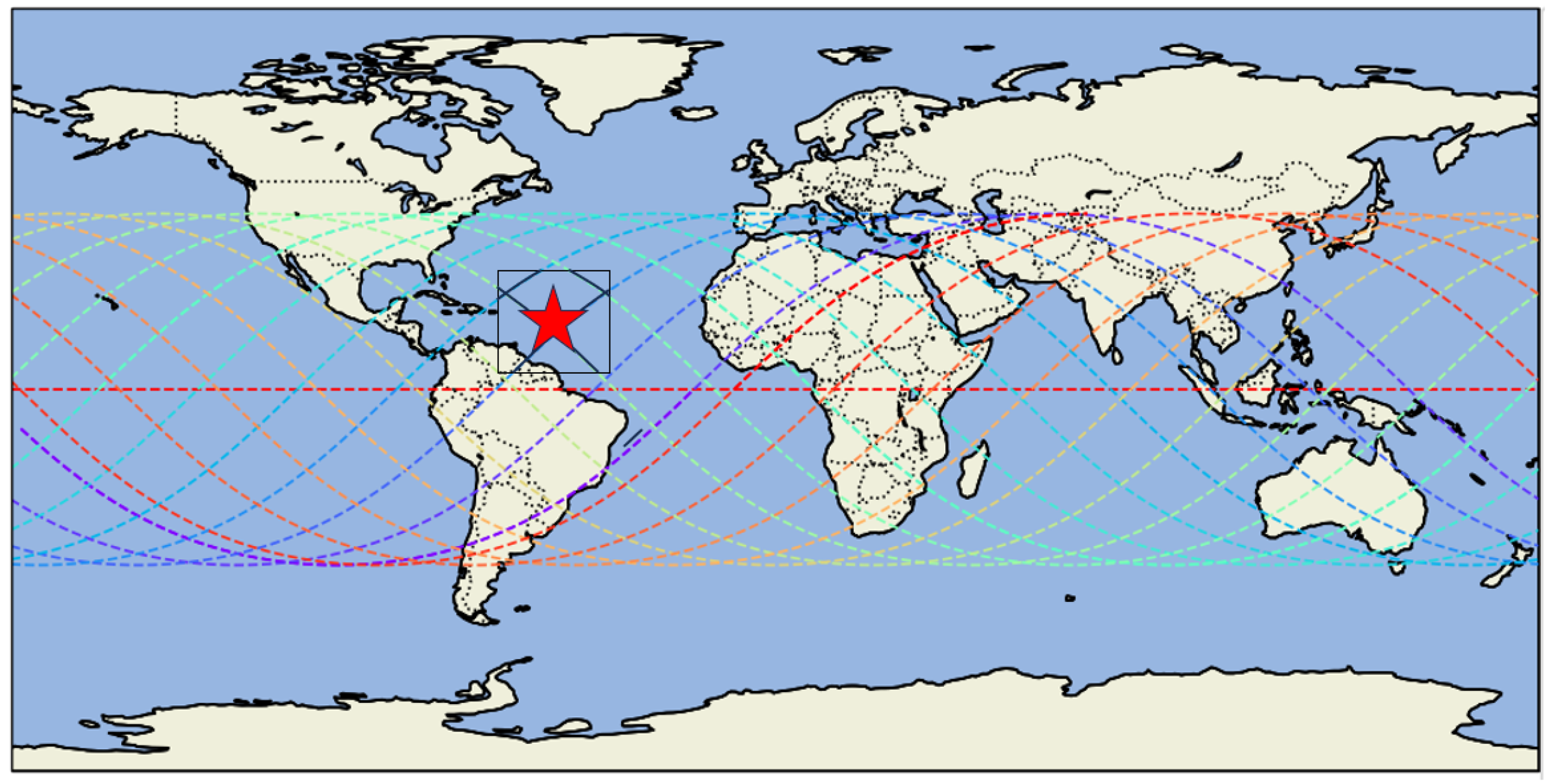
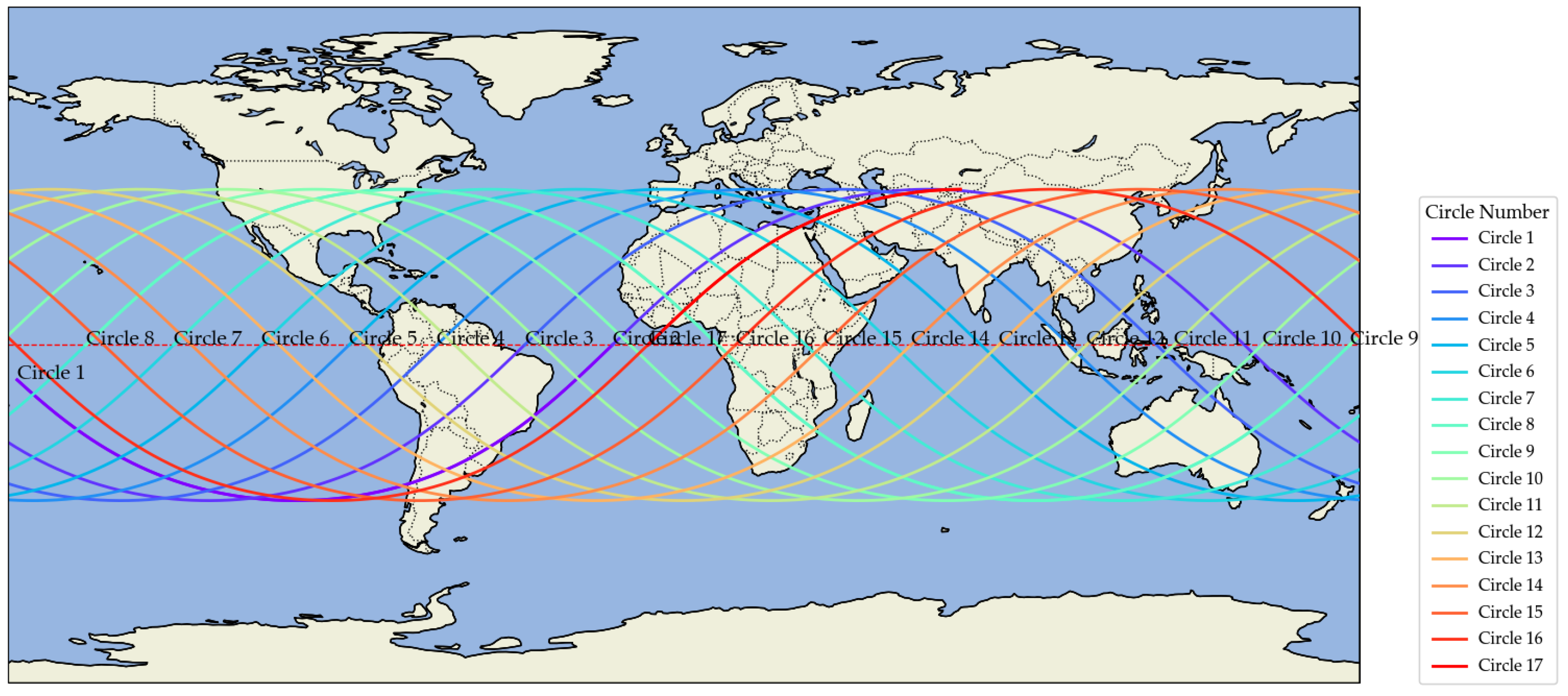
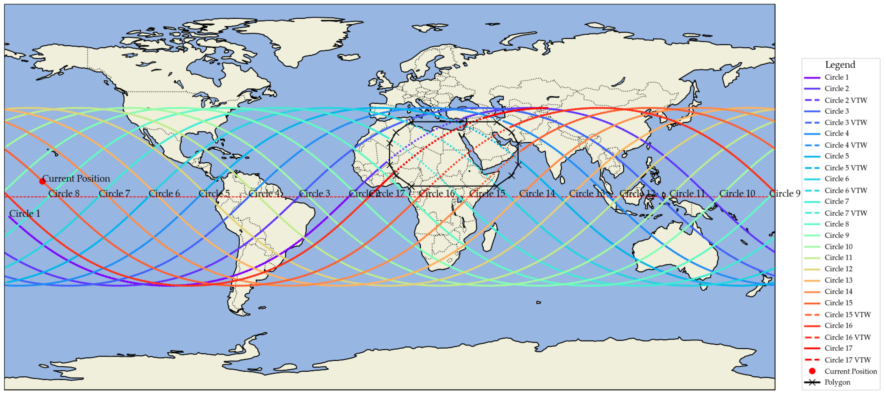
3.2.1. Orbit Filtering

This section mainly involves orbit segmentation, region expansion, and calculation of the intersection time interval between the expanded rectangle and the sub-point, to achieve orbit filtering and exclusion of large-scale invalid times, and to obtain the approximate time interval of the VTW. The main steps include orbit segmentation, region expansion, and position calculation.

Step 1: Orbit Segmentation. First, the orbits within the global time interval Δt₁ are segmented into circles. The circles are numbered based on two consecutive passes of the sub-point over the equator, and they are sequentially ordered by time. As shown in Figure 7, Circle 1 starts from the beginning of the interval (t_1s) until the sub-point passes the equator for the first time, indicated in blue. Circle 17 extends from the last time the sub-point passes the equator to the end of the interval (t_1e), indicated in red. The intermediate circles are defined by consecutive two passes of the sub-point over the equator [t_si, t_ei], and different circles are marked with different colors [25].

Step 2: Region Expansion. Based on the location information of the ground target and the orbit calculation model, the four limit points of the target are obtained, i.e., V(lon_v, lat_v), W(lon_w, lat_w), Y(lon_y, lat_y), and U(lon_u, lat_u). Next, the four latitude and longitude values are determined, and a rectangular region C is expanded, as shown in Figure 8. The coordinates of its four vertices are E(lon₁, lat₁), F(lon₂, lat₁), G(lon₂, lat₂), and H(lon₁, lat₁). The coordinate calculation formula is given by Formula (5).

$$\begin{array}{c}lo{n}_1=lo{n}_u-\epsilon \\ lo{n}_2=lo{n}_w+\epsilon \\ la{t}_1=la{t}_v-\epsilon \\ la{t}_2=la{t}_y+\epsilon \end{array}$$

(5)

Step 3: Position Calculation. The relationship between the sub-point S (lon_s, lat_s) and the expanded rectangle C is determined. This involves iterating through the longitude and latitude of the sub-point at each time step to check if they fall within the coordinate range of the extended region. For instance, if the longitude lon_s1 of the sub-point S₁ is within [lon₁, lon₂], but its latitude lat_s1 is not within [lat₁, lat₂], then it is not inside the extended region. Conversely, for point S₂, if its longitude lon_s2 is within [lon₁, lon₂] and latitude lat_s2 is within [lat₁, lat₂], then it is inside the extended region. Formula (6) represents the position judgment formula [37]. By iterating through each time step, a collection of sub-points located within the extended region can be obtained, and their corresponding time intervals are recorded to derive the Δt₂ during which they are inside. This process effectively eliminates sub-points outside the extended region range, thereby achieving the orbit filtering process.

$$\begin{array}{c}lo{n}_1\le lo{n}_s\le lo{n}_2\\ la{t}_1\le la{t}_s\le la{t}_2\end{array}$$

(6)

Through the above two steps, it is possible to filter out the large time interval when the two regions are separated, reducing the global computation time Δt₁ to a relatively small interval Δt₂.

3.2.2. Coarse Calculation

This section mainly involves boundary discretization and calculating the angle relationship between the sub-points and discrete points on the boundary within the vicinity of the VTW. The goal is to determine the start-end times of the VTW. The main steps include boundary discretization and angle calculation.

Step 4: Boundary Discretization. As shown in Figure 9, the regional target A is discretized into red equidistant points N_i [25]. The approach involves obtaining the length R of the polygon based on the latitude and longitude of the polygon vertices. The distance between each discrete point is then determined as R/N_i, and the latitude and longitude of each discrete point are calculated accordingly through linear interpolation [38]. The angle β_i between the payload and each discrete point is computed, and the minimum angle β_min among the discrete points is selected as the angle β_t between the payload and the polygon region at the current time. The formula for calculating the length of the polygon R is given by Formula (7), where r is the radius of the Earth and (lon_Li, lat_Li) represents the coordinates of each vertex of the polygon.

$$R={\displaystyle \sum _{i=1}^{n-1}r\cdot \arccos (\sin (la{t}_{Li})\cdot \sin (la{t}_{Li+1})+\cos (la{t}_{Li})\cdot \cos (la{t}_{Li+1})\cdot \cos (lo{n}_{Li+1}-lo{n}_{Li}))}$$

(7)

Step 5: Angle Calculation. Within the time interval Δt₂, a large-step t_d is used to traverse and calculate the relationship between the angle β_t and the half-field angle α. If the angle β_t changes from greater than to less than α, it is considered the starting point T_3s of the VTW. Subsequently, if there is a process of transitioning from being less than to greater than and then back to being less than α, and if β_t changes from less than to greater than α, it is considered the endpoint T_3e of the VTW. This process determines the interval Δt₃.

3.2.3. Precise Calculation

This section mainly builds upon the coarse calculation of the start-end times of the VTW using the binary search method to precisely determine the start-end times. This means that given the existence of start-end times within the t_d interval, this section precisely determines those moments.

Step 6: Binary Calculation. This section computes only the angle relationship within the start time interval [T_3s, T_3s + td] and the end time interval [T_3e, T_3e + td] of Δt₃, using α as a reference and employing a certain precision λ for the binary search. Taking the start time as an example, within the VTW start time interval [T_3s, T_3s + td], if the angle β_t at (T_3s − T_3e)/2 exceeds α, indicating the payload is still not visible to the target, (T_3s − T_3e)/2 is set to T_3s for further computation; conversely, if β_t at (T_3s − T_3e)/2 is less than α, (T_3s − T_3e)/2 is set to T_3e for further computation until the precision λ requirement is met. This moment is then considered the start time of the VTW. Similarly, the end time can be obtained, thus deriving the entire precise VTW. The calculation formula is as shown in Formula (8), where β((T_3s − T_3e)/2) represents the β value at (T_3s − T_3e)/2 time [39].

$$\left\{\begin{array}{cc}(T_{3s}-T_{3e})/2=T_{3s},& if\beta ((T_{3s}-T_{3e})/2)>\alpha \\ (T_{3s}-T_{3e})/2=T_{3e},& if\beta ((T_{3s}-T_{3e})/2)<\alpha \end{array}\right.$$

(8)

4. Results and Discussion

4.1. Evaluation of the Algorithm Performance

This paper utilizes the calculation results obtained through the TP method as a baseline and compares them with both the TP method itself and existing rapid algorithm, specifically focusing on the coarse search and binary search phases [25]. Simulations were conducted to validate the accuracy and superiority of the TTIHS algorithm. The China Space Station (CSS) was chosen as a case study, featuring an external payload platform that supports multiple Earth observation payloads. A randomly chosen twelve-sided polygon served as the ground polygon region, and the experimental parameter settings are detailed in

Table 1. The experimental parameter settings.

Category	Parameter
Payload	CSS Earth observation payload
TLE [40]	48274U 21035A 23357.28655182 .00041146 00000 + 0 42316-3 0 9997
	48274 41.4711 83.9203 0005576 41.6976 318.4288 15.64081887151409
Simulation time	23 December 2023 00:00:00–23 December 2023 24:00:00 (UTC)
Time step	ta = 1 s, tb = 90 s, td = 90 s
Half field of view angle	30°
Region coordinates	(5° N, 10° E), (5° N, 50° E), (10° N, 57° E), (15° N, 60°E), (25° N, 60° E), (30° N, 57° E), (35° N, 50° E), (35° N, 10° E), (30° N, 3° E), (25° N, 0° E), (15° N, 0° E), (10° N, 3° E)

. The simulation period extended from 00:00 to 24:00 (UTC) on 23 December 2023. The orbit model applied was the SGP4 model, and the Earth observation payload’s field of view type was conical with a half angle of 30°. To ensure fairness in the computations, all three algorithms were implemented under identical hardware and software environments. Details of the simulation environment setup are provided in

Table 2. Simulation environment setup.

Category	Information
Hardware environment	Intel (R) Core (TM) i3-10110U CPU @ 2.10 GHz Processor, 8 GB RAM, 223 GB storage
Operating system	Windows 11, X64-based PC
Software environment	PyCharm2023.2.5 (Community Edition), Python 3.10, PyEphem

. The calculation time step for the TP algorithm was denoted as t_a and set to 1 s, while for the existing rapid algorithm, it was denoted as t_b with the coarse search phase set to 90 s and the binary search precision set to 0.0005. The TTIHS algorithm’s calculation time step was denoted as t_d, with the coarse search phase also set to 90 s and the binary search precision set to 0.0005.

Figure 10 illustrates a schematic diagram of the simulated VTW, with different circles represented by distinct colors. The VTWs for the regional target are denoted by dashed lines, while the invisible intervals are indicated by solid lines. The red dot symbolizes the current position of the space station platform, and the black dashed line represents the ground polygonal region. The figure reveals a total of 17 circles within one day of simulated time. Among them, only Circles 2, 3, 4, 5, 6, 7, 15, 16, and 17 exhibit a VTW. A significant portion of the time lacks a VTW, underscoring the importance of the orbit filtering and coarse search in this method.

Table 3. Comparison table of computational time for different algorithms.

Algorithm	Computational Time/s	Computational Time Ratio t%
TP algorithm T0	31.728	100%
Existing algorithm T1	0.317	0.999%
TTIHS algorithm T2	0.116	0.365%

provides details of the simulation computation times for the three algorithms, while

Table 4. VTW information.

	TP Algorithm		TTIHS Algorithm
Identification Number	StartEnd Times	Duration/s	Start–End Times	Duration/s
1 (Circle 2)	00:48:29–00:58:54	00:10:25	00:48:29–00:58:54	00:10:25
2 (Circle 3)	02:29:21–02:30:35	00:01:14	02:29:20–02:30:34	00:01:14
3 (Circle 4)	04:14:46–04:15:56	00:01:10	04:14:46–04:15:56	00:01:10
4 (Circle 5)	05:46:31–05:56:50	00:10:19	05:46:30–05:56:50	00:10:20
5 (Circle 6)	07:19:19–07:33:13	00:13:54	07:19:18–07:33:12	00:13:54
6 (Circle 7)	08:55:05–09:05:15	00:10:10	08:55:05–09:05:15	00:10:10
7 (Circle 15)	20:35:08–20:42:43	00:07:35	20:35:07–20:42:42	00:07:35
8 (Circle 16)	22:06:49–22:19:32	00:12:43	22:06:49–22:19:31	00:12:42
9 (Circle 17)	23:41:09–23:53:50	00:12:41	23:41:09–23:53:49	00:12:40

presents information on the VTWs for the regional target obtained from the simulation.

From Table 3, it is evident that, in terms of computation speed, the TTIHS algorithm surpasses both the TP algorithm and the existing rapid algorithm. The TP algorithm, with a time step of 1 s, requires 31.728 s for computation. Using this as a benchmark, the existing algorithm, employing a larger time step of 90 s and a binary search strategy, takes 0.317 s, accounting for 0.999% of the TP time. In contrast, the TTIHS algorithm requires only 0.116 s, representing 0.365% of the TP time. The computational speed is improved by 274 times and 2.73 times compared to the TP algorithm and the existing rapid algorithm, respectively, indicating a significantly higher computational speed of the proposed algorithm. Further analysis reveals that, relative to the 24 h calculation interval, the TTIHS algorithm computes only angle relationships within 1 h, 20 min, and 11 s after orbit filtering. According to the mathematical analysis in Section 2.2, this algorithm significantly reduces the number of iterative calculations compared to the original algorithm, saving a considerable amount of computing time and thus achieving speed improvement. To evaluate the calculation accuracy, the Formula (9) for defining the proportion of calculation time is:

$$T\%=T_n/T_0\times 100\%$$

(9)

From Table 4, it can be observed that in terms of computation accuracy, the VTW lengths obtained by the TTIHS algorithm and the TP algorithm differ by only 1 s under the total lengths of 1 h, 20 min, and 11 s. Out of the 18 start-end times for the 9 VTWs, 9 are exactly the same, while the remaining 9 differ by only 1 s. This indicates that the accuracy of this algorithm is nearly equivalent to that of the TP algorithm. It also demonstrates that this algorithm can improve computational speed while ensuring accuracy.

4.2. Discussion

The TTIHS algorithm is applicable to complex polygons, including both convex and non-convex polygons. For cases where the expanded region is much larger than the original region, such as diagonal shapes, consideration can be given to using a quadrilateral fitting method based on this method to obtain the quadrilateral expanded region. The impact of polygon shapes primarily manifests in the second step, the coarse search phase, where the algorithm needs to determine the moments when angles are equal, marking the start or end of the VTW. The logic for this determination is as follows: after obtaining the start point, if the trend of angle relationships changes from less than to greater than and then back to less than until equal, then that point is identified as the end point. This trend represents the process of the satellite passing through the interior of the polygon. Therefore, this logic is unaffected by the shape of the polygon. Regarding the influence of the field of view, since the orbits of low Earth orbit satellites are relatively close to the Earth’s surface, the angle of the field of view projected onto the Earth is generally only a few degrees. Hence, this method is suitable for calculating VTWs for ground regions with large latitude and longitude ranges.

Further analysis reveals that the time step t_d defined in the coarse search phase has a significant impact on the algorithm’s accuracy acc. In this paper, an optimization model is established with t_d as the independent variable, and algorithm execution time T₂ and algorithm accuracy acc as the objectives. The calculation results are shown in Figure 11. The accuracy calculation formula is given in Formula (10). If the start or end times of the window under the current time step size t_di are consistent with the reference, x is set to 1; otherwise, it is set to 0. Finally, the sum is divided by the total number of VTW start-end times to obtain the percentage, representing the accuracy. Considering real-world tasks, the range of variation for t_d is set to [60 s, 150 s].

$$\begin{array}{l}\left\{\begin{array}{cc}x=1& \begin{array}{cccc}if& S_i=T_{si}& or& E_i=T_{ei}\end{array}\\ x=0& else\end{array}\right.\\ e=\frac{{\displaystyle \sum _1^{18}x}}{18}\times 100\%\end{array}$$

(10)

From Figure 11, it can be observed that the horizontal axis represents the time step t_d, the left vertical axis represents the algorithm execution time T₂, and the right vertical axis represents the algorithm accuracy acc. The red curve represents the variation of T₂ with t_d, and the green curve represents the variation of acc with t_d. As evident from the curve in the graph, the computational time of this algorithm remains almost constant in the order of 0.1 s, showing stability regardless of changes in the time step. However, as the time step size expands to 90 s, the accuracy rapidly decreases from 100%. This is because the enlargement of the step size may lead to skipping the baseline values of the start-end times during the coarse search phase, especially when judging angular relationships. In this experiment, the half-field angle is set to 30°, resulting in an angle of about 2° for the time it takes for the satellite to move through this angle, which is approximately 90 s. Therefore, if the time step size exceeds this value, there is a risk of skipping critical values in the judgment. This indicates that when setting the step size, one should consider key factors such as the payload’s half-field angle. It also illustrates the trade-off between algorithm accuracy and speed; within a certain range of time step sizes, accuracy can be maintained. Therefore, this paper, through the analysis of the relationship between step size, efficiency, and accuracy, demonstrates that choosing a 90 s step size is reasonable, optimizing the calculation step size.

5. Conclusions

For the rapid calculation of the visible time window (VTW) for Earth observation payloads of the space station for regional targets, this paper proposes a triple time interval hybridization strategy (TTIHS). It integrates orbit filtering, large-step angle calculation, and short interval binary search strategies, employing different strategies in different time intervals to improve computational speed. The algorithm adopts an orbit filtering strategy based on the concept of expanded rectangles to exclude large-scale invisible time intervals, shortening the calculation time interval of the time-consuming coarse search phase from the global interval to a smaller one, thus significantly reducing the computational workload and improving the calculation speed. Additionally, the algorithm’s applicability and parameter effects are analyzed. An optimized analysis of the calculation time step for the time interval is conducted, providing a reference for selecting the time step length. Proven by mathematical analysis of time complexity and simulation results using real-world data, the algorithm significantly improves computational speed, with a speed increase of 2.73 times compared to the existing rapid algorithm, while maintaining computational accuracy.

This paper proposes a new computational framework that includes orbit filtering based on improvements to the existing rapid algorithm, providing a rapid and accurate method for calculating the visible time window of Earth observation payloads on the space station. The characteristic of this algorithm is its rapid computation and simple structure, providing support for visible time window calculation for large-scale Earth payload missions outside the space station, especially for emergency and real-time mission planning. The principles of this method can also be applied to coverage analysis of Earth observation payloads. Adaptive discretization of polygon boundaries will further enhance the effectiveness of the proposed algorithm.

References

- Gu, Y. The China Space Station: A new opportunity for space science. Natl. Sci. Rev. 2021, 9, nwab219. [Google Scholar] [CrossRef]
- Crisp, N.; Roberts, P.; Livadiotti, S.; Abrao Oiko, V.T.; Edmondson, S.; Haigh, S.; Huyton, C.; Sinpetru, L.; Smith, K.; Worrall, S.; et al. The benefits of very low earth orbit for earth observation missions. Prog. Aeronaut. Sci. 2020, 117, 100619. [Google Scholar] [CrossRef]
- Chatterjee, A.; Tharmarasa, R. Reward factor-based multiple agile satellites scheduling with energy and memory constraints. IEEE Trans. Aerosp. Electron. Syst. 2022, 58, 3090–3103. [Google Scholar] [CrossRef]
- Chang, Z.; Chen, Y.; Yang, W.; Zhou, Z. Mission planning problem for optical video satellite imaging with variable image duration: A greedy algorithm based on heuristic knowledge. Adv. Space Res. 2020, 66, 2597–2609. [Google Scholar] [CrossRef]
- Chien, S.; Johnston, M.; Frank, J.; Giuliano, M.; Kavelaars, A.; Lenzen, C.; Policella, N. A generalized timeline representation, services, and interface for automating space mission operations. In Proceedings of the 12th International Conference on Space Operations, Stockholm, Sweden, 11–15 June 2012. [Google Scholar]
- Wang, J.J.; Zhu, X.M.; Qiu, D.S.; Yang, L.T. Dynamic scheduling for emergency tasks on distributed imaging satellites with task merging. IEEE T. Parall. Distr. 2013, 25, 2275–2285. [Google Scholar] [CrossRef]
- Lee, K.; Kim, D.J.; Chung, D.W.; Lee, S. Optimal Mission Planning for Multiple Agile Satellites Using Modified Dynamic Programming. J. Aerosp. Inform. Syst. 2023, 21, 279–289. [Google Scholar] [CrossRef]
- Lawton, J.A. Numerical method for rapidly determining satellite-satellite and satellite-ground station in-view periods. J. Guid. Control Dynam. 1987, 10, 32–36. [Google Scholar] [CrossRef]
- Escobal, P.R. Rise and set time of a satellite about an oblate planet. AIAA J. 1963, 1, 2306–2310. [Google Scholar] [CrossRef]
- Alfano, S.; David, N.; Moore, J.L. Rapid determination of satellite visibility periods. J. Astronaut. Sci. 1992, 40, 281–296. [Google Scholar]
- Nugnes, M.; Colombo, C.; Tipaldi, M. Coverage area determination for conical fields of view considering an oblate earth. J. Guid. Control. Dynam. 2019, 42, 2233–2245. [Google Scholar] [CrossRef]
- Katona, Z.; Donner, A. On mean visibility time of non-repeating satellite orbits. In Proceedings of the IEEE International Workshop on Satellite and Space Communications, Toulouse, France, 1–3 October 2008. [Google Scholar]
- Ali, I.; Al-Dhahir, N.; Hershey, J.E. Predicting the visibility of LEO satellites. IEEE Trans. Aerosp. Electron. Syst. 1999, 35, 1183–1190. [Google Scholar] [CrossRef]
- Sengupta, P.; Vadali, S.R.; Alfriend, K.T. Satellite orbit design and maintenance for terrestrial coverage. J. Spacecr. Rocket. 2010, 47, 177–187. [Google Scholar] [CrossRef]
- Sun, X.C.; Cui, H.Z.; Han, C.; Geshi, T. APCHI technique for rapidly and accurately predicting multi-restriction satellite visibility. In Proceedings of the 22nd AAS/AIAA Space Flight Mechanics Meeting, Charleston, CA, USA, 29 January–2 February 2012. [Google Scholar]
- Han, C.; Gao, X.J.; Sun, X.C. Rapid satellite-to-site visibility determination based on self-adaptive interpolation technique. Sci. China Technol. Sci. 2017, 60, 264–270. [Google Scholar] [CrossRef]
- Wang, X.; Han, C.; Yang, P.; Sun, X. Onboard satellite visibility prediction using meta modeling based framework. Aerosp. Sci. Technol. 2019, 94, 105377. [Google Scholar] [CrossRef]
- Palmer, P.; Mai, Y. A fast prediction algorithm of satellite passes. In Proceedings of the 14th Annual AIAA/USU Conference on Small Satellite, Utah State University, Logna, UT, USA, 21–24 August 2000. [Google Scholar]
- Wu, S.F.; Palmer, P.L. Fast prediction algorithms of satellite imaging opportunities with attitude controls. J. Guid. Control Dynam. 2002, 25, 796–803. [Google Scholar] [CrossRef]
- Feuerstein, P.; Eric, P.H.; Matthew, L.G.; Kevin, G.C.; Kirk, C.F.; Frank, L.G. Generalized representation of space-based platforms for various orbit types. In Proceedings of the Advanced Simulation Technologies Conference, Arlington, TX, USA, 18–22 April 2004. [Google Scholar]
- Ulybyshev, Y. Geometric analysis and design method for discontinuous coverage satellite constellations. J. Guid. Control Dynam. 2014, 37, 549–557. [Google Scholar] [CrossRef]
- E, Z.; Shi, R.H.; Gan, L.; Baoyin, H.X.; Li, J.F. Multi-satellites imaging scheduling using individual reconfiguration based integer coding genetic algorithm. Acta Astronaut. 2021, 178, 645–657. [Google Scholar] [CrossRef]
- Han, C.; Zhang, Y.J.; Bai, S.Z.; Sun, X.C.; Wang, X.W. Novel method to calculate satellite visibility for an arbitrary sensor field. Aerosp. Sci. Technol. 2021, 112, 106668. [Google Scholar] [CrossRef]
- Bai, S.Z.; Zhang, Y.J.; Jiang, Y.P.; Chen, Y.H. Coverage analysis for elliptical-orbit satellites based on 2D map. IEEE Trans. Aerosp. Electron. Syst. 2023, 59, 4223–4239. [Google Scholar] [CrossRef]
- E, Z.; Li, J.F. Fast simulation algorithm for area target visibility using remote sensing satellites. Tsinghua Sci. Technol. 2019, 59, 699–704. [Google Scholar]
- Song, Z.M.; Dai, G.M.; Wang, M.C.; Chen, X.Y. A novel grid point approach for efficiently solving the constellation-to-ground regional coverage problem. IEEE Access 2018, 6, 44445–44458. [Google Scholar] [CrossRef]
- Wang, Y.; Zhao, H.; Yang, H.; Song, X. Visible time window calculation based on map segmentation for task planning. Aircr. Eng. 2023, 95, 1483–1492. [Google Scholar] [CrossRef]
- Niu, X.N.; Tang, H.; Wu, L.X.; Deng, R.; Zhai, X.J. Imaging-duration embedded dynamic scheduling of Earth observation satellites for emergent events. Math. Probl. Eng. 2015, 4, 731734. [Google Scholar] [CrossRef]
- Mukundan, A.; Wang, H.C. Simplified approach to detect satellite maneuvers using TLE data and simplified perturbation model utilizing orbital element variation. Appl. Sci. 2021, 11, 10181. [Google Scholar] [CrossRef]
- Riesing, K. Orbit determination from two line element sets of ISS-deployed cubesats. In Proceedings of the AIAA/USU Conference on Small Satellites, Logan, UT, USA, 10–13 August 2015; p. SSC15–x–x. [Google Scholar]
- Marín-Coca, S.; Roibás-Millán, E.; Pindado, S. Coverage analysis of remote sensing satellites in Concurrent Design Facility. J. Aerosp. Eng. 2022, 35, 04022005. [Google Scholar] [CrossRef]
- Han, C.; Zhang, Y.; Bai, S. Geometric analysis of ground-target coverage from a satellite by field-mapping method. J. Guid. Control Dynam. 2021, 44, 1469–1480. [Google Scholar] [CrossRef]
- Shen, X.; Li, D.; Yao, H. A Fast Algorithm for Imaging Time Window Prediction of Optical Satellites Considering J_2 Perturbation for Imaging Mission Scheduling. Geomat. Inf. Sci. Wuhan Univ. 2012, 37, 1468–1471. [Google Scholar]
- Hapgood, M.A. Space physics coordinate transformations: A user guide. Planet. Space Sci. 1992, 40, 711–717. [Google Scholar] [CrossRef]
- Gan, L. Observation mission planning for maneuverable satellite constellation towards multiple area targets. J. Astronaut. 2021, 42, 185. [Google Scholar]
- Ian, C.; Sleightholme, J. An introduction to Algorithms and the Big O Notation. In Introduction to Programming with Fortran; Springer: Cham, Switzerland, 2015; pp. 359–364. [Google Scholar]
- Yang, W.; Di, L. An accurate and automated approach to georectification of HDF-EOS swath data. Photogramm. Eng. Remote Sens. 2004, 70, 397–404. [Google Scholar] [CrossRef]
- Jafari, M.; Molaei, H. Spherical linear interpolation and Bézier curves. Gen. Sci. Res. 2014, 2, 13–17. [Google Scholar]
- Lin, A. Binary search algorithm. WikiJ. Sci. 2019, 2, 1–13. [Google Scholar] [CrossRef]
- Celestrak Homepage. Available online: http://celestrak.com/ (accessed on 23 December 2023).