Abstract
Aiming at addressing the problem of the online detection of automobile brake piston components, a non-contact measurement method based on the combination of machine vision and image processing technology is proposed. Firstly, an industrial camera is used to capture an image, and a series of image preprocessing algorithms is used to extract a clear contour of a test piece with a unit pixel width. Secondly, based on the structural characteristics of automobile brake piston components, the region of interest is extracted, and the test piece is segmented into spring region and cylinder region. Then, based on mathematical morphology techniques, the edges of the image are optimized. We extract geometric feature points by comparing the heights of adjacent pixel points on both sides of the pixel points, so as to calculate the variation of the spring axis relative to the reference axis (centerline of the cylinder). Then, we extract the maximum variation from all images, and calculate the coaxiality error value using this maximum variation. Finally, we validate the feasibility of the proposed method and the stability of extracting geometric feature points through experiments. The experiments demonstrate the feasibility of the method in engineering practice, with the stability in extracting geometric feature points reaching 99.25%. Additionally, this method offers a new approach and perspective for coaxiality measurement of stepped shaft parts.
1. Introduction
The stability and reliability of automobile brake systems play a vital role in ensuring the safety of drivers and passengers, as well as the safety of cars in the process of high-speed driving and rapid stops within short distances. The automobile brake piston component is an essential constituent of the braking system. In the process of manufacturing and processing parts, due to errors in the processing system itself the positioning error of the part; the fixture error; and other factors, errors in the processed parts are unavoidable. As a kind of position tolerance, the coaxiality error has a great influence on the assembly of shaft parts. To ensure the stability and reliability of the brake system and extend its service life, strict assembly tolerance requirements are necessary. Therefore, it is very important to measure the coaxiality of automobile brake piston components.
The rapid and accurate measurement of coaxiality error has always been a difficulty in engineering practice. The coaxiality measurement methods of traditional shaft parts can be divided into contact and non-contact. At present, common tools for contact detection include coaxiality measuring instruments, coordinate measuring machines, and bearing gauges. Common non-contact detection methods include machine vision detection, laser collimators, and laser displacement sensors. Xiao et al. [1] proposed a subpixel edge detection algorithm based on polynomial interpolation, and obtained image edges through a series of image preprocessing algorithms. Then, the subpixel edge of the image was obtained via quadratic polynomial interpolation of the edge points. Finally, an improved least squares method was employed to fit the circular edges and calculate the coaxiality error of the parts, thus enhancing the speed and accuracy of coaxiality detection during the assembly process of aerospace small parts. Liu et al. [2] proposed a method utilizing three capacitive sensors to measure the coaxiality between the suspended coil and the outer magnetic yoke. They also established a mathematical relationship and theoretical model between the output of capacitive sensors and the coaxiality error, providing a new method for the alignment of geometric coaxiality in the field of precision instrument research. Dou et al. [3] proposed a coaxiality error measurement method based on 3D point clouds. Firstly, they utilized a laser scanner to obtain the 3D point cloud model of the measured part, and a circular method of rotary cutting was put forward to obtain equally spaced optimal slices of the crankshaft journal. Then, they utilized an optimized Pratt circle fitting method to obtain the centers of the slice. Finally, the reference axis was calculated via the least squares method, and the coaxiality error was calculated. Chai et al. [4] proposed a non-contact optical measurement approach. According to the data points of a cross-section obtained using laser displacement sensors, data points of the gear top were separated to fit the center of the section. Then, the coordinates of the central point of the cross-section were calculated using the least squares method. Following this, the reference axis was fitted using the particle swarm optimization algorithm, and the coaxiality error of the bevel gear relative to the spline was calculated according to the criterion of minimum containment area. They achieved the rapid detection of coaxiality for compound gear shafts. Wang et al. [5] proposed a rapid method for measuring the coaxiality of small-diameter series holes based on laser displacement sensors. This measurement method did not require the rotation angle information of the rod. After rotating randomly several times, the coaxiality error of the series holes was calculated using the measured values from a laser displacement sensor. Zhang et al. [6] proposed a concentricity measurement method based on the principle of laser ranging. They utilized laser displacement sensors and a weighted least squares fitting method to obtain the geometric center point of the workpieces. Subsequently, they used the obtained geometric center point to calculate the concentricity between the forging billets and upsetting rod or piercing rod. Gao et al. [7] proposed a non-contact coaxiality measurement system based on laser alignment with laser displacement sensors at its core. They utilized high-precision laser displacement sensors to measure the internal dimensions of small holes. They utilized the least squares method and particle swarm optimization algorithm (PSO) to fit the centers of the small holes, subsequently calculating the coaxiality error values. The problem of coaxiality measurement of a large span small hole system was solved. Li et al. [8] proposed a method for measuring the coaxiality of stepped shafts based on line-structured light vision. They established a world coordinate system based on the optical planes corresponding to each position. Then, the center point coordinates of the intercept line were determined by fitting an ellipse in the coordinate system, and the equation of the reference axis was calculated using the least squares method. Finally, the coaxiality error of each axis segment relative to the reference axis segment was solved via the principle of least containment. Zheng et al. [9] proposed a method for measuring the coaxiality error of a distant non-connected axis based on the principle of laser collimation. First, the laser spot was obtained by rotating the laser module and the four-quadrant photodetector module. Finally, they calculated the angular deviation and parallel deviation using the center and radius formed by the laser spot.
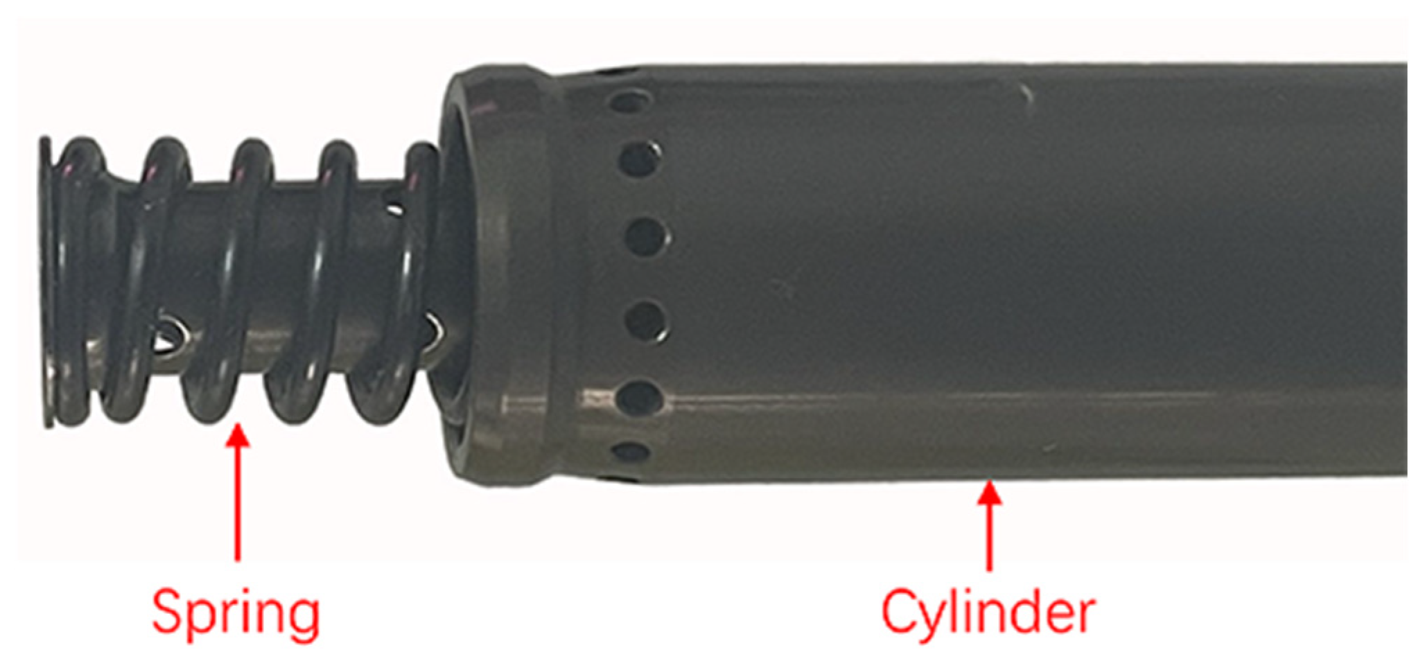
After analyzing the current situation of coaxiality measurement both domestically and abroad, it was found that the optical measurement technology proposed by researchers has been widely applied in the process of coaxiality measurement of parts. Although these measurement techniques boast high precision, they are not suitable for the coaxiality measurement of automobile brake piston components. As shown in Figure 1, due to the spring structure of the part itself, during a rotating movement the laser beam emitted by the laser sensor will sometimes irradiate inside the spring coils, and sometimes irradiate on the spring, which causes the laser sensor to fail to obtain accurate measurement values. Although capacitive sensors are widely used for displacement and angle measurements, their accuracy and sensitivity are relatively low. During the rotational motion of automobile brake piston components, the variation of the spring relative to the reference axis is very small, rendering capacitive sensors unable to provide accurate feedback information. Additionally, while coordinate measuring machines are high-precision instruments, they have low detection efficiency and high costs, and thus are unable to meet the automated testing needs of enterprises.
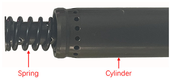
Figure 1.
Automobile brake piston component.
In recent years, with the rapid development of computer technology and wavelet analysis in the field of image processing and computer vision, many researchers have used machine vision technology to realize non-contact detection and online detection. Images can be decomposed into sub-images of different scales and frequencies by means of wavelet transform, and then edge detection, image denoising, and feature point extraction can be realized [10,11,12,13,14,15,16]. In addition, compared with traditional measurement technology, machine vision technology has high precision, high efficiency, and a low cost, and avoids the risk of damaging the surface of parts, so it has been widely studied [17,18,19,20,21]. Many researchers have studied shaft parts based on machine vision technology.
Li et al. [22] proposed a geometric measurement system for shaft parts based on machine vision. The system first utilized industrial cameras to capture images of the parts. Then, a series of image preprocessing algorithms were used to obtain the image edge contour. Finally, the image edge contour was measured via geometric algorithm, and thus the bottom radius of the cylinder contour and the height of the column were obtained. Zhang et al. [23] proposed a method for measuring the straightness, roundness and cylindricity of workpieces based on machine vision. A linear search algorithm and improved particle swarm optimization algorithm were proposed to evaluate the straightness and roundness deviation of workpieces. On this basis, a method to evaluate image cylindricity deviation using least squares fitting of circular center coordinates was studied. Wei et al. [24] proposed a measurement method of cylindrical shaft diameter based on machine vision. Sun et al. [25] proposed an axis diameter measurement method based on digital image processing technology. External parameters were calibrated by measuring the axis with known diameters, and new external parameters were used to improve measurement accuracy.
However, with regard to coaxiality measurement, related applications and relevant research are scarce. Therefore, aiming at addressing the problem of the online detection of automobile brake piston components, this paper proposes a non-contact coaxiality measurement method based on machine vision and digital image processing technology. In order to obtain real-time images of automobile brake piston components, an image acquisition system is designed. Through a written algorithm program, the precise extraction of the geometric feature points of automobile brake piston components is realized, which reduces the manual operation, improves detection efficiency and accuracy, and lays a foundation for the on-line detection of the coaxiality of the stepped shaft parts. The rest of this article is organized as follows: Section 2 describes in detail the detection principle, image preprocessing process, and the method of extracting geometric feature points. Section 3 analyzes and discusses the experimental results, potential future research areas, and the reproducibility and scalability of other shaft parts. Section 4 summarizes the conclusions of this study.
2. Detection Methods
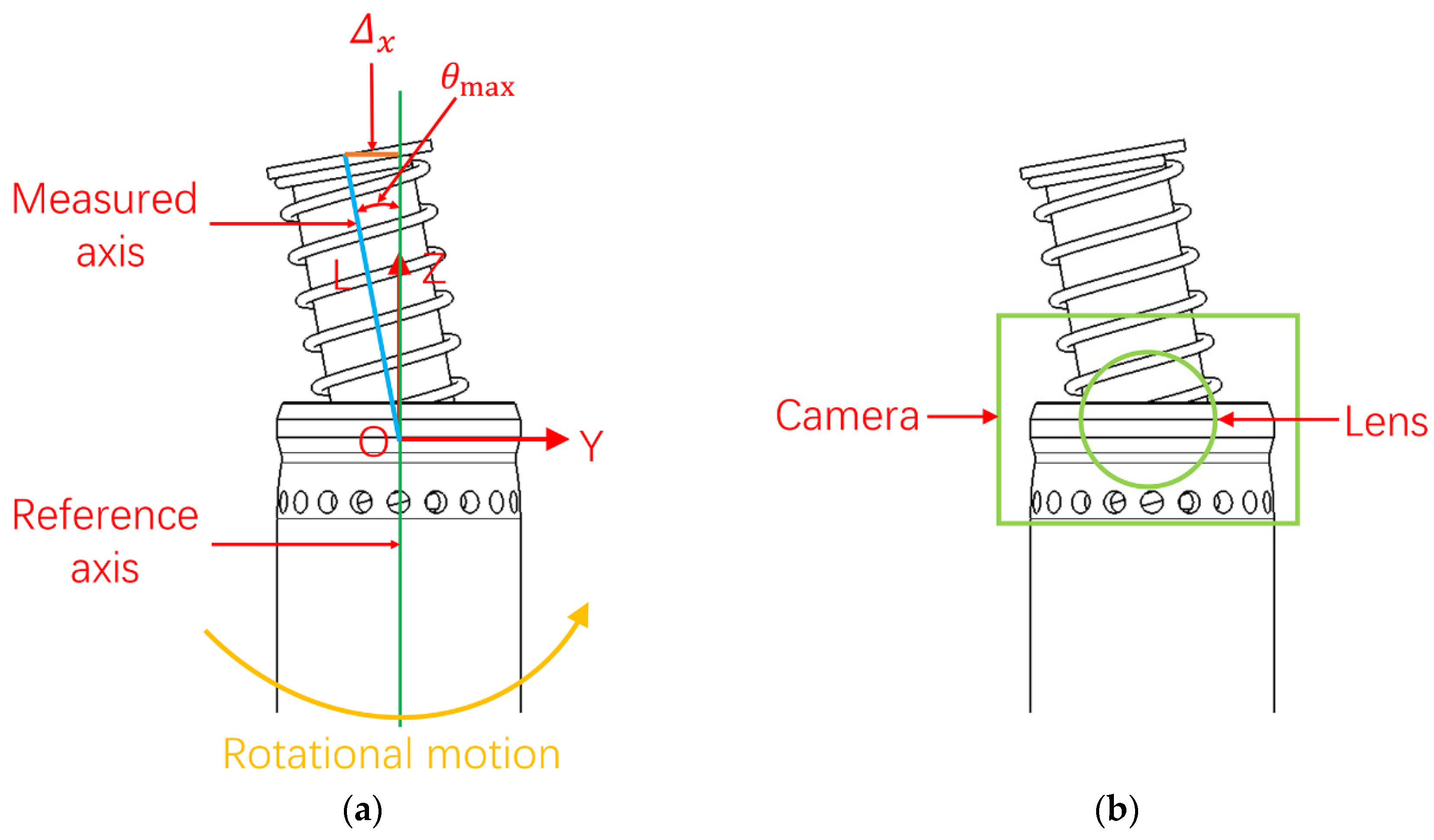
The coaxiality error can be understood as the maximum variation between two axis lines. Therefore, the key to calculating the coaxiality error value lies in obtaining the equations of the measured axis and the reference axis. During the assembly process of automobile brake piston components, inevitable assembly errors occur between the spring and the cylinder. This error causes a variation between the axis of the spring and the axis of the cylinder, which is denoted as θ.
The mathematical model of an automobile brake piston component is shown in Figure 2a. The blue line represents the axis of the spring (measured axis), while the green line represents the axis of the cylinder (reference axis). The origin of the coordinate system is at the junction between the spring and the cylinder, denoted as O, the coordinate system OXYZ is established, and the Z axis is the reference axis.
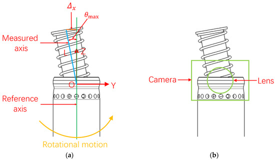
Figure 2.
Schematic diagram of the coaxiality detection principle: (a) the mathematical model; (b) the position relationship between the measured part and the industrial camera.
An industrial camera is positioned horizontally in front of the measured part (the position relationship between the industrial camera and the automotive brake piston component is shown in Figure 2b). During the rotation of the automobile brake piston component around the Z-axis, there is a moment when the blue axis is located exactly on the YOZ plane. At this time, the image captured by the industrial camera is the maximum variation of the spring part relative to the reference axis, denoted as . Moreover, the more images are collected, the closer the value of is to the real value. At this time, the distance between the center of the circle on the surface of the spring part and the reference axis is the coaxiality error, which is denoted as , and its mathematical calculation formula is as follows:
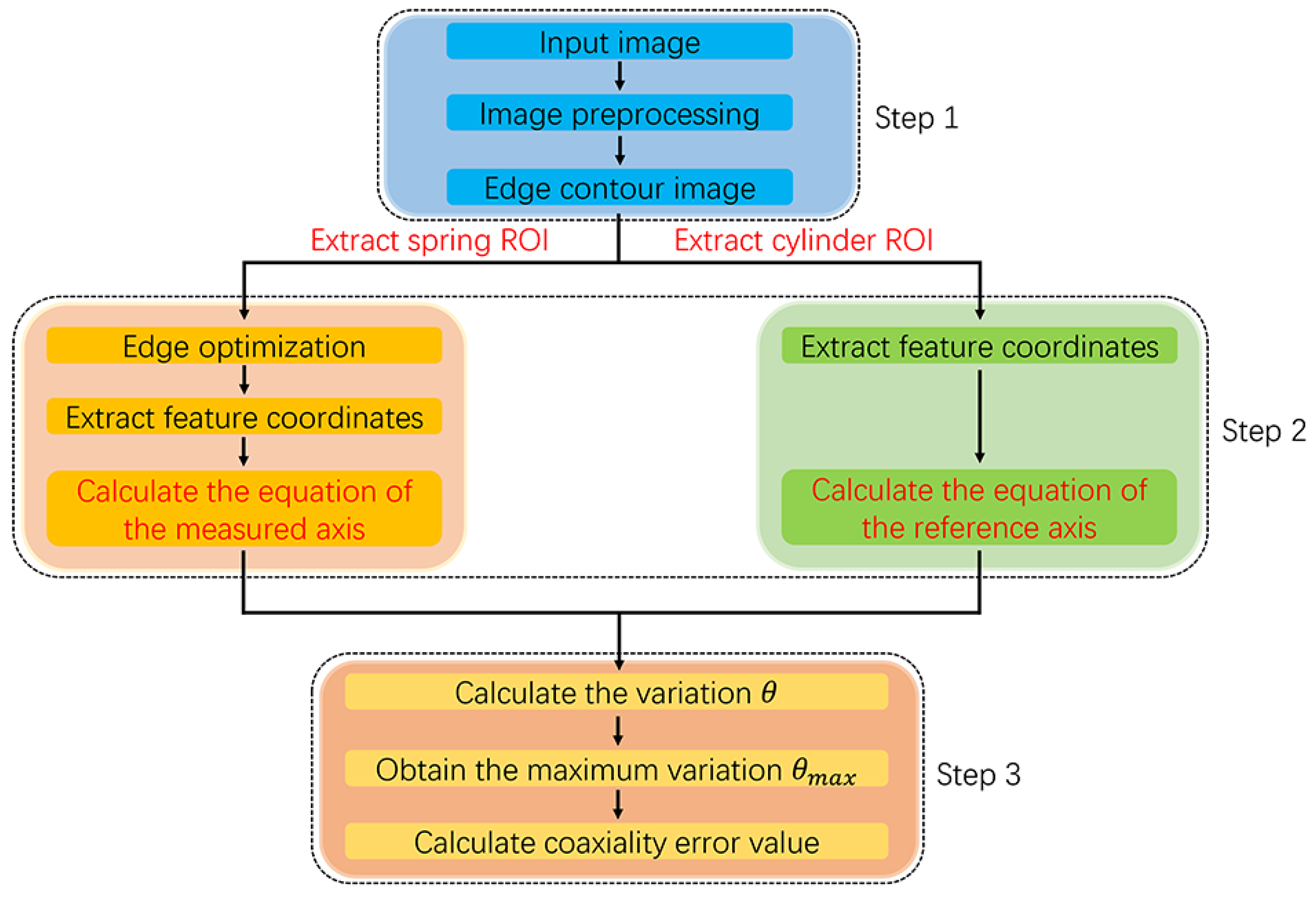
The flow chart of the detection method is shown in Figure 3. The first step is to obtain the edge contour of the unit pixel width of the target region through a series of image preprocessing algorithms, then extract the region of interest of the target region, and divide the automobile brake piston component into the spring ROI and the cylinder ROI. The second step is to optimize the edge of the region of interest of the spring, and then extract the geometric feature points of the two parts, so as to calculate the equation of the measured axis and the reference axis. The third step is to utilize the two equations obtained from the calculation, calculate the variation θ, and then extract the maximum variation among a series of images, so as to calculate the coaxiality error value.

Figure 3.
Flow chart of detection method.
2.1. Image Preprocessing
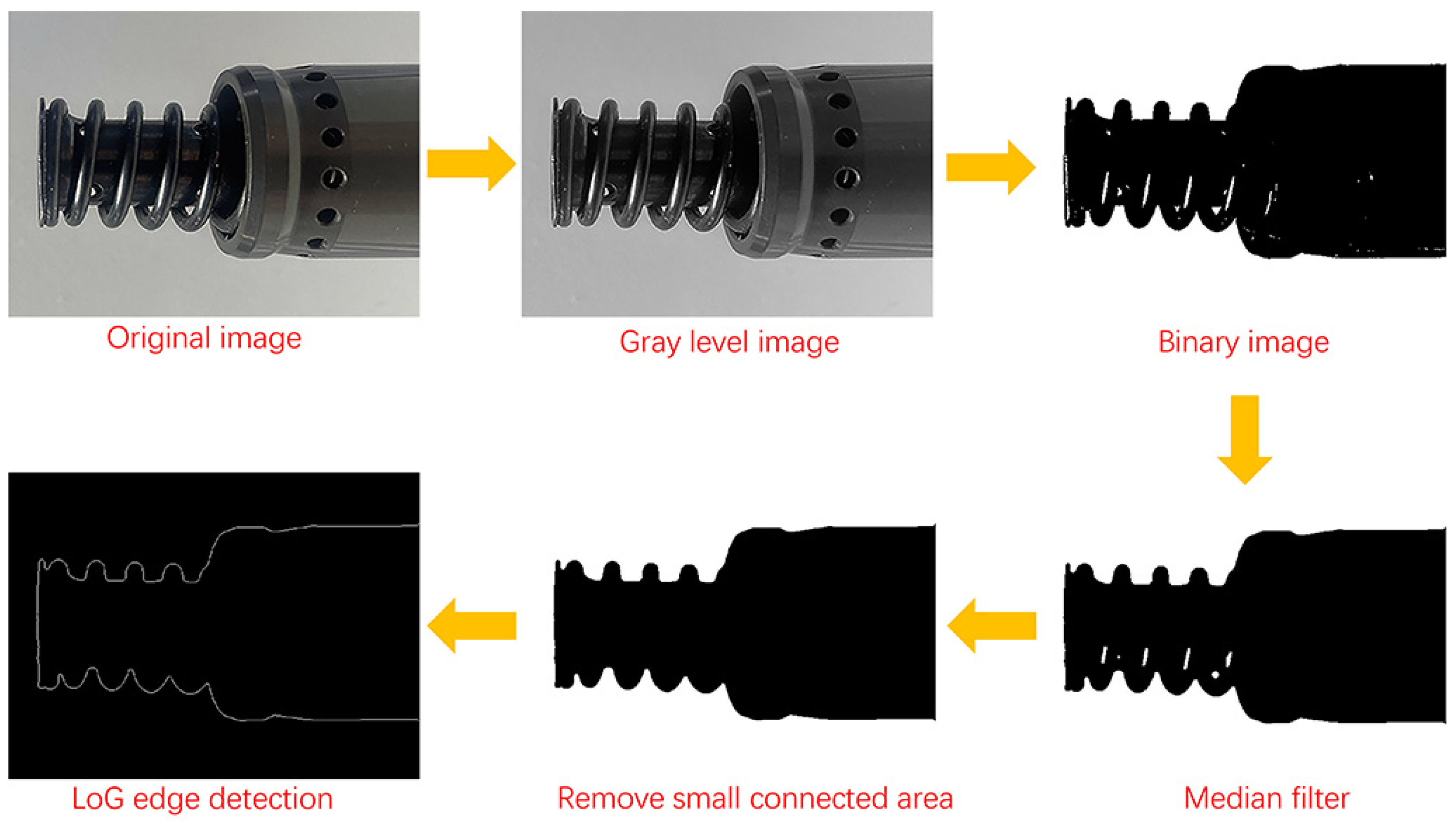
The flow chart of image preprocessing is shown in Figure 4. The image is captured using color industrial cameras, so the first step is to convert the color image to a gray image. The second step is image segmentation. The purpose of image segmentation is to separate the target region from the background region, so image segmentation holds a crucial position in image detection techniques. The gray image is defined as a two-dimensional function f(x,y), where the output of the function represents the grayscale value of a pixel point. The region of the target is dark colored while the background region is light colored. Based on this characteristic of the image, it is possible to find a suitable threshold value T to separate the target region from the background, thereby achieving binarization. Its mathematical expression is as follows:
where is the binarized image.
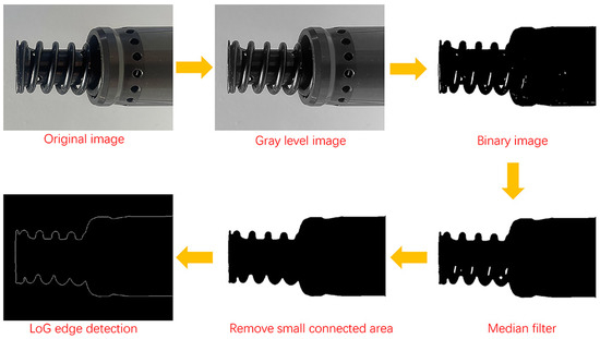
Figure 4.
Flow chart of image preprocessing.
During the image acquisition process, factors such as uneven lighting and electromagnetic interference can lead to the presence of a lot of noise in the image, which can significantly affect subsequent image processing. Because the median filter can remove noise while ensuring edge details, the effect is better, so we use the median filter [26]. After filtering and denoising, the image may still contain some small objects. The fourth step involves utilizing mathematical morphology techniques to remove small connected regions, thus obtaining a clean and clear target region. Compared to first-order differential operators, second-order differential operators can more accurately locate edges, and the obtained edge contour is basically the unit pixel width. Therefore, the Laplacian of Gaussian operator is used for edge detection in the final step.
2.2. Extract the Region of Interest
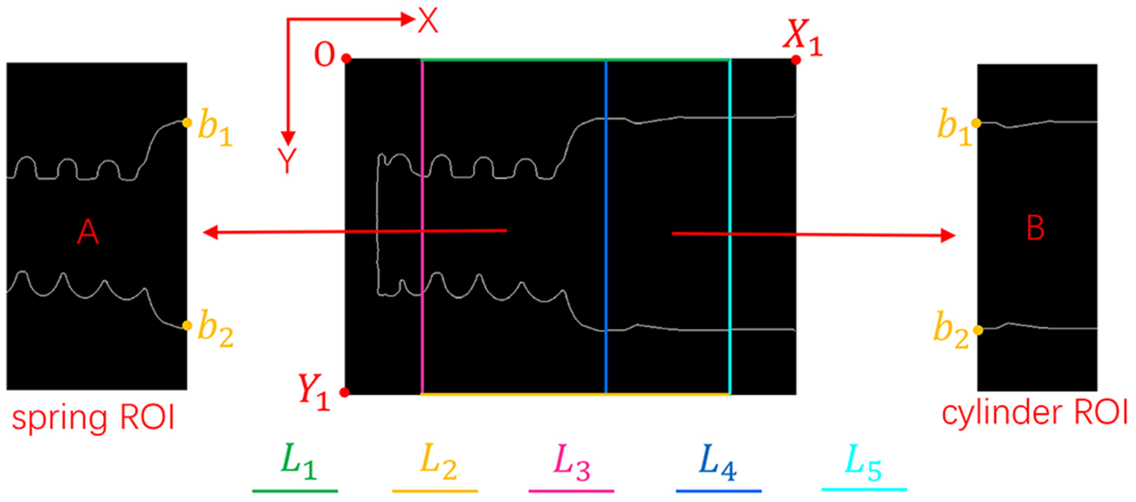
There are often many useless regions in the actual collected original image, which will cause adverse effects on the subsequent extraction of geometric feature points. Therefore, in order to facilitate the subsequent research, it is necessary to extract the effective region in the image. The extracted ROI region is shown in Figure 5.
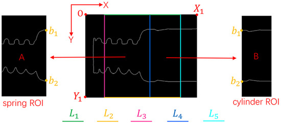
Figure 5.
Extraction of ROI region.
The contour of the target region was obtained via the Laplacian of Gaussian edge detection algorithm, as shown in Figure 5, setting it as F(x,y), width and height . The upper dividing line and lower dividing line in the horizontal direction of the region of interest correspond to the upper and lower edges of the image, so the equations for and are as follows:
The relationship between the left dividing line in the vertical direction and the image width is expressed as . The relationship between the middle dividing line in the vertical direction and the image width is expressed as . The relationship between the right dividing line in the vertical direction and the image width is expressed as ; , , and , are the constants used to adjust the ROI region size, and .
The rectangle formed by the four lines , , , and represents the spring ROI, denoted as region A, as shown in Figure 5. Region A can be calculated using Equation (4).
The rectangle formed by the four lines , , , and represents the cylinder ROI, denoted as region B, as shown in Figure 5. Region B can be calculated using Equation (5).
2.3. Extracting Geometric Feature Points of the Cylinder
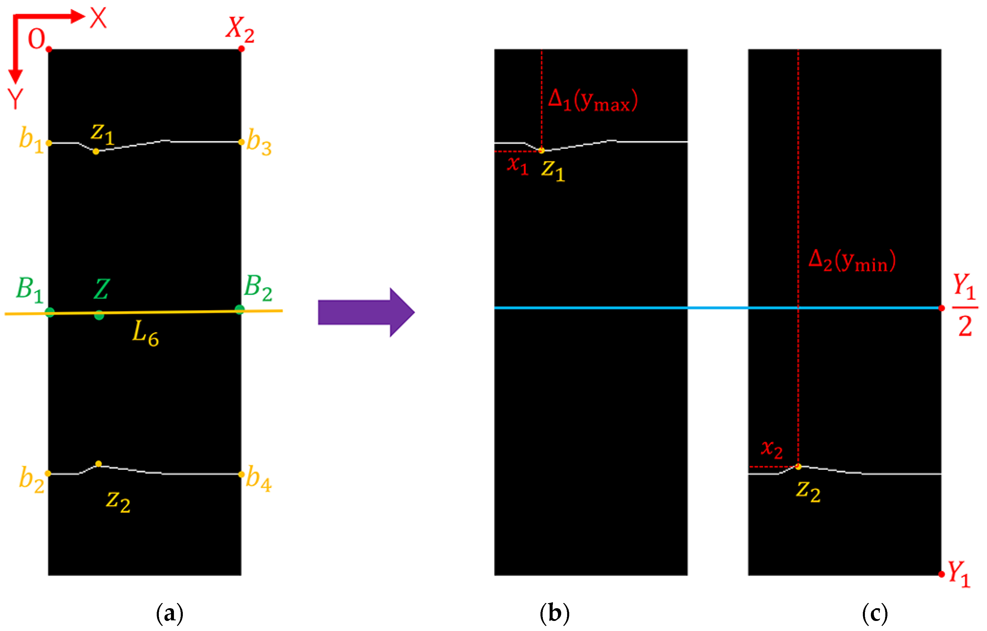
The structure of automobile brake piston components is complicated, and the geometric feature points of the upper and lower edges cannot be extracted at the same time, so the pixel points of the upper edge and lower edge need to be separated. The separation results of the pixel points on the upper and lower edges of the cylinder are shown in Figure 6. The schematic diagram illustrating the calculation of the reference axis equation is shown in Figure 6a. The region of interest of the cylinder is set as , the width is , and the height is .
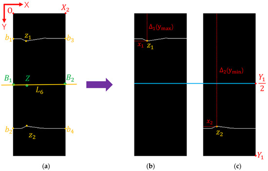
Figure 6.
The result of the separation of pixel points on the upper and lower edges of the cylinder: (a) schematic diagram of the calculation reference axis; (b) removing the lower edge pixel points; (c) removing the upper edge pixel points.
If we extract the pixel points where and store them in a new two-dimensional array , the mathematical expression for the pixel points on the upper and lower edge of the cylinder is as follows:
where represents the pixel points on the upper edge of the cylinder. represents the pixel points on the lower edge of the cylinder.
The image after removing the pixel points on the lower edge of the cylinder is shown in Figure 6b. The two-dimensional array has elements and can be regarded as an matrix, denoted as . The first row of matrix corresponds to the coordinates of , while the last row corresponds to the coordinates of . By extracting the first row of matrix , we obtain the coordinates of , denoted as . By extracting the last row of matrix , we obtain the coordinates of , denoted as . The image after removing the pixel points on the upper edge of the cylinder is shown in Figure 6c. The coordinates of and can be obtained by means of the same method as above, set as and .
As can be seen from the schematic diagram of extracting the extreme value points of the cylinder in Figure 7, there are multiple extreme points at the wave peak and wave trough positions, and the first pixel point is selected as the extreme point in this paper. The specific methods for extracting the coordinates of extreme points and are as follows:
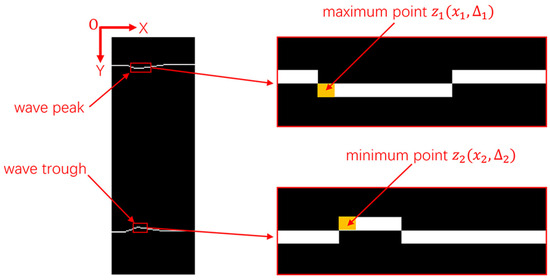
Figure 7.
Schematic diagram of extract cylinder extremum point.
- (1)
- Extract the y-elements from the two-dimensional array and store them in a new one-dimensional array. Find the largest element in this one-dimensional array. This maximum element corresponds to the y coordinate of and is denoted as .
- (2)
- Extract all elements from the two-dimensional array where , and store them in a new two-dimensional array . Extract the first element from . This element represents the coordinate value of the extremum point , denoted as , as shown in Figure 7.
- (3)
- Extract the y-elements from the two-dimensional array and store them in a new one-dimensional array. Find the minimum element in this one-dimensional array. This minimum element corresponds to the y coordinate of and is denoted as .
- (4)
- Extract all elements from the two-dimensional array where , and store them in a new two-dimensional array . Extract the first element from . This element represents the coordinate value of the extremum point , denoted as , as shown in Figure 7.
Because the coordinates of pixel points are discrete data, the coordinates must be integers.
Therefore, the coordinates of the midpoint between the extreme points and are ([( + )/2], [( + )/2]). The coordinates of the midpoint between and are (1, [(Y2 + Y3)/2]). The coordinates of the midpoint B2 between b3 and b4 are (X2, [(Y4 + Y5)/2]).
The coordinates of B1, Z and B2 are set as B1(U1 = 1, V1 = [(Y2 + Y3)/2]), Z(U2 = [(x1 + x2)/2], V2 = [( + )/2]), and B2(U3 = X2, V3 = [(Y4 + Y5)/2]). According to the principle of the least squares method [27,28,29,30], the equation of reference axis L6 can be obtained via the linear fitting of B1, Z and B2, and the slope of reference axis L6 is denoted as K1, as shown in Equation (7) as follows:
In Formula (7), represents the intercept of the fitted line.
2.4. Edge Optimization
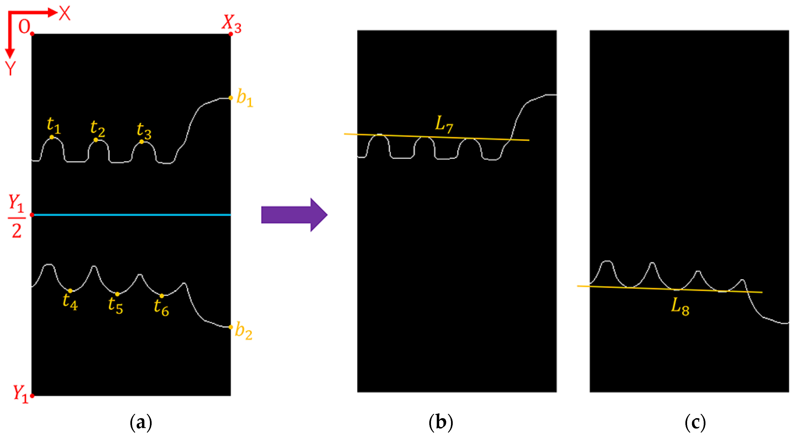
The process of separating the upper and lower edge pixel points of the spring is the same as the process of separating the upper and lower edge pixel points of the cylinder. A schematic diagram of the separation process is shown in Figure 8a. The image after removing the lower edge pixel points is shown in Figure 8b. The image after removing the upper edge pixel points is shown in Figure 8c.
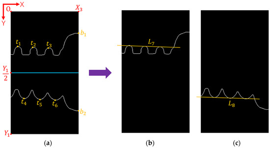
Figure 8.
The result of the separation of pixels on the upper and lower edges of the spring: (a) schematic diagram of the separation process; (b) removing the lower edge pixel points; (c) removing the upper edge pixel points.
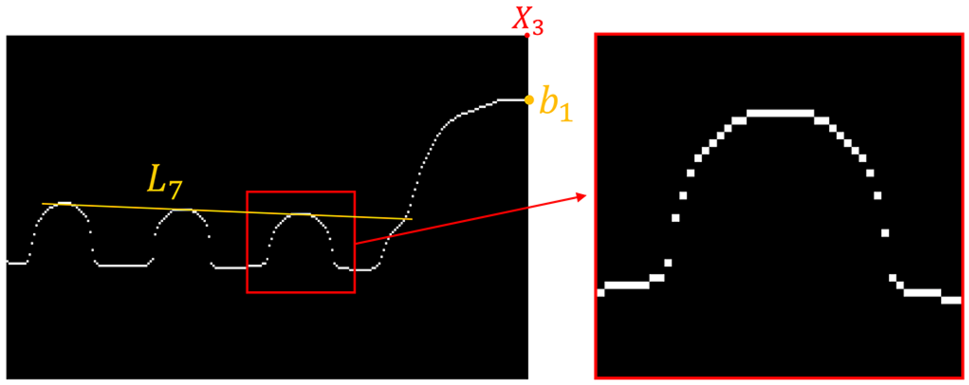
Figure 9 shows the upper edge of the spring before optimization. It can be observed that each column in the image typically contains multiple pixel points. These extra pixel points can interfere with the subsequent extraction of geometric feature points. Therefore, the upper edge of the spring needs to be optimized so that each column has only one pixel point. The specific optimization process is as follows.
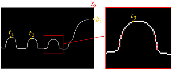
Figure 9.
Before edge optimization.
- (1)
- As shown in Figure 8b, the image after removing the lower edge pixel points of the spring is set to Ts(x,y) and the width is X3. The spring edge pixel points of each column in the image Ts(x,y) are extracted successively, and X3 two-dimensional arrays E(x,y) are obtained.
- (2)
- The first element in the two-dimensional array E(x,y) is extracted and stored in a new two-dimensional array E1(x,y), and X3 pixels on the upper edge of the spring are obtained. The optimized results are shown in Figure 10.
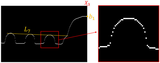 Figure 10. After edge optimization.
2.5. Extracting Geometric Feature Points of the Spring
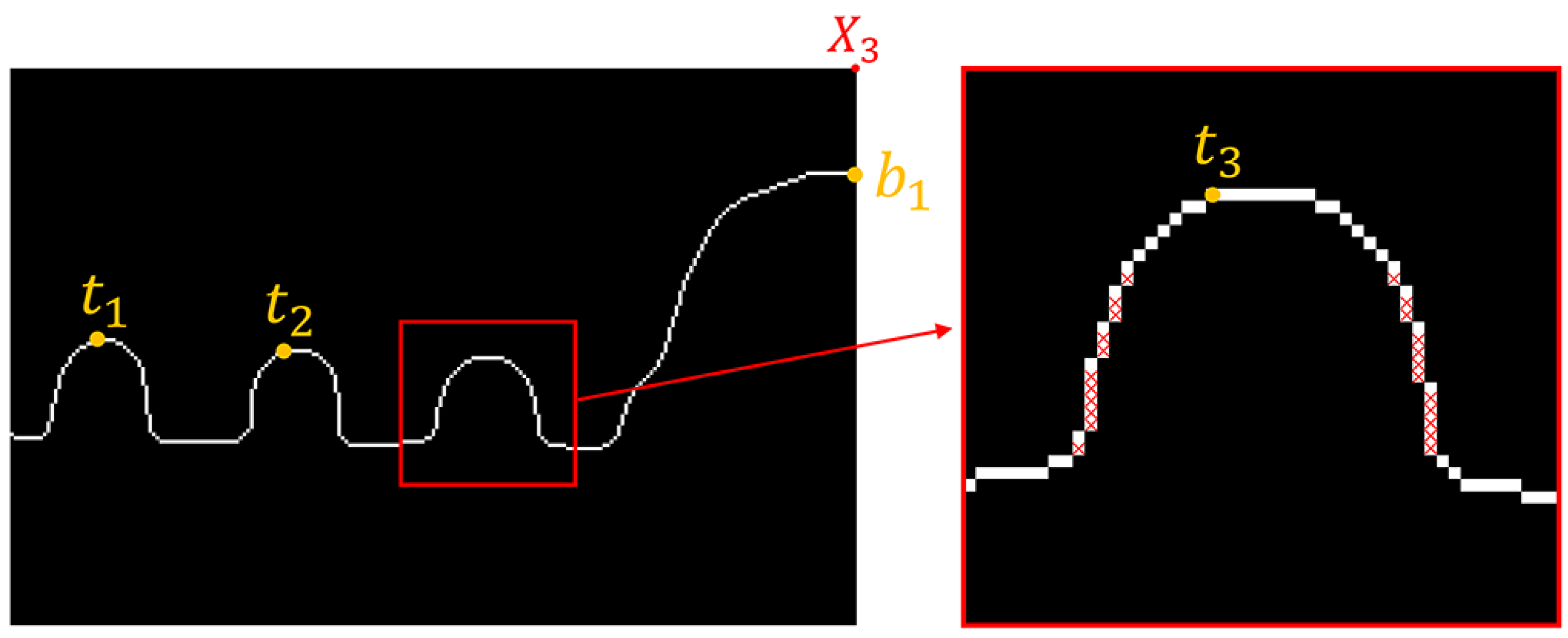
As shown in Figure 11, the geometric feature points on the upper edge of the spring are located at the wave trough positions. Therefore, it is necessary to extract all the wave trough pixel points on the upper edge of the spring.

Figure 11.
Schematic diagram of geometric feature points of the spring.
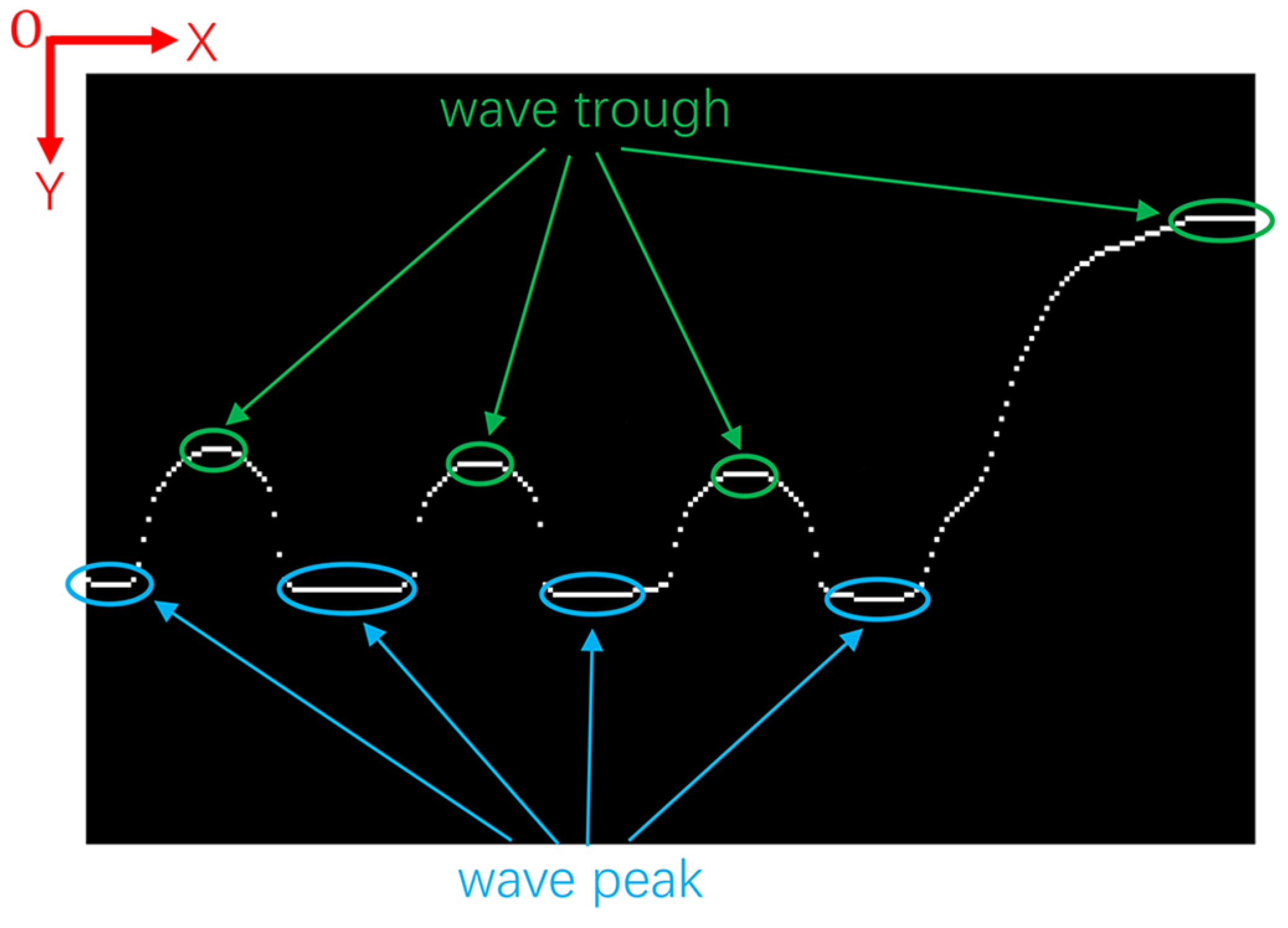
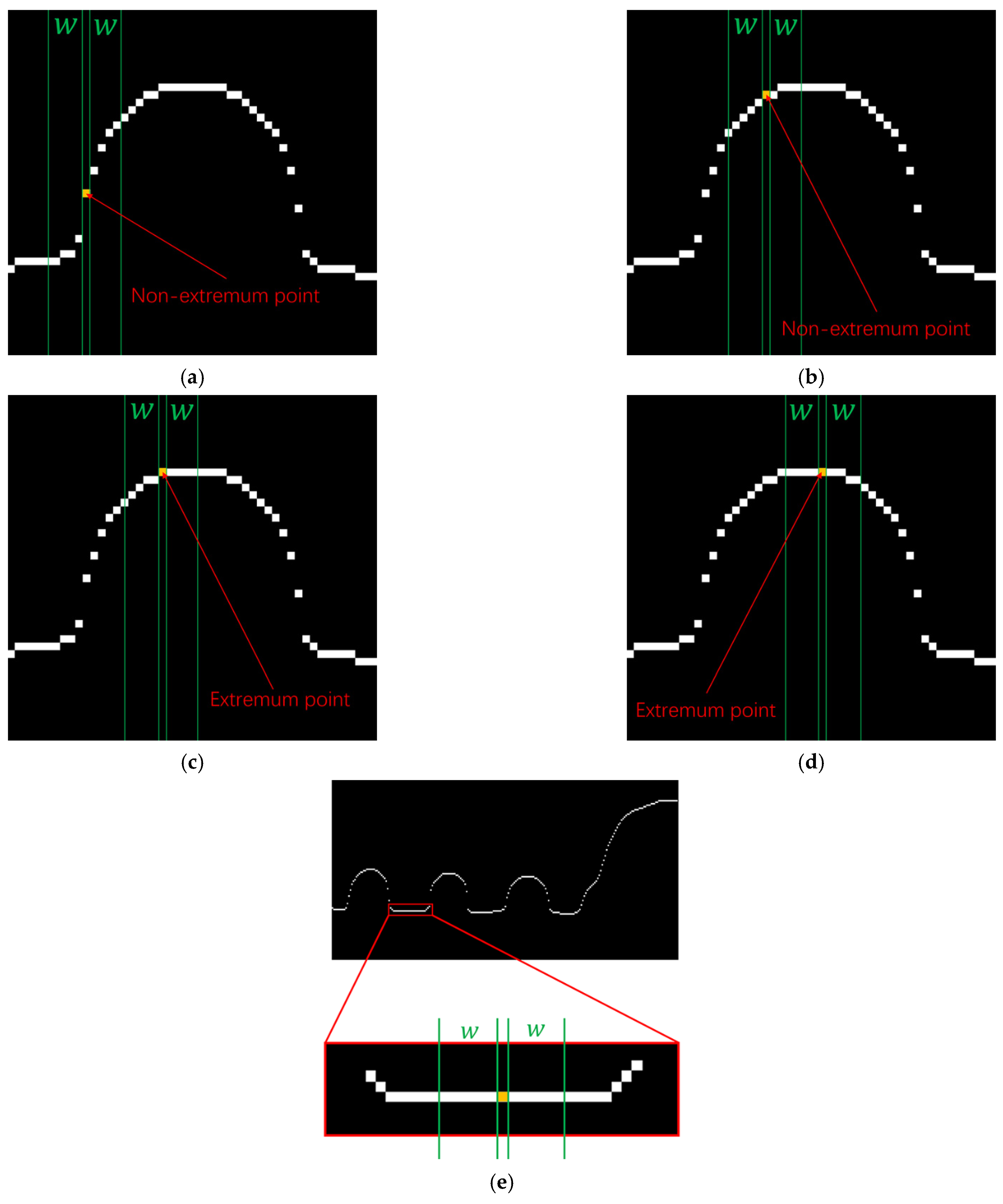
The principle of extracting extremum points of the wave trough is illustrated in Figure 12. The specific steps are as follows:
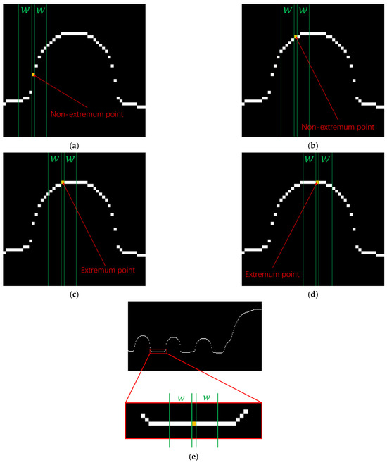
Figure 12.
Principle of extracting wave trough pixel points: (a) non-extreme point; (b) non-extreme point; (c) extremum point; (d) extremum point; (e) extract wave peak extremum points.
- (1)
- Given a neighborhood interval centered around a pixel point, the neighborhood radius includes pixel points.
- (2)
- Start from the leftmost pixel point of the image and go through all the pixel points in the image in turn.
- (3)
- If the y-value of the pixel point is less than or equal to the y-values of the pixel points within the neighborhood, that pixel point is a extremum point, and stored in a new two-dimensional array. This process results in four new two-dimensional arrays.
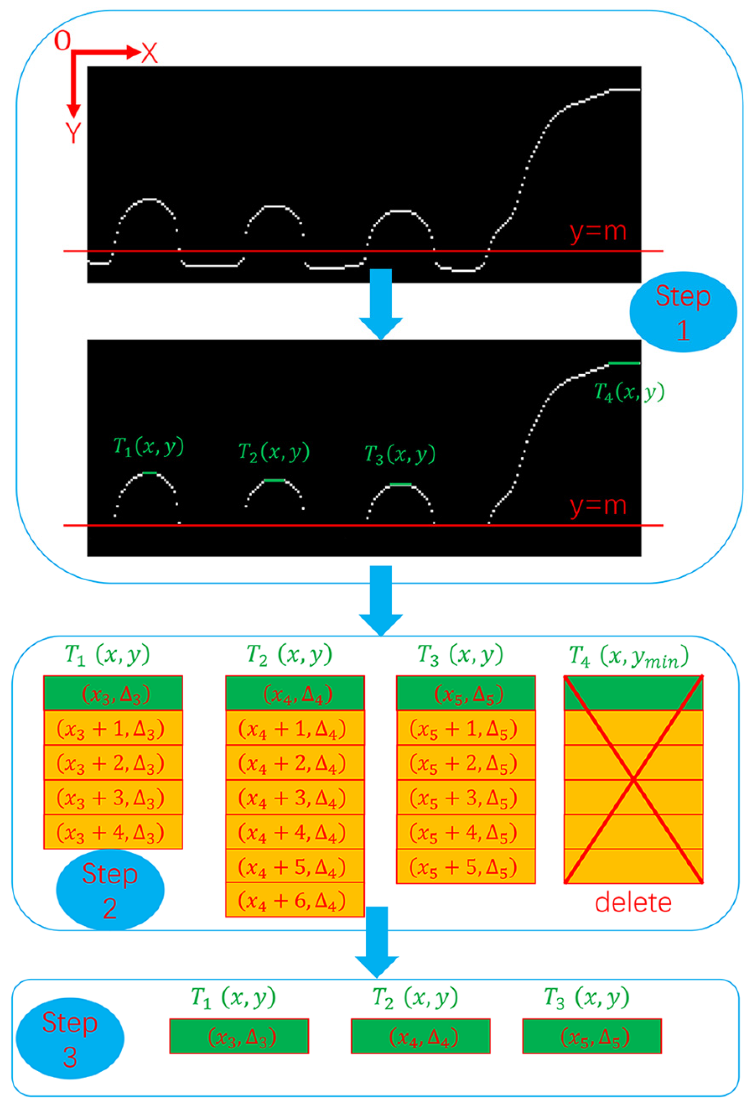
The process of extracting the coordinates of the three extreme points , , and on the upper edge of the spring is shown in Figure 13. The specific steps are as follows:
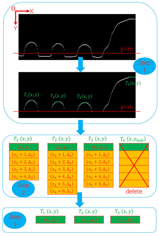
Figure 13.
Flow chart of extracting spring geometric feature points.
- (1)
- To further refine step 2, as mentioned earlier, there may be a situation where wave peak extremum points are extracted, as shown in Figure 12e. To avoid the impact of this situation on the results, the method in this paper involves setting a straight line before extracting wave trough extremum points and removing all pixel points where . The resulting image after this step is denoted as step 1 in Figure 13.
- (2)
- For the four two-dimensional arrays obtained from step 3 as described above, let them be denoted as T1(x,y), T2(x,y), T3(x,y) and T4(x,y).
- (3)
- It can be seen that the two-dimensional array T4(x,y) does not contain spring geometric feature points, and the y value in T4(x,y) is the minimum value. According to this condition, the two-dimensional array T4(x,y) can be deleted.
- (4)
- Extract the first element from T1(x,y), T2(x,y), and T3(x,y), which are the coordinates of the three extreme points t1, t2, t3, denoted as .
The coordinates of , , and are set as t1(U4 = x3, V4 = Δ3), t2(U5 = x4, V5 = Δ4), and t3(U6 = x5, V6 = Δ5). The equation of the tangential line L7 on the upper edge of the spring is fitted from Equation (7), and the slope and intercept of the line L7 are denoted as K2 and M2, so the equation of the tangential line L7 on the upper edge of the spring is y = K2·x + M2.
Using the same method as described above, we extract the geometric feature points on the lower edge of the spring, denoted as ,,.
The coordinates of , and are set as t4(U7 = x6, V7 = Δ6), t5(U8 = x7, V8 = Δ7), and t6(U9 = x8, V9 = Δ8). The equation of the tangential line L8 on the lower edge of the spring is fitted from Equation (7), and the slope and intercept of the line L8 are denoted as K3 and M3, respectively, so the equation of the tangential line L8 on the lower edge of the spring is y = K3·x + M3.
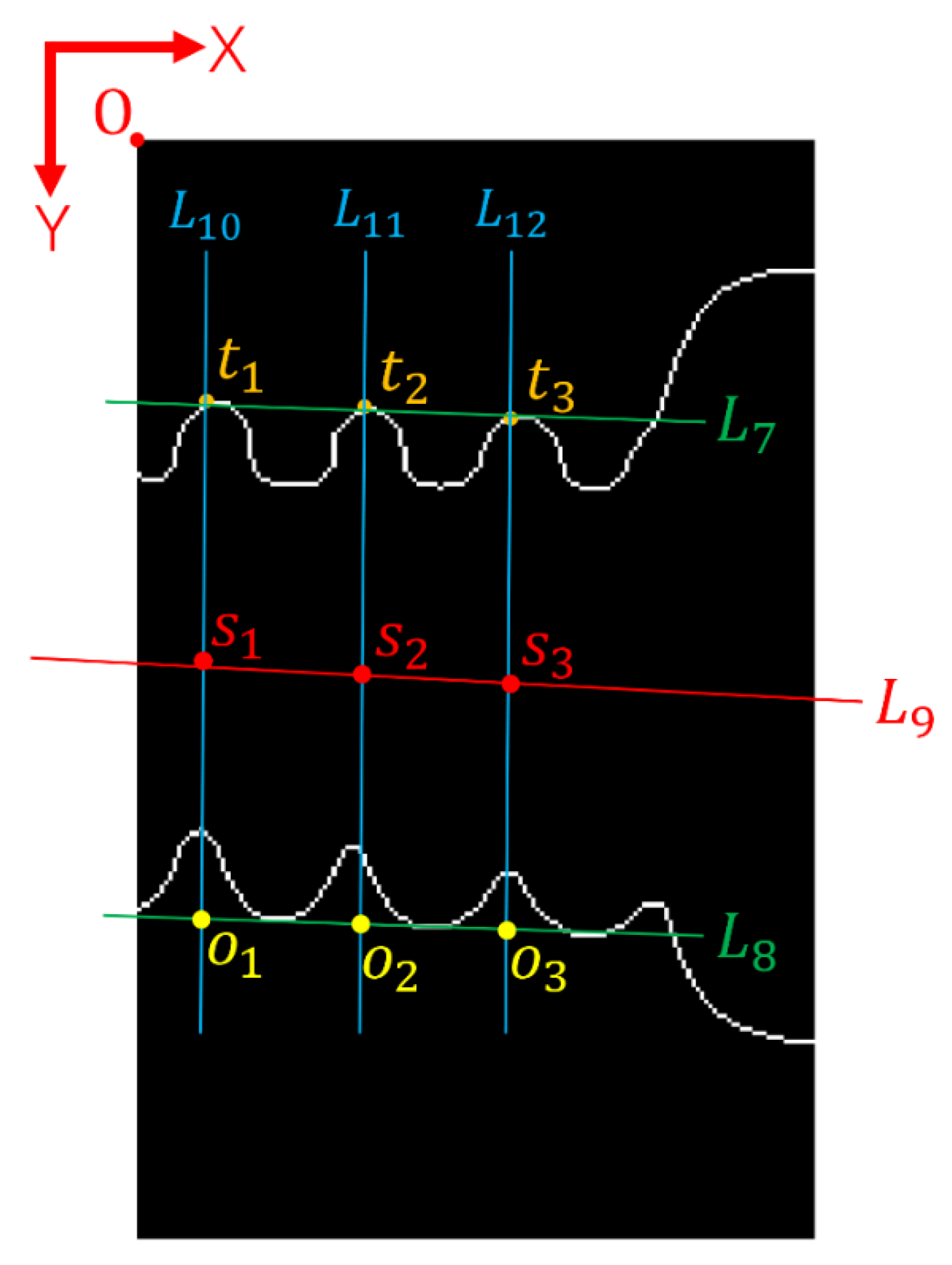
2.6. Calculate the Equation of the Measured Axis
The measured axis in this study refers to the axis of the spring. The schematic diagram of calculating the measured axis is shown in Figure 14. The specific calculation process is as follows:
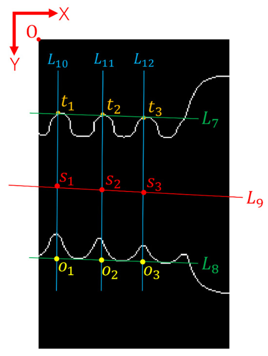
Figure 14.
Schematic diagram for calculating the measured axis.
- (1)
- Given three straight lines in the vertical direction, the three straight lines pass the extreme points t1, t2 and t3 on the upper edge of the spring, respectively. Because the three extreme value point coordinate values are t1(x3, Δ3), t2(x4, Δ4), and t3(x5, Δ5), the equation of three lines is L10: x = x3, L11: x = x4, and L12: x = x5, respectively.
- (2)
- The three points where the three straight lines intersect the tangent line L8 of the lower edge of the spring are set as o1, o2, and o3, respectively. Because the equation of line L8 is y = K3·x + M3, the coordinates of the three intersection points are o1 (x3, K3·x3 + M3), o2 (x4, K3·x4 + M3), and o3 (x5, K3·x5 + M3), respectively.
- (3)
- The coordinates of s1, s2, and s3 can be determined as s1(x3, [(Δ3 + K3·x3 + M3)/2]), s2(x4, [(Δ4 + K3·x4 + M3)/2]), and s3(x5, [(Δ5 + K3·x5 + M3)/2]), respectively.
- (4)
- The coordinates of s1, s2 and s3 are set as s1(U10 = x3, V10 = [(Δ3 + K3·x3 + M3)/2]), s2(U11 = x4, V11 = [(Δ4 + K3·x4 + M3)/2]), and s3(U12 = x5, V12 = [(Δ5 + K3·x5 + M3)/2]), respectively.
- (5)
- The equation of the measured axis L9 can be fitted from Equation (7), and the slope of the measured axis L9 is denoted as K4. The angle θ between the measured axis L9 and the reference axis L6 can be calculated using Equation (8).
3. Experimental Verification
3.1. Detection System
To validate the feasibility and accuracy of the proposed algorithm in this paper, we conducted a coaxiality simulation experiment. According to the experimental requirements, a coaxiality detection system was designed, as shown in Figure 15. The detection system mainly consisted of an electric rotary platform, an industrial camera, a lens, an LED ring light source, a stepper motor driver and controller, and a computer, among other components.
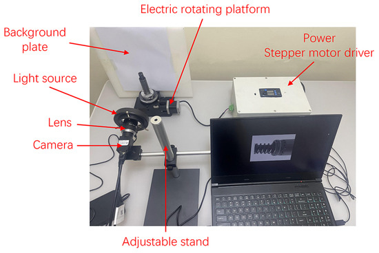
Figure 15.
Detection system.
The industrial camera used in the experiment was the Hikvision MV-CU120-10GC color CMOS array camera (Industrial Camera and Lens Sourcing with Changchun, China), with a resolution of 3036 pixels × 4024 pixels. The lens was the Hikvision MVL-KF5028M-12MP, which is a high-definition, ultra-low distortion lens. The light source was an LED ring light with a diameter of 100 mm, and its brightness was adjustable.
The electric rotating platform drove the measured part to perform rotational motion, and the driver sent pulse signals to the stepper motor, which was set to rotate 9°, pause for 0.5 s, and repeat 40 times. A total of 40 images were collected.
3.2. Experimental Results
The 40 captured images were input into the computer, and the angles θ between the spring axis and the reference axis were calculated using the algorithm proposed in this paper. The results are shown in Table 1. From the detection results, it can be seen that the angles from the 1st to the 24th image show an increasing trend, with the angle being maximum for the 25th image. The angles from the 26th to the 40th image show a decreasing trend. The variation in angle conforms to objective rules, further proving the feasibility and correctness of the detection method proposed in this paper.

Table 1.
Angle θ between spring axis and datum axis of 40 images.
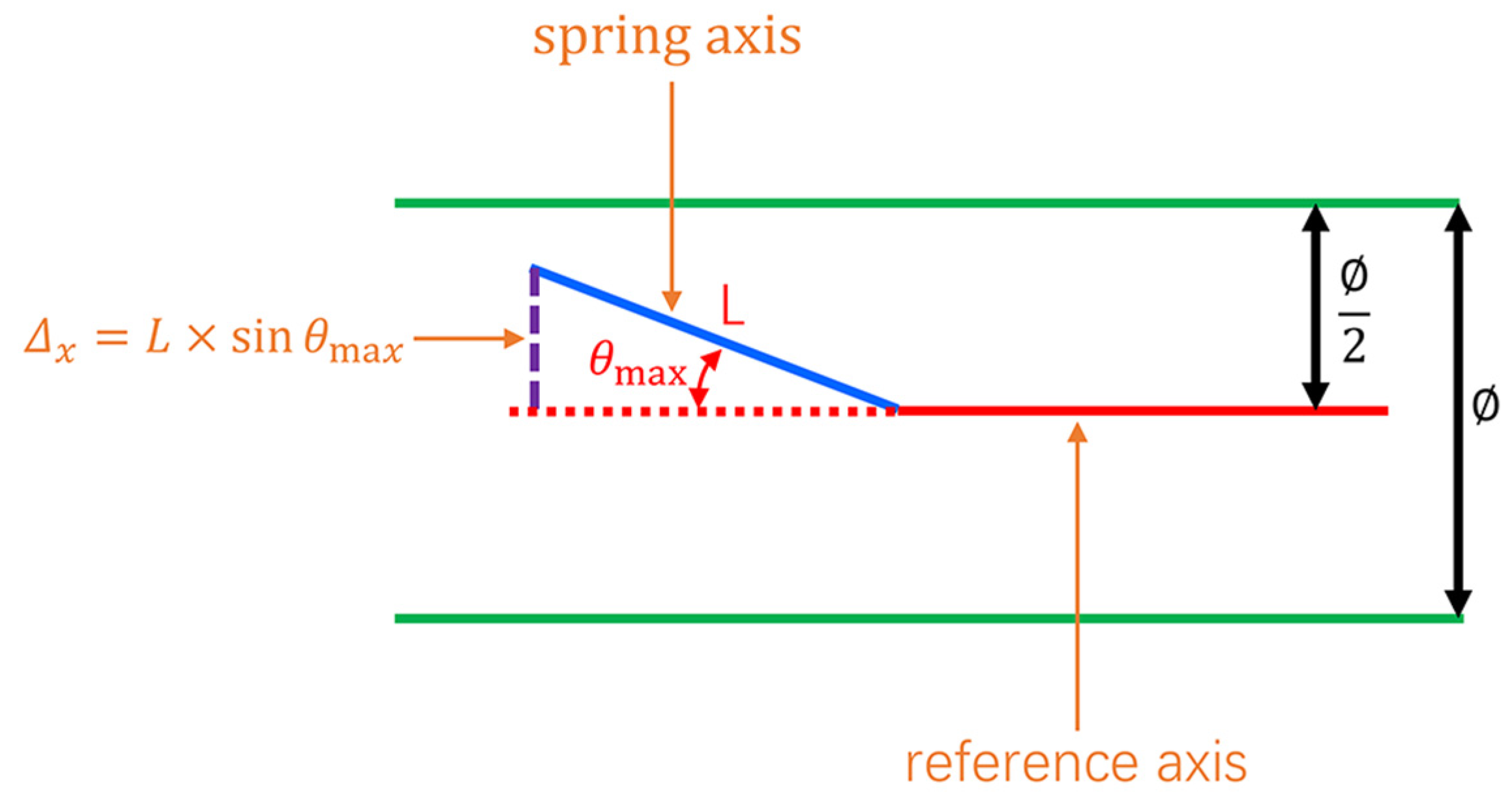
Taking the maximum angle of 1.0254° from the 40 images as the maximum variation of the spring relative to the reference axis, the coaxiality error could be calculated using Equation (1). The calculated result met the requirements of coaxiality tolerance. The delivery inspection report of the measured part is a qualified product, which proves the feasibility of the detection method in engineering practice, and the coaxiality evaluation schematic is shown in Figure 16.
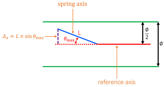
Figure 16.
Schematic diagram of evaluation coaxiality.
To further validate the stability of the algorithm proposed in this paper, we conducted coaxiality testing on ten automotive brake piston components. Among them, seven were qualified products and three were unqualified. The results of the testing using the algorithm proposed in this paper were consistent with the delivery inspection reports of the measured parts. A total of 400 images were obtained for the ten automotive brake piston components, with three images failing to extract geometric feature points, resulting in a success rate of 99.25%. This further demonstrates that the detection method proposed in this paper meets the online detection requirements for automobile brake piston components.
3.3. Discussion and Analysis
In the testing results, three images failed to extract geometric feature points due to minor changes in lighting, resulting in poor binary image quality and subsequently affecting the extraction of geometric feature points. To avoid this situation, it is recommended to install a darkroom on the production line to provide sufficient and stable lighting. Many researchers have studied coaxiality detection, and our proposed method was compared with those of other researchers, as shown in Table 2. Currently, the main methods involve using laser displacement sensors and laser alignment. However, most of the methods of other researchers are only suitable for the detection of a certain part. In this paper, only the coaxiality measurement of automobile brake piston components in a certain braking system was carried out. The proposed measurement method, by modifying the algorithm parameters and extracting the required geometric feature points, can be fully extended to the coaxiality measurement of other stepped shaft parts, such as the motor shaft, gear shaft and guide shaft, which will be the focus the author’ future research work. Therefore, the novelty of this measurement method lies in its flexibility and accuracy.
Table 2.
Comparison with other researchers’ detection methods.
4. Conclusions
This study implemented the detection of coaxiality for automotive brake piston components based on machine vision and image processing technology. The novelty of the proposed detection method lies in its accuracy and flexibility. The theory and experiment show that the accuracy and stability of the method can reach 99.25%, and the coaxiality of other stepped shaft parts can be measured by modifying the algorithm parameters, meeting the requirements of automated detection in enterprise. This method has advantages such as high precision, efficiency, and stable performance, showing promising application prospects and laying a foundation for online coaxiality detection of automotive brake piston components. Additionally, this research outcome provides a new method for coaxiality detection of similar parts to stepped shafts. The main contributions of this paper are as follows:
- Analyzing the structural characteristics of automotive brake piston components and extracting the regions of interest based on these characteristics.
- Proposing a mathematical morphology-based edge optimization method for complex edge structures, which removes redundant pixel points and optimizes image data into an n × n matrix (where n is the width of the image), thereby improving the accuracy of geometric feature point extraction.
- Determining the positions of extreme points by comparing the height of pixel points with that of neighboring pixel points, thus successfully extracting the coordinates of geometric feature points.
In summary, the non-contact detection method based on the integration of machine vision and image processing technology offers an effective solution for the online detection of coaxiality in automobile brake piston components, demonstrating practicality and feasibility. However, there is still room for further optimization and improvement to adapt to evolving production demands and technological advancements. As a future research agenda, continuous experimental validation will be considered to ensure the method’s viability and stability under various conditions. Additionally, ongoing refinement and optimization of the approach will be pursued to accommodate diverse production environments and process requirements.
Author Contributions
Q.L.: research ideas, experimental design and data analysis; W.G.: writing manuscripts, charting, data collection, literature retrieval; H.S.: data collection, data analysis, literature retrieval; W.Z.: document retrieval, data collection, data analysis; S.Z.: experimental design, data collection, data analysis. All authors have read and agreed to the published version of the manuscript.
Funding
We need to thank the following organization for its strong support: the Natural Science Foundation of Jilin Province—General Project, 20220201043GX.
Institutional Review Board Statement
Not applicable.
Informed Consent Statement
Not applicable.
Data Availability Statement
The data presented in this study are available on request from the corresponding author. The data are not publicly available due to privacy.
Acknowledgments
The authors would like to thank the members of the project team for their dedication and effort, and the teachers and schools for their help.
Conflicts of Interest
The authors declare no conflicts of interest.
References
- Xiao, Y.; Luo, Y.; Xin, Y.P.; Wang, X.D. Part Coaxiality Detection Based on Polynomial Interpolation Subpixel Edge Detection Algorithm. In Proceedings of the 3rd World Conference on Mechanical Engineering and Intelligent Manufacturing (WCMEIM), Shanghai, China, 4–6 December 2020; pp. 377–380. [Google Scholar]
- Liu, Y.M.; Wang, D.W.; Li, Z.K.; Bai, Y.; Sun, C.Z.; Tan, J.B. A coaxiality measurement method by using three capacitive sensors. Precis. Eng.-J. Int. Soc. Precis. Eng. Nanotechnol. 2019, 55, 127–136. [Google Scholar] [CrossRef]
- Dou, Y.P.; Zheng, S.; Ren, H.R.; Gu, X.H.; Sui, W.T. Research on the measurement method of crankshaft coaxiality error based on three-dimensional point cloud. Meas. Sci. Technol. 2024, 35, 035202. [Google Scholar] [CrossRef]
- Chai, Z.; Lu, Y.H.; Li, X.Y.; Cai, G.; Tan, J.; Ye, Z.B. Non-contact measurement method of coaxiality for the compound gear shaft composed of bevel gear and spline. Measurement 2021, 168, 108453. [Google Scholar] [CrossRef]
- Wang, L.; Yang, T.Y.; Wang, Z.; Ji, Y.C.; Liu, C.J.; Fu, L.H. Simple measuring rod method for the coaxiality of serial holes. Rev. Sci. Instrum. 2017, 88, 113110. [Google Scholar] [CrossRef]
- Zhang, Y.G.; Wang, Y.D.; Liu, Y.J.; Lv, D.P.; Fu, X.B.; Zhang, Y.C.; Li, J.M. A concentricity measurement method for large forgings based on laser ranging principle. Measurement 2019, 147, 106838. [Google Scholar] [CrossRef]
- Gao, C.; Lu, Y.H.; Lu, Z.W.; Liu, X.Y.; Zhang, J.H. Research on coaxiality measurement system of large-span small-hole system based on laser collimation. Measurement 2022, 191, 110765. [Google Scholar] [CrossRef]
- Li, C.F.; Xu, X.P.; Sun, H.Q.; Miao, J.W.; Ren, Z. Coaxiality of Stepped Shaft Measurement Using the Structured Light Vision. Math. Probl. Eng. 2021, 2021, 5575152. [Google Scholar] [CrossRef]
- Zheng, Y.S.; Lou, Z.F.; Li, Y.; Wang, X.D.; Wang, Y. A Measuring Method of Coaxiality Errors for Apart Axis. In Proceedings of the 10th International Symposium on Precision Engineering Measurements and Instrumentation (ISPEMI), Kunming, China, 8–10 August 2018. [Google Scholar]
- Berry, M.V.; Lewis, Z.; Nye, J.F.J.P.o.t.R.S.o.L.A.M.; Sciences, P. On the Weierstrass-Mandelbrot fractal function. Proc. R. Soc. Lond. A Math. Phys. Sci. 1980, 370, 459–484. [Google Scholar]
- Guariglia, E. Harmonic Sierpinski Gasket and Applications. Entropy 2018, 20, 714. [Google Scholar] [CrossRef] [PubMed]
- Guariglia, E.; Guido, R.C. Chebyshev Wavelet Analysis. J. Funct. Spaces 2022, 2022, 5542054. [Google Scholar] [CrossRef]
- Guariglia, E.; Silvestrov, S. Fractional-Wavelet Analysis of Positive definite Distributions and Wavelets on D’(C). In Engineering Mathematics Ii: Algebraic, Stochastic and Analysis Structures for Networks, Data Classification and Optimization; Silvestrov, S., Rancic, M., Eds.; Springer Proceedings in Mathematics & Statistics; Springer: Berlin/Heidelberg, Germany, 2016; Volume 179, pp. 337–353. [Google Scholar]
- Guido, R.C.; Pedroso, F.; Contreras, R.C.; Rodrigues, L.C.; Guariglia, E.; Neto, J.S. Introducing the Discrete Path Transform (DPT) and its applications in signal analysis, artefact removal, and spoken word recognition. Digit. Signal Process. 2021, 117, 103158. [Google Scholar] [CrossRef]
- Yang, L.; Su, H.L.; Zhong, C.; Meng, Z.Q.; Luo, H.W.; Li, X.C.; Tang, Y.Y.; Lu, Y. Hyperspectral image classification using wavelet transform-based smooth ordering. Int. J. Wavelets Multiresolution Inf. Process. 2019, 17, 1950050. [Google Scholar] [CrossRef]
- Zheng, X.W.; Tang, Y.Y.; Zhou, J.T. A Framework of Adaptive Multiscale Wavelet Decomposition for Signals on Undirected Graphs. IEEE Trans. Signal Process. 2019, 67, 1696–1711. [Google Scholar] [CrossRef]
- Tan, Q.C.; Kou, Y.; Miao, J.W.; Liu, S.Y.; Chai, B.S. A Model of Diameter Measurement Based on the Machine Vision. Symmetry 2021, 13, 187. [Google Scholar] [CrossRef]
- Wu, X.F.; Wang, C.S.; Tian, Z.Z.; Huang, X.K.; Wang, Q. Research on Belt Deviation Fault Detection Technology of Belt Conveyors Based on Machine Vision. Machines 2023, 11, 1039. [Google Scholar] [CrossRef]
- Xiao, G.F.; Li, Y.T.; Xia, Q.X.; Cheng, X.Q.; Chen, W.P. Research on the on-line dimensional accuracy measurement method of conical spun workpieces based on machine vision technology. Measurement 2019, 148, 106881. [Google Scholar] [CrossRef]
- Ye, J.W.; Zhao, L.H.; Liu, S.; Wu, P.W.; Cai, J.T. Design and Experimentation of a Residual-Input Tube-End Cutting System for Plasma Bags Based on Machine Vision. Appl. Sci. 2023, 13, 5792. [Google Scholar] [CrossRef]
- Zhang, N.; Li, F.; Zhang, E.X. The Machine Vision Dial Automatic Drawing System-Based on CAXA Secondary Development. Appl. Sci. 2023, 13, 7365. [Google Scholar] [CrossRef]
- Li, B. Research on geometric dimension measurement system of shaft parts based on machine vision. Eurasip J. Image Video Process. 2018, 2018, 101. [Google Scholar] [CrossRef]
- Zhang, W.; Han, Z.W.; Li, Y.; Zheng, H.Y.; Cheng, X. A Method for Measurement of Workpiece form Deviations Based on Machine Vision. Machines 2022, 10, 718. [Google Scholar] [CrossRef]
- Wei, G.; Tan, Q.C. Measurement of shaft diameters by machine vision. Appl. Opt. 2011, 50, 3246–3253. [Google Scholar] [CrossRef] [PubMed]
- Sun, Q.C.; Hou, Y.Q.; Tan, Q.C.; Li, C.J. Shaft diameter measurement using a digital image. Opt. Lasers Eng. 2014, 55, 183–188. [Google Scholar] [CrossRef]
- Zhang, L.G.; Yang, Q.L.; Sun, Q.; Feng, D.Y.; Zhao, Y. Research on the size of mechanical parts based on image recognition. J. Vis. Commun. Image Represent. 2019, 59, 425–432. [Google Scholar] [CrossRef]
- Bos, L.; Sommariva, A.; Vianello, M. Least-squares polynomial approximation on weakly admissible meshes: Disk and triangle. J. Comput. Appl. Math. 2010, 235, 660–668. [Google Scholar] [CrossRef]
- Liang, W.K.; Chapman, C.T.; Frisch, M.J.; Li, X.S. Geometry Optimization with Multilayer Methods Using Least-Squares Minimization. J. Chem. Theory Comput. 2010, 6, 3352–3357. [Google Scholar] [CrossRef]
- Markovsky, I.; Kukush, A.; Van Huffel, S. Consistent least squares fitting of ellipsoids. Numer. Math. 2004, 98, 177–194. [Google Scholar] [CrossRef]
- Mortari, D. Least-Squares Solution of Linear Differential Equations. Mathematics 2017, 5, 48. [Google Scholar] [CrossRef]


Disclaimer/Publisher’s Note: The statements, opinions and data contained in all publications are solely those of the individual author(s) and contributor(s) and not of MDPI and/or the editor(s). MDPI and/or the editor(s) disclaim responsibility for any injury to people or property resulting from any ideas, methods, instructions or products referred to in the content. |
© 2024 by the authors. Licensee MDPI, Basel, Switzerland. This article is an open access article distributed under the terms and conditions of the Creative Commons Attribution (CC BY) license (https://creativecommons.org/licenses/by/4.0/).