Investigating Micro-Driving Behavior of Combined Horizontal and Vertical Curves Using an RF Model and SHAP Analysis


Abstract
1. Introduction
2. Literature Review
2.1. Geometric Design and Safety
2.2. Combined Curves’ Geometric Design and Micro-Driving Behaviors
3. Data Preparation
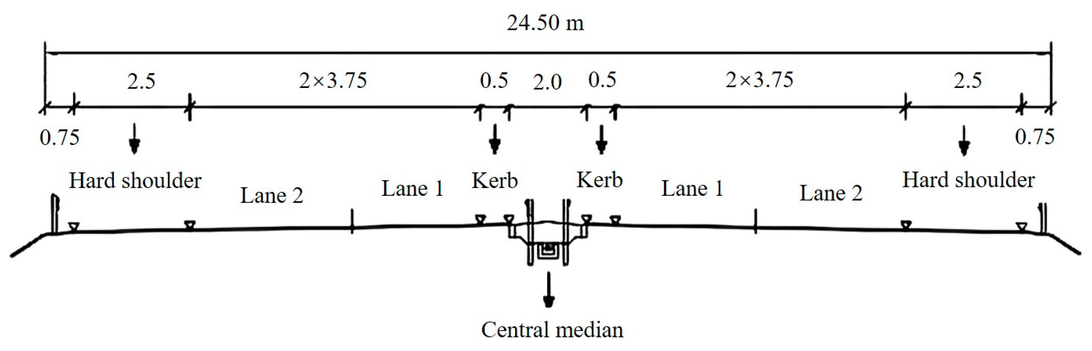
3.1. Geometric Data
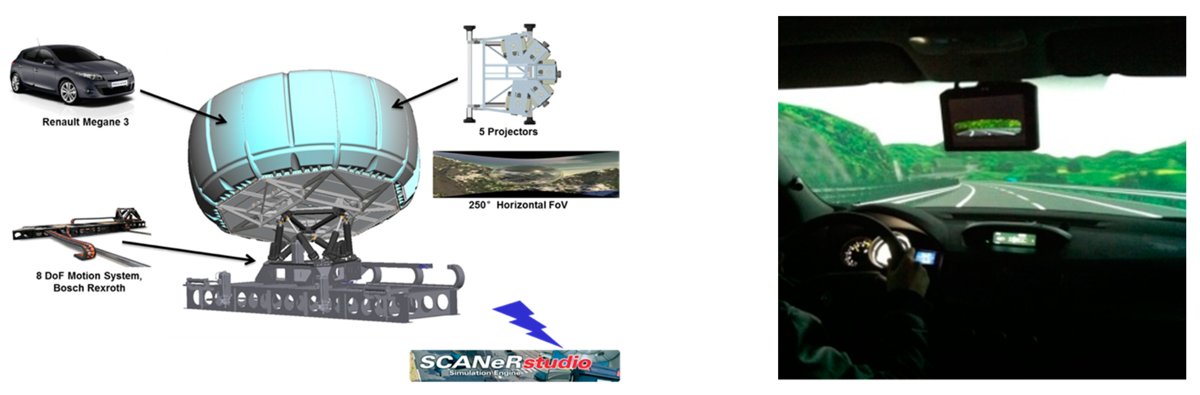
3.2. Micro-Driving Behavior Data Collection
4. Micro-Driving Behavior
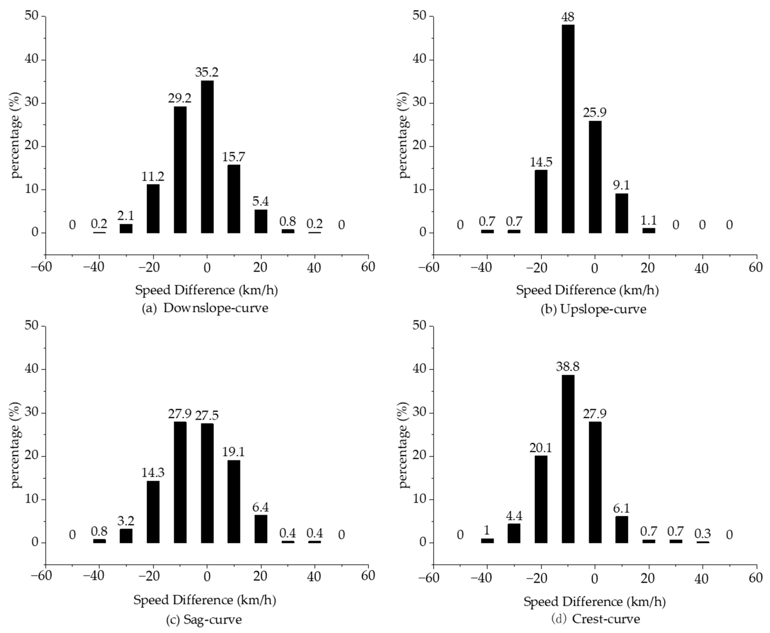
4.1. Speed Change Behavior
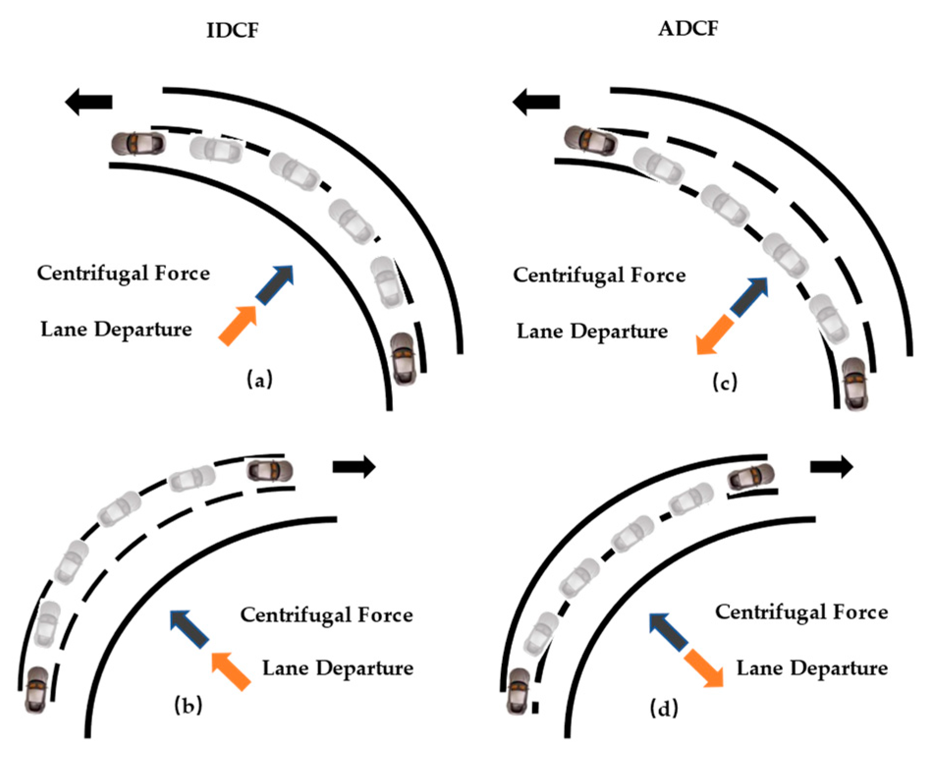
4.2. Lane Departure Behavior
4.3. Micro-Behavior Comparison of Four Combined Curves
5. Shapley Explanation for the Relationship between Micro-Behavior and Geometric Design
5.1. Methodology
5.1.1. Random Forest
5.1.2. SHAP
5.2. RF-SHAP Analysis of Mirco-Behavior on Combined Curves
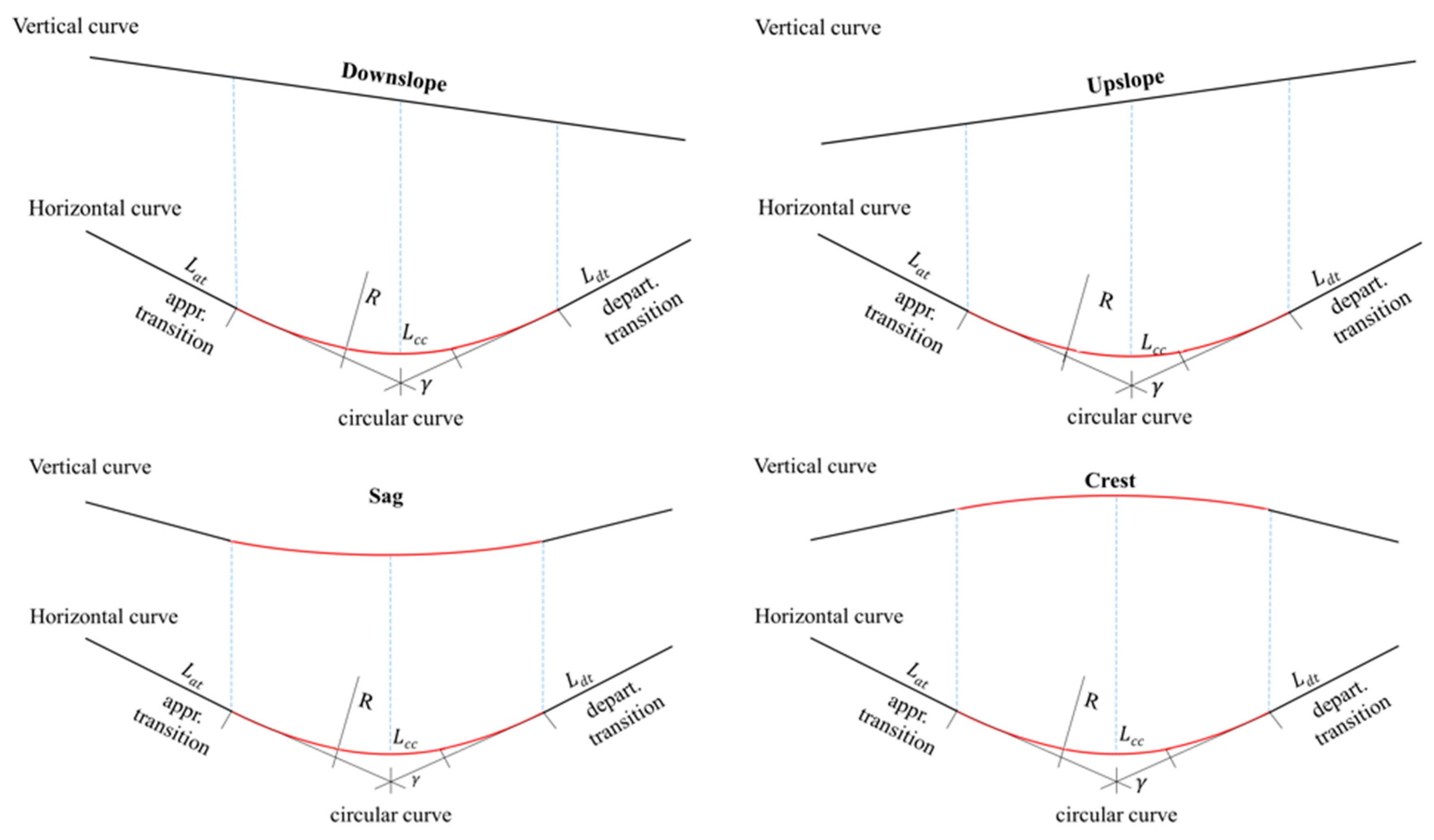
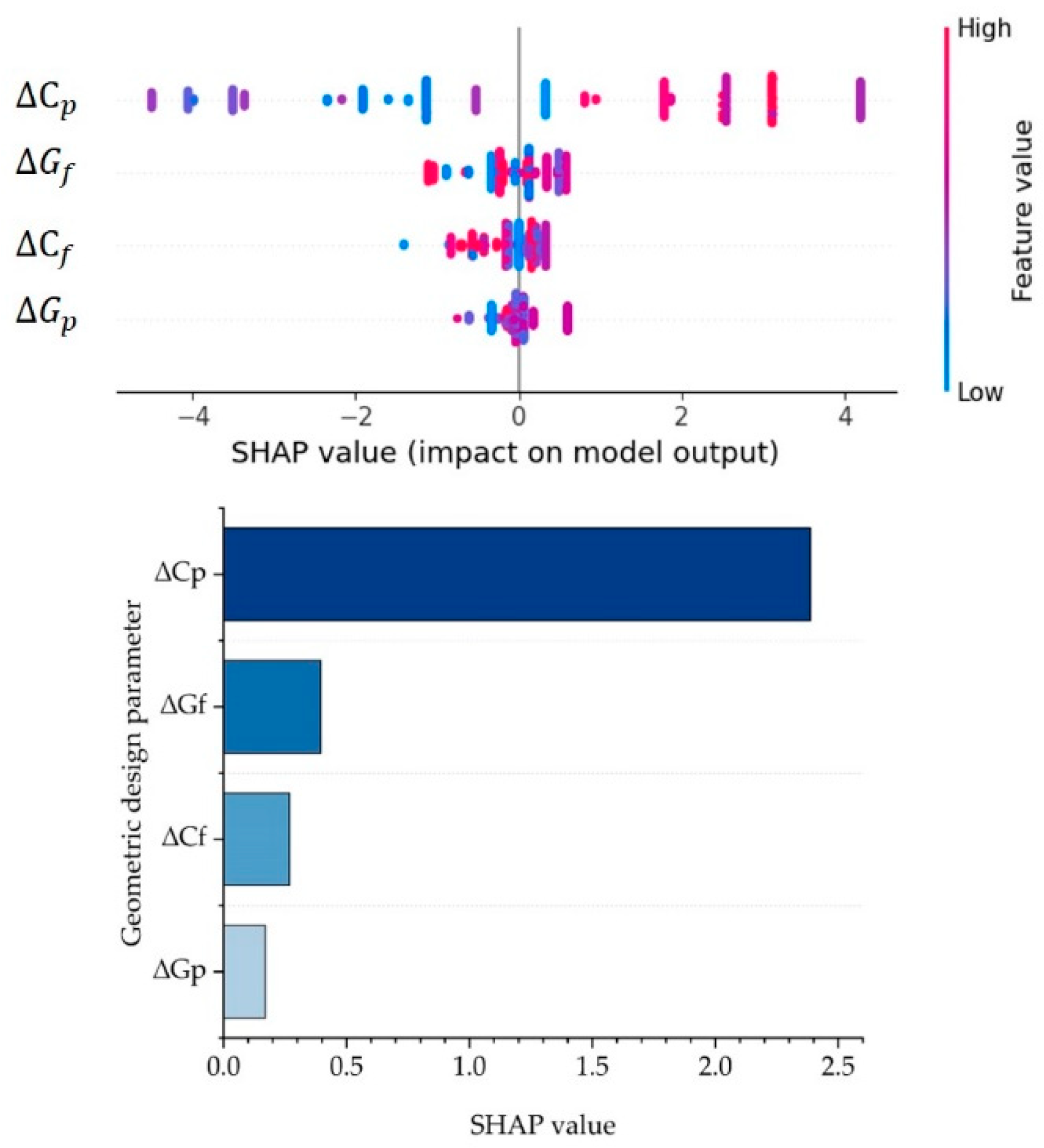
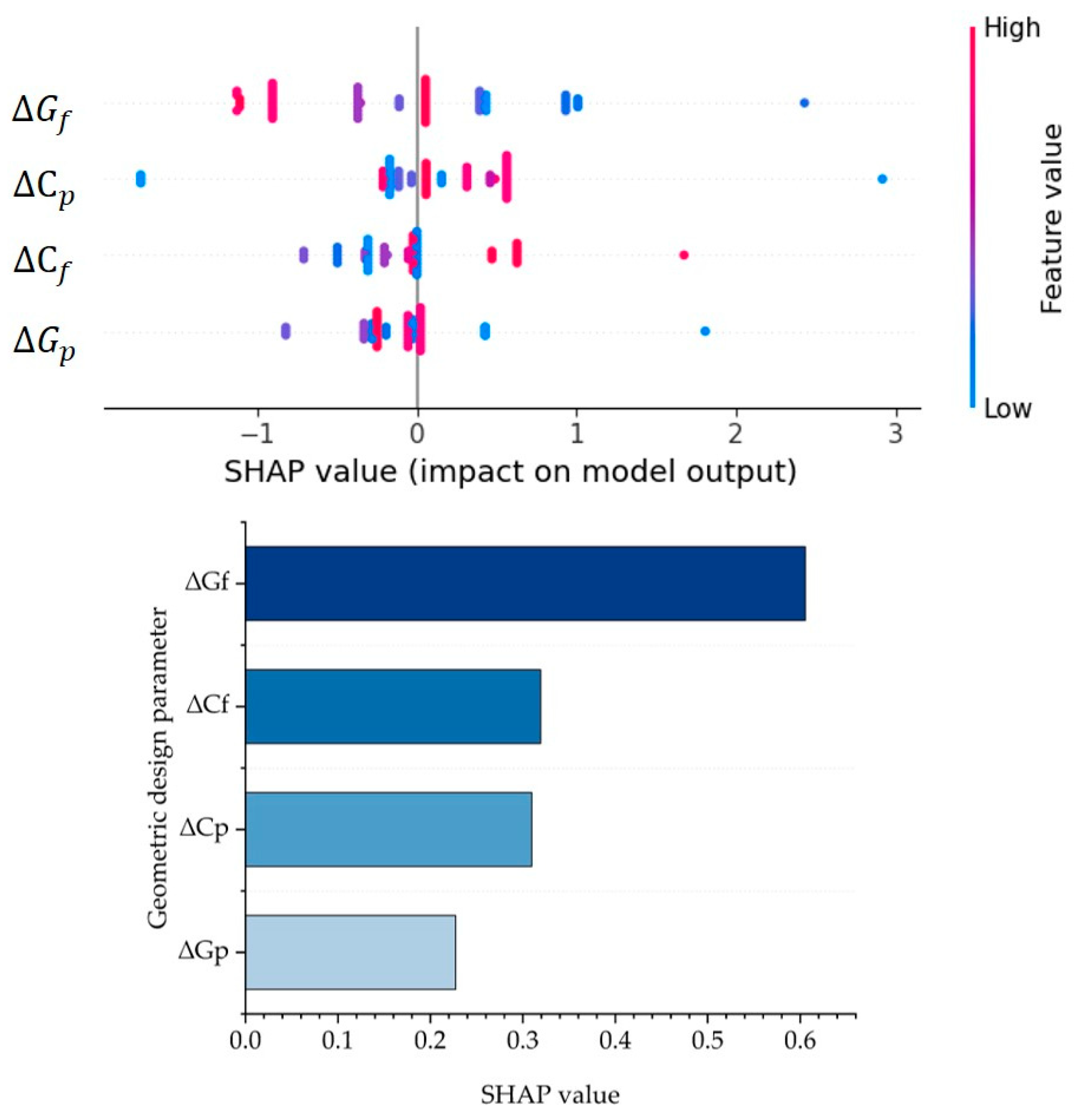
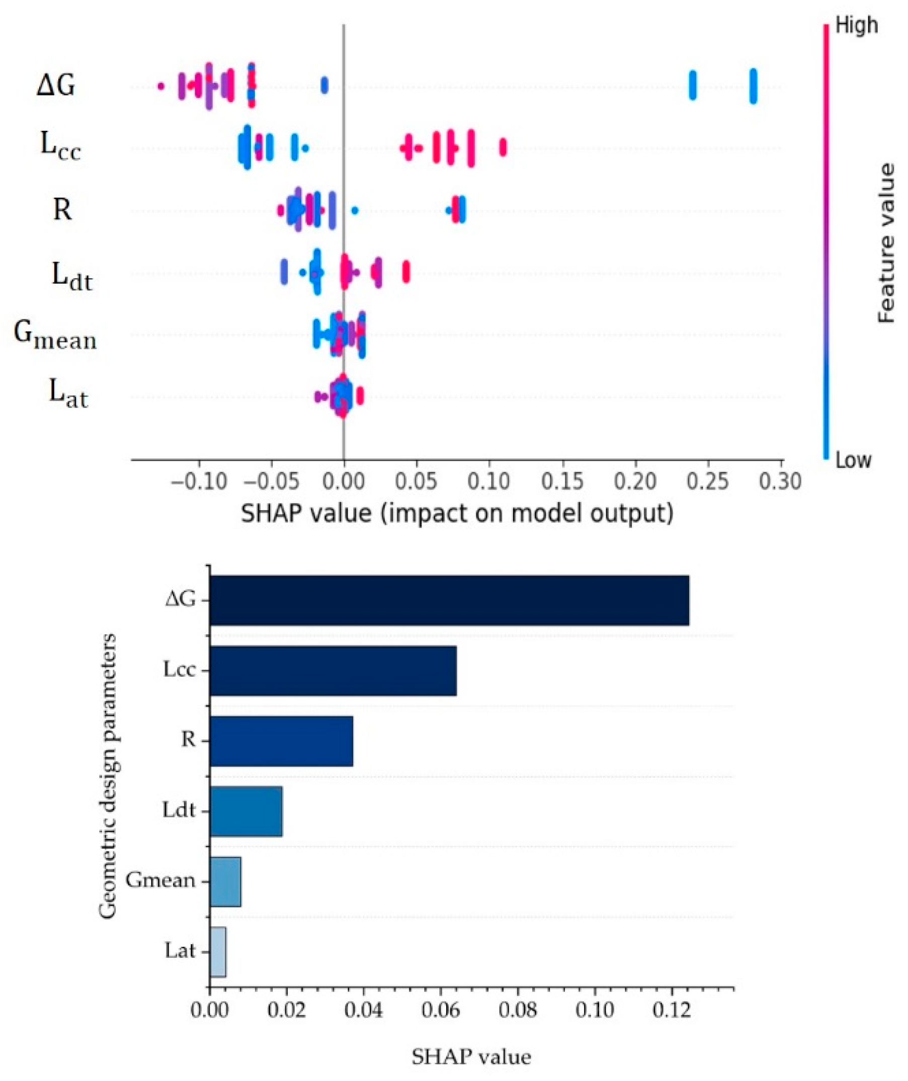
5.2.1. Speed Change Behavior on Downslope and Sag Curve
- (1)
- Downslope Curve
- (2)
- Sag Curve
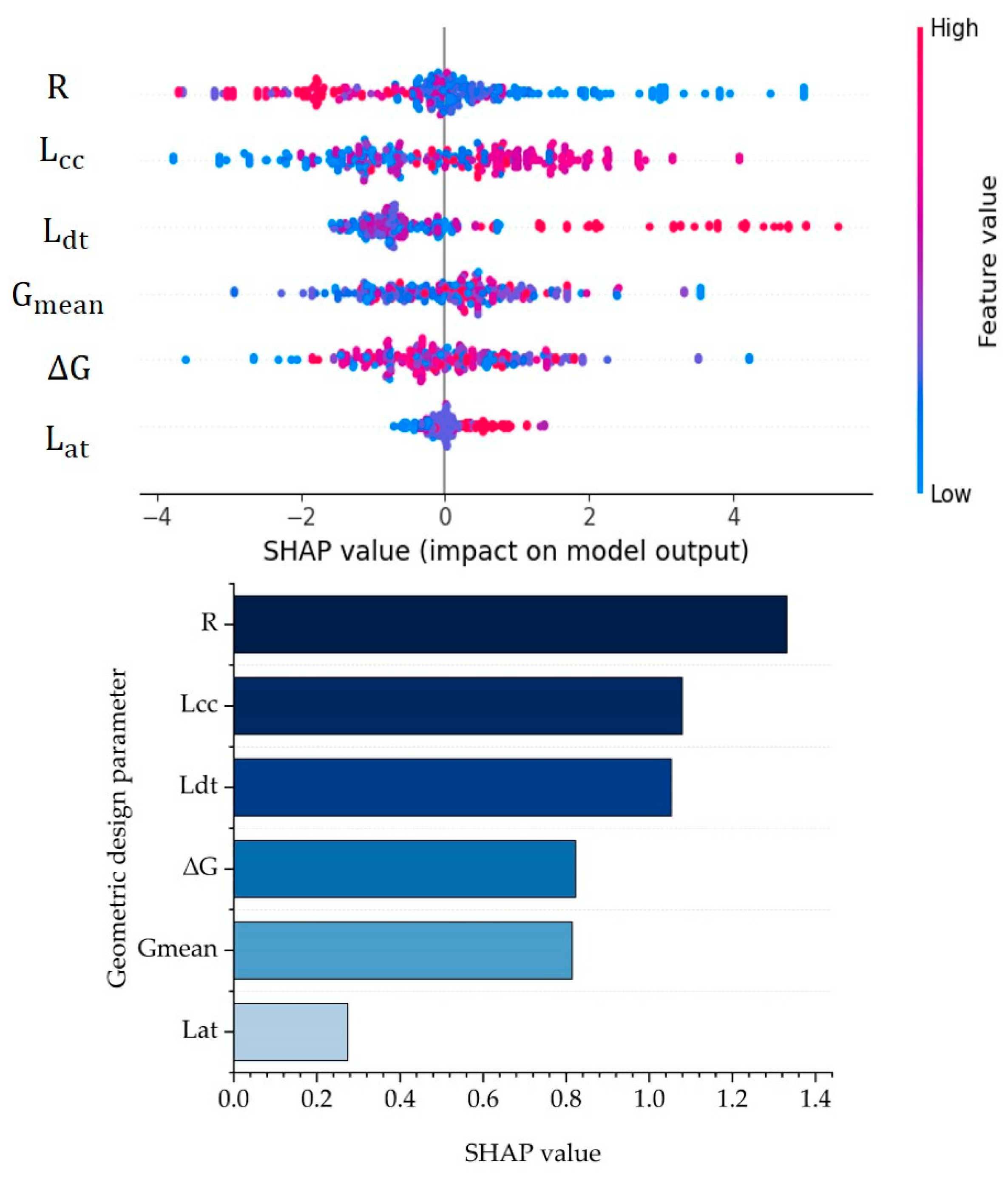
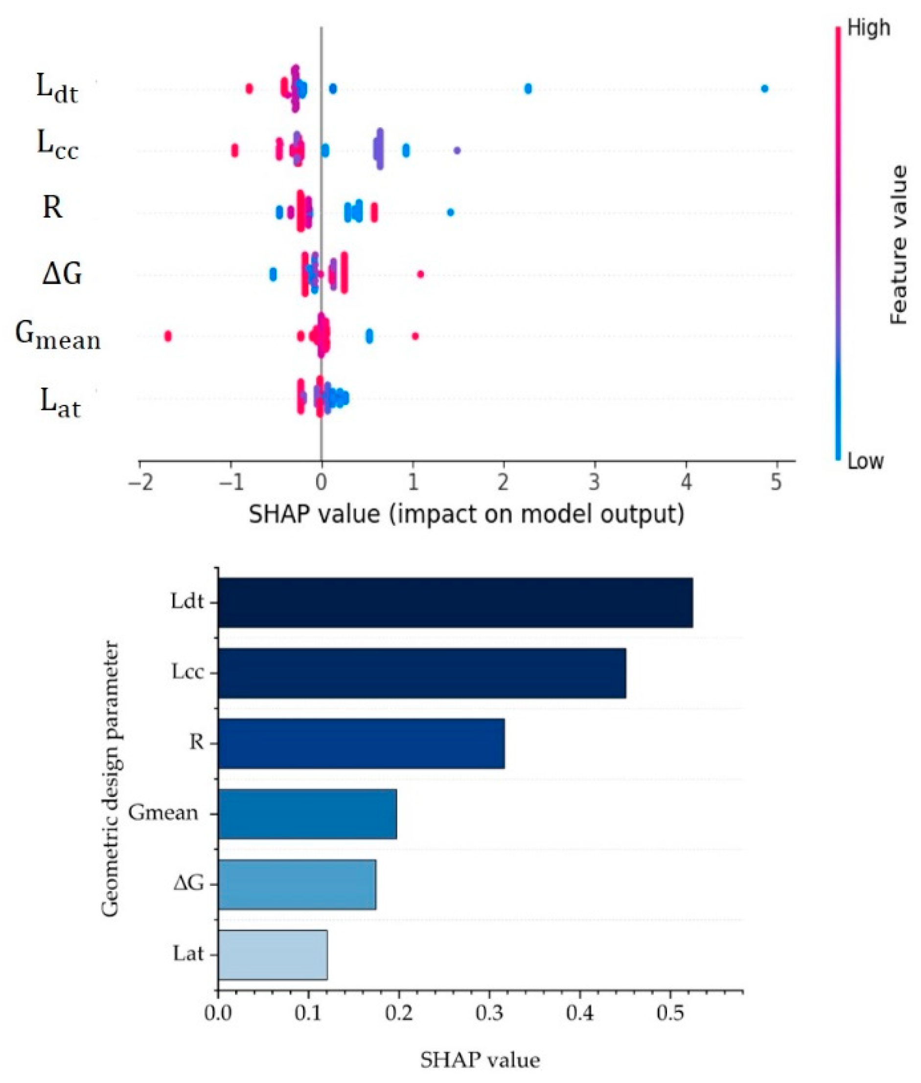
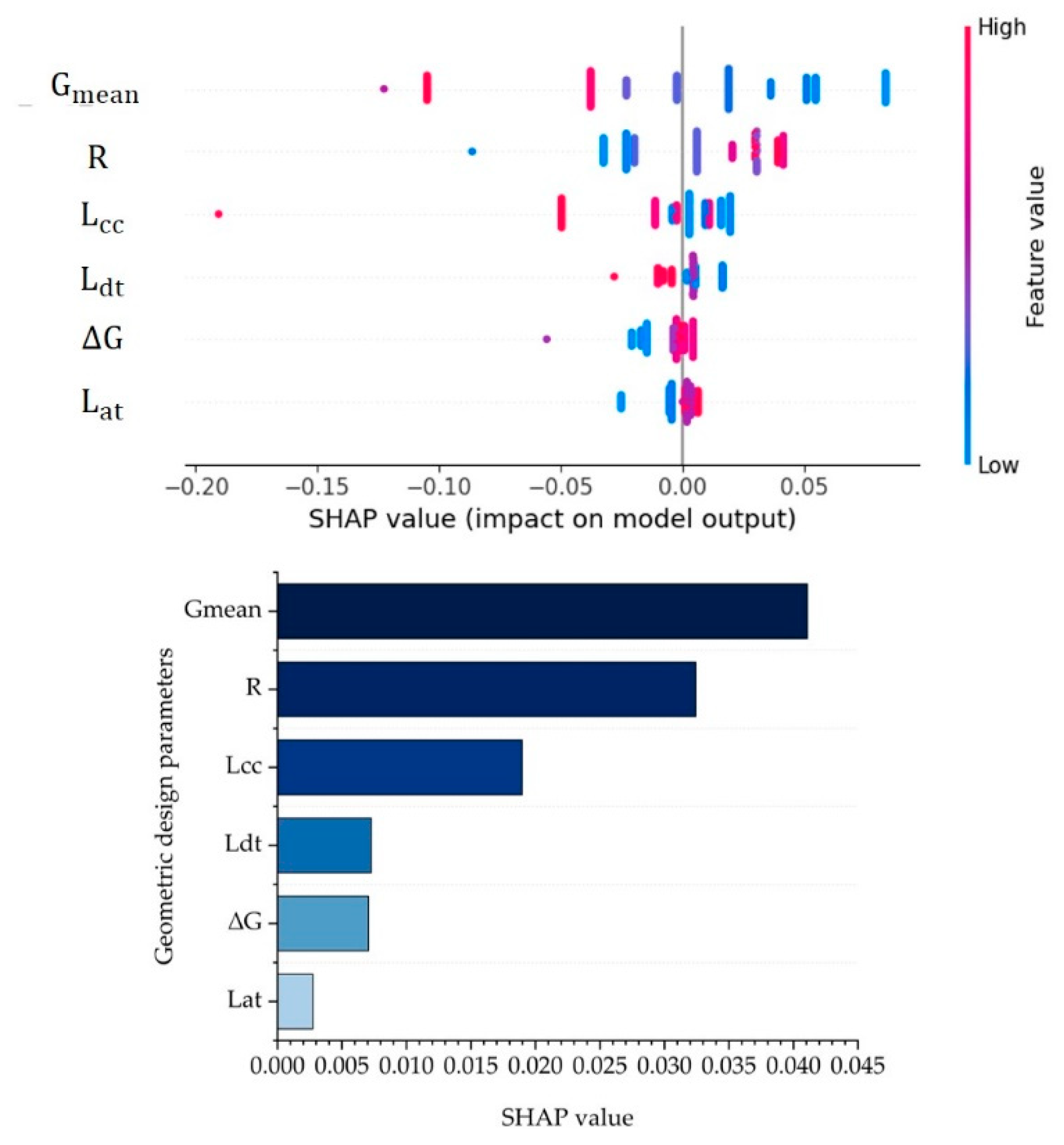
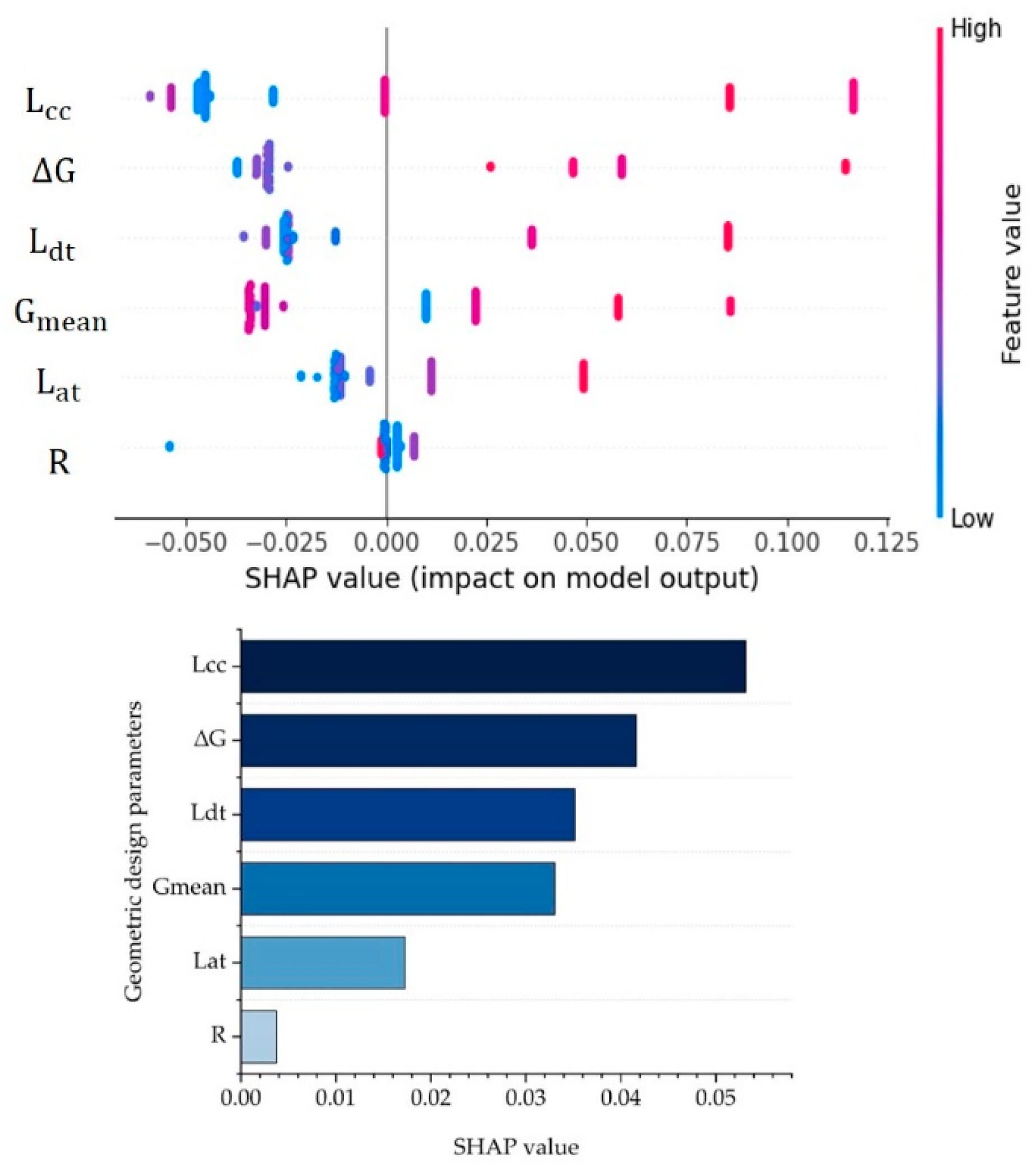
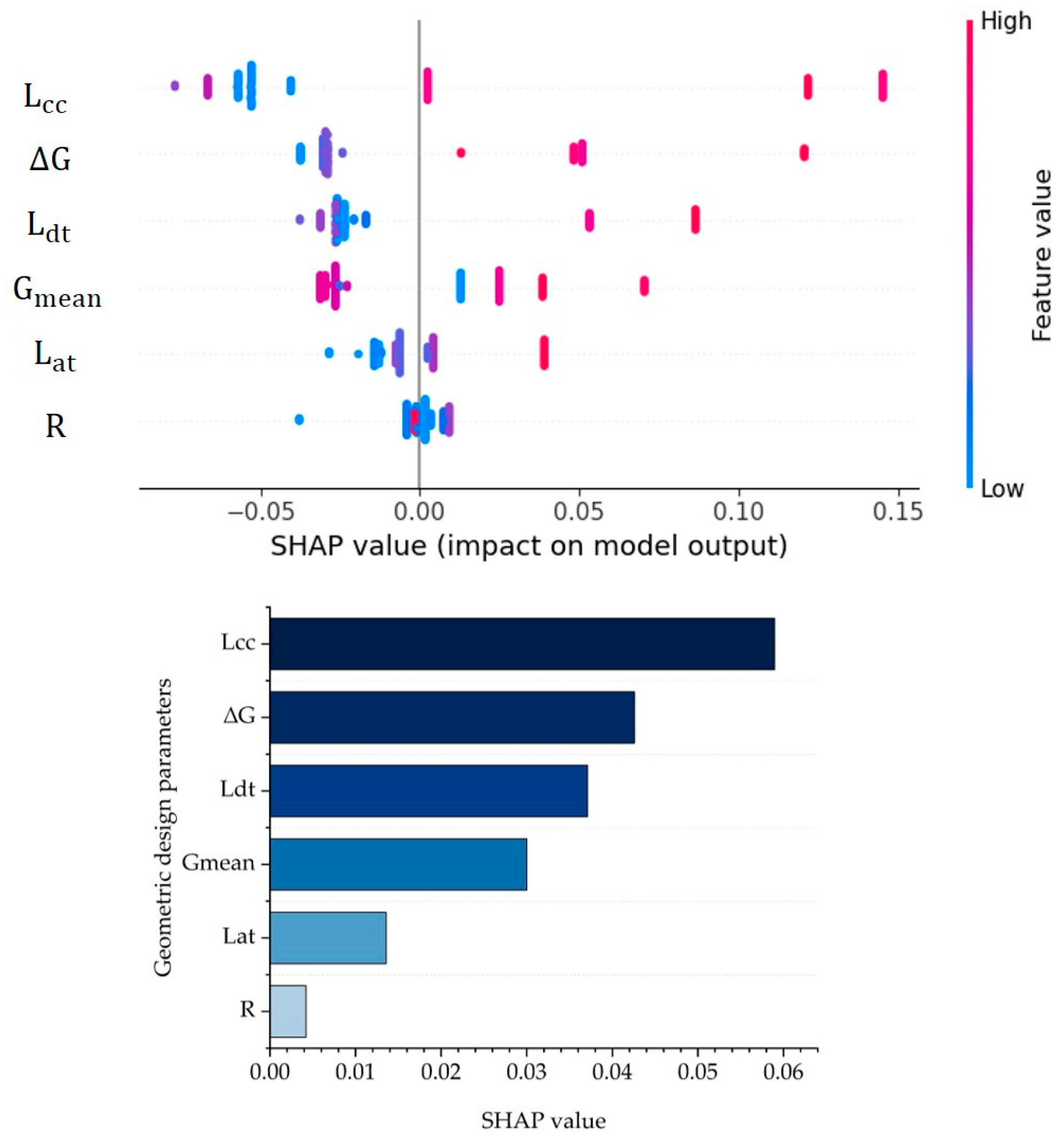
5.2.2. Lane Departure Behavior on Downslope, Upslope, and Crest Curves
- (1)
- Downslope Curve
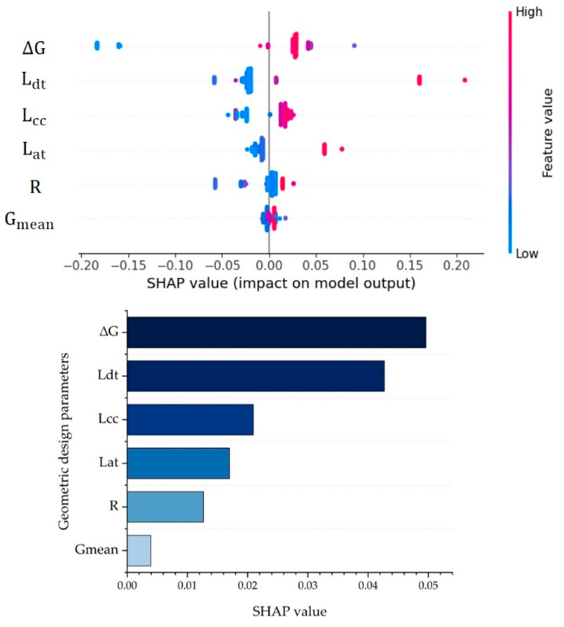
- (2)
- Upslope Curve
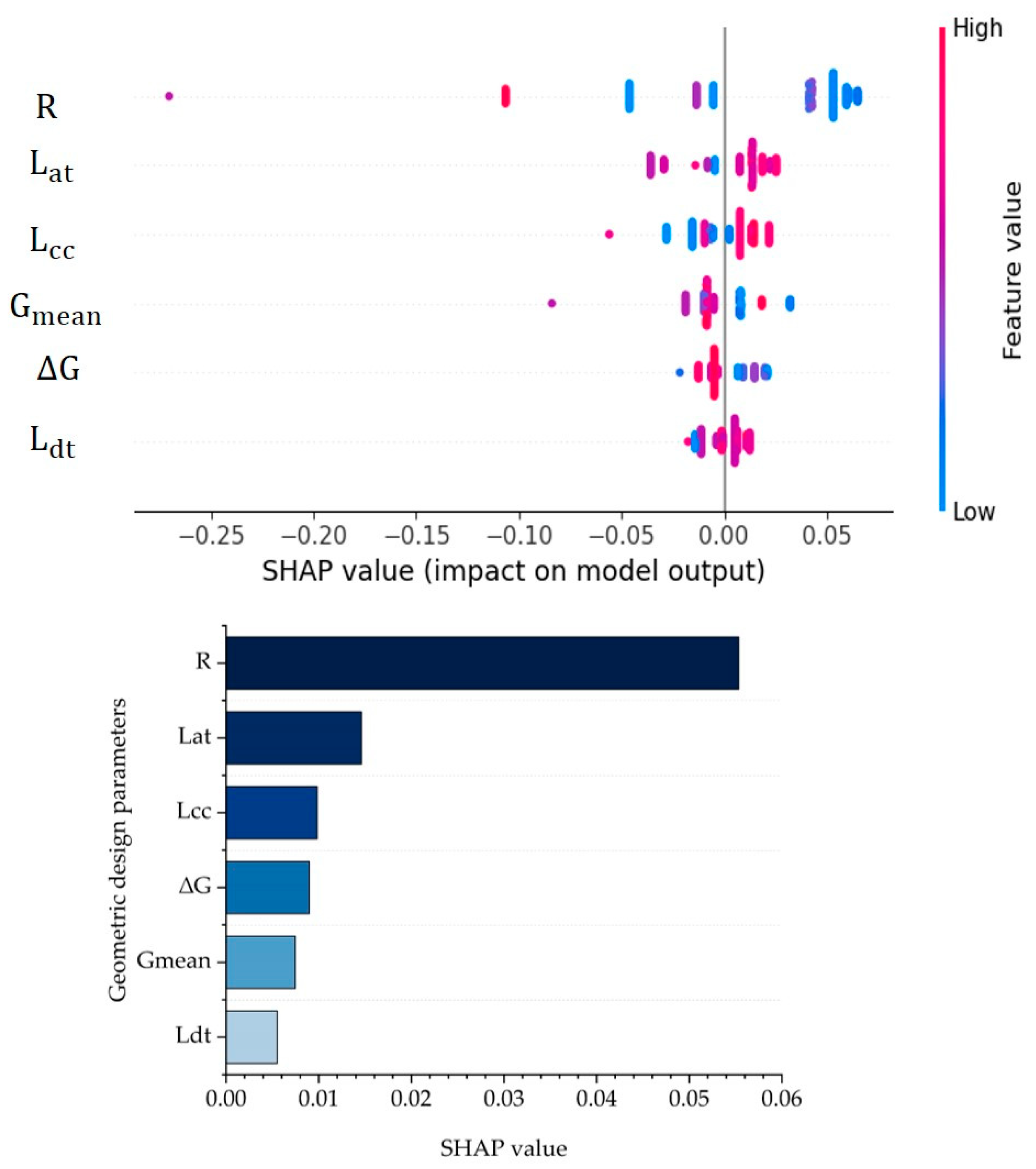
- (3)
- Crest Curve
6. Discussion
- Selecting key safety evaluation measures.
- Ranking of geometric design parameters of combined curves.
- Optimizing design based on safety evaluation measures.
7. Conclusions
Author Contributions
Funding
Institutional Review Board Statement
Informed Consent Statement
Data Availability Statement
Acknowledgments
Conflicts of Interest
References
- Chen, Z.; Wang, X.; Guo, Q. Effect of Combined Horizontal and Vertical Curve on Vehicle Longitudinal Acceleration of Mountainous Freeway. In Proceedings of the 19th COTA International Conference of Transportation Professionals, Nanjing, China, 6–8 July 2019. [Google Scholar]
- Chen, Z.; Wang, X.; Guo, Q.; Tarko, A. Towards Human-like Speed Control in Autonomous Vehicles: A Mountainous Freeway Case. Accid. Anal. Prev. 2022, 166, 106566. [Google Scholar] [CrossRef] [PubMed]
- American Association of State Highway and Transportation Officials (AASHTO). A Policy on Geometric Design of Highways and Streets; American Association of State Highway and Transportation Officials (AASHTO): Washington, DC, USA, 2018. [Google Scholar]
- Hanno, D. Effect of the Combination of Horizontal and Vertical Alignments on Road Safety. Master’s Thesis, The University of British Columbia, Vancouver, BC, Canada, 2004. [Google Scholar]
- Misaghi, P.; Hassan, Y. Modeling operating speed and speed differential on two-lane rural roads. J. Transp. Eng. 2005, 131, 408–418. [Google Scholar] [CrossRef]
- Nie, B.; Hassan, Y. Modeling driver speed behavior on horizontal curves of different road classifications. In Proceedings of the 84th Transportation Research Board Annual Meeting, Washington, DC, USA, 21–25 January 2007. [Google Scholar]
- Bella, F. Driving simulator for speed research on two-lane rural roads. Accid. Anal. Prev. 2008, 40, 1078–1087. [Google Scholar] [CrossRef] [PubMed]
- Sawtelle, A.; Shirazi, M.; Garder, P.E.; Rubin, J. Exploring the impact of seasonal weather factors on frequency of lane-departure crashes in Maine. J. Transp. Saf. Secur. 2022, 15, 445–466. [Google Scholar] [CrossRef]
- Destination Zero Deaths: Louisiana Strategic Highway Safety Plan. 2018. Available online: https://destinationzerodeaths.com/Images/Site%20Images/ActionPlans/SHSP.pdf (accessed on 7 November 2023).
- Zhou, X. Approach and Application of Steering on Freeway Curve Based on Visual Information; Wuhan University of Technology: Wuhan, China, 2010. [Google Scholar]
- Kazemzadehazad, S.; Monajjem, S.; Larue, G.S.; King, M.J. Evaluating new treatments for improving driver performance on combined horizontal and crest vertical curves on two-lane rural roads: A driving simulator study. Transp. Res. Part F Traffic Psychol. Behav. 2019, 62, 727–739. [Google Scholar] [CrossRef]
- Wang, X.; Wang, X. Speed Change Behavior on Combined Horizontal and Vertical Curves: Driving Simulator-based Analysis. Accid. Anal. Prev. 2018, 119, 215–224. [Google Scholar] [CrossRef]
- Haghighi, N.; Liu, X.C.; Zhang, G.; Porter, R.J. Impact of roadway geometric features on crash severity on rural two-lane highways. Accid. Anal. Prev. 2018, 11, 34–42. [Google Scholar] [CrossRef]
- Joseph, N.M.; Harikrishna, M.; Anjaneyulu, M.V.L.R. Safety Evaluation of Multiple Horizontal Curves Using Statistical Models. Int. J. Veh. Saf. 2021, 12, 81–97. [Google Scholar] [CrossRef]
- Fu, X.; He, S.; Du, J.; Ge, T. Effects of Spatial Geometric Mutation of Highway Alignments on Lane Departure at Curved Sections. Zhongguo Gonglu Xuebao/China J. Highw. Transp. 2019, 32, 106–114. [Google Scholar]
- Bella, F. Effects of Combined Curves on Driver’s Speed Behavior: Driving Simulator 40 Study. Transp. Res. Procedia 2014, 3, 100–108. [Google Scholar] [CrossRef]
- Wang, X.; Wang, T.; Tarko, A.; Tremont, P.J. The influence of combined alignments on lateral acceleration on mountainous freeways: A driving simulator study. Accid. Anal. Prev. 2015, 76, 110–117. [Google Scholar] [CrossRef] [PubMed]
- Peng, Y.; Geedipally, S.R.; Lord, D. Effect of Roadside Features on Single-Vehicle Roadway Departure Crashes on Rural Two-Lane Roads. Transp. Res. Rec. 2012, 2309, 21–29. [Google Scholar] [CrossRef]
- Roque, C.; Jalayer, M. Improving roadside design policies for safety enhancement using hazard-based duration modeling. Accid. Anal. Prev. 2018, 120, 165–173. [Google Scholar] [CrossRef] [PubMed]
- Wu, X.; Wang, X.; Lin, H.; He, Y.; Yang, L. Evaluating Alignment Consistency for Mountainous Freeway in Design Stage: Driving Simulator-Based Approach. In Proceedings of the 92th Annual Meeting of the Transportation Research Board, Washington, DC, USA, 13–17 January 2013. [Google Scholar]
- Kennedy, R.S.; Lane, N.E.; Berbaum, K.S.; Lilienthal, M.G. Simulator sickness questionnaire: An enhanced method for quantifying simulator sickness. Int. J. Aviat. Psychol. 1993, 3, 203–220. [Google Scholar] [CrossRef]
- Hunan Bureau of Statistics. Available online: https://tjj.hunan.gov.cn/hntj/tjfx/jmxx/2014jmxx/201507/t20150717_3785983.html (accessed on 24 January 2024).
- The Central People’s Government of the People’s Republic of China. Available online: https://www.gov.cn/gongbao/content/2022/content_5679696.htm?eqid=b59297960001ed3600000003645a02a2 (accessed on 24 January 2024).
- Wang, X.; Wang, X.; Cai, B.; Liu, J. Combined alignment effects on deceleration and acceleration: A driving simulator study. Transp. Res. Part C Emerg. Technol. 2019, 104, 172–183. [Google Scholar] [CrossRef]
- Dogru, N.; Subasi, A. Traffic accident detection using random forest classifier. In Proceedings of the 2018 15th Learning and Technology Conference (L & T), Jeddah, Saudi Arabia, 25–26 February 2018. [Google Scholar]
- Han, T.; Jiang, D.; Zhao, Q.; Wang, L.; Yin, K. Comparison of random forest, artificial neural networks and support vector machine for intelligent diagnosis of rotating machinery. Trans. Inst. Meas. Control 2017, 40, 2681–2693. [Google Scholar] [CrossRef]
- Zhu, C.; Brown, C.T.; Dadashova, B.; Ye, X.; Sohrabi, S.; Potts, I. Investigation on the driver-victim pairs in pedestrian and bicyclist crashes by latent class clustering and random forest algorithm. Accid. Anal. Prev. 2023, 182, 106964. [Google Scholar] [CrossRef]
- Gu, Y.; Liu, D.; Arvin, R.; Khattak, A.J.; Han, L.D. Predicting intersection crash frequency using connected vehicle data: A framework for geographical random forest. Accid. Anal. Prev. 2023, 179, 106880. [Google Scholar] [CrossRef]
- Kang, K.; Ryu, H. Predicting types of occupational accidents at construction sites in Korea using random forest model. Saf. Sci. 2019, 120, 226–236. [Google Scholar] [CrossRef]
- Choi, J.; Gu, B.; Chin, S.; Lee, J.-S. Machine learning predictive model based on national data for fatal accidents of construction workers. Autom. Constr. 2020, 110, 102974. [Google Scholar] [CrossRef]
- Gatera, A.; Kuradusenge, M.; Bajpai, G.; Mikeka, C.; Shrivastava, S. Comparison of random forest and support vector machine regression models for forecasting road accidents. Sci. Afr. 2023, 21, e01739. [Google Scholar] [CrossRef]
- Su, Z.; Liu, Q.; Zhao, C.; Sun, F.A. Traffic Event Detection Method Based on Random Forest and Permutation Importance. Mathematics 2022, 10, 873. [Google Scholar] [CrossRef]
- Yan, M.; Shen, Y. Traffic Accident Severity Prediction Based on Random Forest. Sustainability 2022, 14, 1729. [Google Scholar] [CrossRef]
- Lundberg, S.M.; Lee, S.I. A unified approach to interpreting model predictions. In Proceedings of the Advances in Neural Information Processing Systems 30: Annual Conference on Neural Information Processing Systems 2017, Long Beach, CA, USA, 4–9 December 2017. [Google Scholar]
- Wen, X.; Xie, Y.; Jiang, L.S.; Pu, Z.; Ge, T. Applications of machine learning methods in traffic crash severity modelling: Current status and future directions. Transp. Rev. 2021, 41, 855–879. [Google Scholar] [CrossRef]
- Tamim Kashifi, M.; Jamal, A.; Samim Kashefi, M.; Almoshaogeh, M.; Masiur Rahman, S. Predicting the travel mode choice with interpretable machine learning techniques: A comparative study. Travel Behav. Soc. 2022, 29, 279–296. [Google Scholar] [CrossRef]
- Sarwar, M.T.; Anastasopoulos, P.C.; Golshani, N.; Hulme, K.F. Grouped random parameters bivariate probit analysis of perceived and observed aggressive driving behavior: A driving simulation study. Anal. Methods Accid. Res. 2017, 13, 52–64. [Google Scholar] [CrossRef]
- Wang, X.; Li, S.; Li, X.; Wang, Y.; Zeng, Q. Effects of geometric attributes of horizontal and sag vertical curve combinations on freeway crash frequency. Accid. Anal. Prev. 2023, 186, 107056. [Google Scholar] [CrossRef] [PubMed]
- Li, X.; Guo, Z.; Li, Y. Driver operational level identification of driving risk and graded time-based alarm under near-crash conditions: A driving simulator study. Accid. Anal. Prev. 2022, 166, 106544. [Google Scholar] [CrossRef]
- Ma, Y.; Wang, F.; Chen, S.; Xing, G.; Xie, Z.; Wang, F. A dynamic method to predict driving risk on sharp curves using multi-source data. Accid. Anal. Prev. 2023, 191, 107228. [Google Scholar] [CrossRef]
- Ministry of Transport of the People’s Republic of China. Design Specification for Highway Alignment; China Communications Press: Beijing, China, 2017.


| Continuous Variable | |||||
|---|---|---|---|---|---|
| Variables | Description | Mean | S.D. | Min | Max |
| Mean slope of combined curve | −2.23 | 2.39 | −5.25 | 5.25 | |
| Slope differential of maximum and minimum slope | 2.86 | 1.93 | 0.00 | 8.10 | |
| Length of combined curve | 413.97 | 135.35 | 222.51 | 790.76 | |
| Length of circular curve | 211.13 | 122.64 | 35.00 | 490.76 | |
| Length of approach transition | 101.10 | 25.30 | 0.00 | 160.00 | |
| Length of departure transition | 101.74 | 25.08 | 0.00 | 155.00 | |
| Radius of combined curve | 821.56 | 447.23 | 400.00 | 2500.00 | |
| Variables | Description | Mean | S.D. | Min | Max |
|---|---|---|---|---|---|
| 1 | The preceding curvature change | 0.00079 | 0.00048 | 0.00004 | 0.0020 |
| 2 | The slope change of the preceding section | 3.45 | 3.57 | 0.00 | 12.00 |
| 3 | The following curvature change | 0.00079 | 0.0005 | 0.00005 | 0.0024 |
| 4 | The slope change of the following section | 1.93226 | 1.93277 | 0.00 | 9.00 |
| Curve | Minimum Value | Maximum Value | S.D. | 7.5th Percentile Value | 92.5th Percentile Value |
|---|---|---|---|---|---|
| Downslope | −39.96 | 42.30 | 11.98 | −15.17 | 17.94 |
| Upslope | −41.88 | 29.57 | 9.71 | −14.49 | 12.80 |
| Sag | −32.32 | 40.24 | 13.53 | −17.83 | 19.91 |
| Crest | −35.03 | 42.53 | 11.12 | −17.48 | 12.59 |
| Type | Mean (m) | Max (m) | Min (m) | S.D (m) | |
|---|---|---|---|---|---|
| IDCF lane departure | Maximum lateral departure | 0.81 | 1.10 | 0.01 | 0.29 |
| Departure persistence distance | 72.75 | 500 | 5 | 70.48 | |
| ADCF lane departure | Maximum lateral departure | 0.36 | 1.52 | 0.00 | 0.35 |
| Departure persistence distance | 60.64 | 410 | 5 | 61.93 | |
| Road Type | Speed Change | Lane Departure |
|---|---|---|
| Upslope curve | 4.436 | 19.753 |
| Downslope curve | 15.884 | 41.114 |
| Crest curve | 8.435 | 12.482 |
| Sag curve | 5.111 | 2.203 |
Disclaimer/Publisher’s Note: The statements, opinions and data contained in all publications are solely those of the individual author(s) and contributor(s) and not of MDPI and/or the editor(s). MDPI and/or the editor(s) disclaim responsibility for any injury to people or property resulting from any ideas, methods, instructions or products referred to in the content. |
© 2024 by the authors. Licensee MDPI, Basel, Switzerland. This article is an open access article distributed under the terms and conditions of the Creative Commons Attribution (CC BY) license (https://creativecommons.org/licenses/by/4.0/).
Share and Cite
Wang, X.; Wei, X.; Wang, X. Investigating Micro-Driving Behavior of Combined Horizontal and Vertical Curves Using an RF Model and SHAP Analysis. Appl. Sci. 2024, 14, 2369. https://doi.org/10.3390/app14062369
Wang X, Wei X, Wang X. Investigating Micro-Driving Behavior of Combined Horizontal and Vertical Curves Using an RF Model and SHAP Analysis. Applied Sciences. 2024; 14(6):2369. https://doi.org/10.3390/app14062369
Chicago/Turabian StyleWang, Xiaomeng, Xuanzong Wei, and Xuesong Wang. 2024. "Investigating Micro-Driving Behavior of Combined Horizontal and Vertical Curves Using an RF Model and SHAP Analysis" Applied Sciences 14, no. 6: 2369. https://doi.org/10.3390/app14062369
APA StyleWang, X., Wei, X., & Wang, X. (2024). Investigating Micro-Driving Behavior of Combined Horizontal and Vertical Curves Using an RF Model and SHAP Analysis. Applied Sciences, 14(6), 2369. https://doi.org/10.3390/app14062369