Influence of Frictional Stress Models on Simulation Results of High-Pressure Dense-Phase Pneumatic Conveying in Horizontal Pipe

Abstract

Based on the two-fluid model, a three-zone drag model was developed, and the kinetic theory of granular flows and the Schneiderbauer solids wall boundary model were modified to establish a new three-dimensional (3D) unsteady mathematical model for high-pressure dense-phase pneumatic conveying in horizontal pipe. With this mathematical model, the influence of the three frictional stress models, namely Dartevelle frictional stress model, Srivastava and Sundaresan frictional stress model, and the modified Berzi frictional stress model, on the simulation result was explored. The simulation results showed that the three frictional stress models accurately predicted the pressure drop and its variations with supplementary gas in the horizontal pipe, with relative errors ranging from −4.91% to +7.60%. Moreover, the predicted solids volume fraction distribution in the cross-section of the horizontal pipe using these frictional stress models exhibited good agreement with the electrical capacitance tomography (ECT) images. Notably, the influence of the three frictional stress models on the simulation results was predominantly observed in the transition region and deposited region. In the deposited region, stronger frictional stress resulting in lower solids volume fraction and a higher pressure drop in the horizontal pipe were observed. Among the three frictional stress models, the simulation results with the modified Berzi frictional stress model aligned better with the experimental data. Therefore, the modified Berzi frictional stress model is deemed more suitable for simulating high-pressure dense-phase pneumatic conveying in horizontal pipe.

1. Introduction

To facilitate the achievement of China’s dual carbon goals (DCGs), it is imperative to actively develop the clean utilization technology of coal resources, specifically through clean coal technology. Among various clean coal technologies, coal gasification stands out as one of the most notable approaches. In particular, large-scale high-efficiency entrained-flow coal gasification technology has emerged as the most promising coal gasification method [1], and high-pressure dense-phase pneumatic conveying is a crucial component of this gasification technology.

High-pressure dense-phase pneumatic conveying is widely applied in energy, chemical, metallurgical, power generation, pharmaceutical, and food processing industries due to its advantages, such as low gas velocity, high solid–gas ratio, low energy consumption, reduced gas consumption, and minimal pipeline wear. In the solid processing industry, it is estimated that the market value of the conveying systems could increase to £30 billion by 2025 [2]. Therefore, high-pressure dense-phase pneumatic conveying technology possesses significant market competitiveness and development potential. However, due to its high pressure, high solids volume fraction, and complex flow characteristics [3,4], as well as numerous influencing factors (such as carrier gas properties, material properties, operating parameters, conveying parameters, and pipeline shape), the conveying characteristics of high-pressure dense-phase pneumatic conveying are extremely complex. Currently, the understanding of the conveying mechanism and characteristics remains inadequate. Many issues have not been properly addressed for high-pressure dense-phase pneumatic conveying, thus hindering its comprehensive and rational utilization in engineering applications.

Horizontal pipes are crucial and commonly used pipelines in high-pressure dense-phase pneumatic conveying, generally accounting for the highest proportion of the whole conveying pipeline. However, during the conveying process in horizontal pipe, various types of metastable flow patterns, such as dune flow and slug flow, are prone to occur. And these flow patterns directly affect the stability of the conveying process and may even result in pipe blockages and conveying interruptions. In a sense, the stable and reliable operation of high-pressure dense-phase pneumatic conveying in horizontal pipe is the basic prerequisite and fundamental guarantee for the stable production of large-scale, high-efficiency, entrained-flow coal gasification systems. Therefore, the study of high-pressure dense-phase pneumatic conveying in horizontal pipe is of great practical significance.

There are two main research methods for high-pressure dense-phase pneumatic conveying: experimental research and simulation research. Current research mainly focuses on the experimental research field of high-pressure dense-phase pneumatic conveying. Numerous scholars have conducted a large number of experimental studies from various perspectives using existing measurement techniques and equipment, yielding several valuable results related to pipeline resistance characteristics, flow patterns, conveying characteristics and stability [5,6,7,8,9,10]. As is known, pneumatic conveying is a highly comprehensive discipline that involves multiple fields, such as fluid mechanics, mechanical engineering, and particle science. In particular, high-pressure dense-phase pneumatic conveying exhibits intricate nonlinear and non-equilibrium dynamic characteristics. However, the existing experimental equipment and measurement techniques are severely limited, making many crucial parameters for high-pressure dense-phase pneumatic conveying challenging to measure. As a result, the current state of experimental research has reached a bottleneck stage [6].

With the rapid development of computational fluid dynamics theory and the fast improvement of computer performance, simulation methods have become powerful research tools widely applied in the field of pneumatic conveying. In particular, computational fluid dynamics (CFD) has played an important role in analyzing high-pressure dense-phase pneumatic conveying. Compared to experimental research methods, simulation methods can capture real-time comprehensive flow field information of each cell in the computational domain, including detailed micro-characteristic parameters [11], which facilitates thorough analysis and understanding of the conveying characteristics and flow mechanism. Additionally, simulation methods are more efficient, convenient, and cost-effective, serving as an important supplement to experimental research methods, and provide a reliable theoretical foundation and practical guidance for the rational design and comprehensive optimization of high-pressure dense-phase pneumatic conveying.

The simulation approaches can be broadly categorized into the Euler-Lagrangian approach and the Euler-Euler approach. The Euler-Lagrangian approach provides microscopic details, such as on particle trajectories and forces acting on individual particle, which are essential for understanding gas–solid systems [12,13,14]. Hence, this approach is considered to be more accurate and efficient for gas–solid systems involving particles of different sizes or densities [15]. Numerous simulation studies of pneumatic conveying have been conducted using the Euler-Lagrangian approach by both domestic and foreign researchers [16]. However, due to the requirement for small time steps to accurately simulate particle–particle/wall collisions with relatively high accuracy., the Euler-Lagrangian approach necessitates high computational resources, particularly for dense-phase pneumatic conveying. To reduce the computational cost of this approach, several new methods have been proposed, including the CFD-discrete element method (CFD–DEM), the coarse-grained discrete element method (CGDEM), and the multiphase particle-in-cell method (MP–PIC). These methods aim to develop scaling theories and accelerate simulations of gas-solid systems [11,17]. For instance, MP–PIC considers a specific group of particles with similar properties (e.g., species, size, density, temperature) as a parcel, to decrease the number of particles involved in the computations [18]. Nevertheless, these new methods have excessively high computational requirements for large-scale industrial applications, such as dense-phase pneumatic conveying systems with billions of particles. Furthermore, the scaling theories, derived from force balances between coarse-grained or parcel particles and their corresponding original particles, introduce uncertainties in the modeling process, particularly in determining parcel particle properties and precise particle–particle/wall interactions [12,19].

The continuum approach, represented by the two-fluid model (TFM), is more suitable for dense-phase pneumatic conveying due to its computational convenience and efficiency. As a result, an increasing number of researchers have used the Euler–Euler approach for simulating high-pressure dense-phase pneumatic conveying. Ratnayaka et al. [20] conducted simulation research on horizontal bends using two-fluid modelling, producing simulation results that indicated the two-fluid modelling has great potential in predicting the conveying characteristics of dense-phase pneumatic conveying. Inspired by Ratnayaka’s work, many scholars have gradually improved the constitutive relationships of dense-phase pneumatic conveying and conducted relevant simulation research from different perspectives. For instance, Zhong et al. [21] introduced the kinetic theory of granular flow to simulate the gas–solid two-phase flow in the spouted bed and restructured a three-dimensional steady-state mathematical model to investigate the effects of non-ideal particle collisions on the restitution coefficient. Subsequently, Ma et al. [22] further considered the unsteady-state conveying characteristics and established a three-dimensional unsteady-state mathematical model for dense-phase pneumatic conveying. They explored the impact of material properties, wall roughness, and bend curvature on the conveying characteristics in vertical bends. However, dense-phase pneumatic conveying is highly susceptible to particle deposition in horizontal pipes and bends. Hence, Wang et al. [23] introduced a frictional stress model to study the conveying characteristics of high-pressure dense-phase pneumatic conveying in horizontal pipe, producing simulation results that showed improved accuracy when frictional stress was considered. However, the underlying mechanisms of the frictional stress model were not revealed in this study.

In dense-phase pneumatic conveying, the solids volume fraction is extremely high, approaching the bulk packing volume fraction (about 0.5 for pulverized coal). During this process, particles are mainly in sustained contact, resulting in the solids stress primarily originating from frictional stress [24,25,26,27]. Consequently, the impact of frictional stress on high-pressure dense-phase pneumatic conveying is of utmost importance, although there is limited literature on this topic. Johnson and Jackson [28,29] were the pioneers in proposing the frictional pressure model, introducing three dimensionless coefficients (Fr, r, s) to characterize the frictional properties of different materials. Simultaneously, on the basis of the von Mises yield criterion, Schaeffer [30] proposed a solids frictional viscosity model. However, Nikolopoulos et al. [31,32] found that the von Mises/Coulomb yield criterion, originating from soil mechanics, cannot fully apply to the simulation for dense-phase gas-solid flow of pulverized coal since it can properly predict dilatancy but not consolidation for the solids phase. To overcome this limitation, Srivastava and Sundaresan [33] incorporated the strain rate term proposed by Savage [34] and soil mechanics theory [35,36] into modifying the Schaeffer frictional viscosity model on the basis of the extended von Mises yield criterion. They combined the Johnson and Jackson frictional pressure model to establish a comprehensive frictional stress model. Then this model was applied to simulate the gas–solid flow in the fluidized bed, validating its reliability. Dartevelle [25] set up a new frictional stress model by combining the Pitman–Schaeffer–Gray–Stiles yield criterion, which considers both the dilatancy and consolidation of the solids phase in dense-phase gas–solid flow. And the model was validated through simulations of soil particle flows in geophysics. Pu et al. [37] made modifications to the Johnson and Jackson frictional pressure model [28,29] and the Syamlal frictional viscosity model [38] to establish the frictional stress model. Coupling this frictional stress model with the classical particle kinetic theory, they conducted a three-dimensional simulation of high-pressure dense-phase pneumatic conveying in horizontal pipe. The study provided insights into the flow patterns and pressure drop of high-pressure dense-phase pneumatic conveying in horizontal pipe, and the simulation reliability was verified by comparisons with the experimental data. Wang Ying et al. [39] coupled the classical kinetic theory of granular flows (KTGF) with Schaeffer frictional stress model to simulate bypass dense-phase pneumatic conveying. The results showed substantial improvement in predicting pressure drop after considering the frictional stress model, although the experimental pressure drop remained underestimated. Therefore, they introduced an offset volume fraction to alleviate excessive over-prediction of granular flows and modify the Johnson and Jackson frictional pressure model. Additionally, they used the modified frictional stress model to simulate bypass dense-phase pneumatic conveying of different materials (aluminum powder, fly ash, and sand grains) and obtained reliable validation [23].

Although better simulation results can be achieved to some extent by using the above frictional stress models, these models have inherent limitations, both theoretically and in terms of physical significance. On one hand, whether it is the Schaeffer frictional viscosity model [30], Johnson and Jackson frictional pressure model [28,29], or Syamlal frictional stress model [39], these models are primarily based on soil mechanics theory [38] or frictional properties of glass beads, and consequently, these frictional stress models may not necessarily be appropriate for pulverized coal in terms of physical significance. Despite the modifications made by Pu et al. and Wang Ying et al. to the frictional stress models, they only consider the influence of solids volume fraction on frictional stress, while neglecting other material properties. Therefore, the existing frictional stress models still fail to account for the characteristic properties of pulverized coal. On the other hand, Pu et al. proposed a critical solids volume fraction of 0.1 for frictional stress, disregarding the transitional stage between interparticle collision and friction, specifically the stage of multi-particle collision.

Therefore, this study focuses on investigating dense-phase pneumatic conveying in horizontal pipe, modifying and improving the existing frictional stress models by addressing their deficiencies and limitations. The influence of the frictional stress models on the simulation results will be examined and evaluated. Furthermore, the objective is to seek a more reasonable frictional stress model that accurately predicts the conveying mechanisms and characteristics of high-pressure dense-phase pneumatic conveying in horizontal pipe.

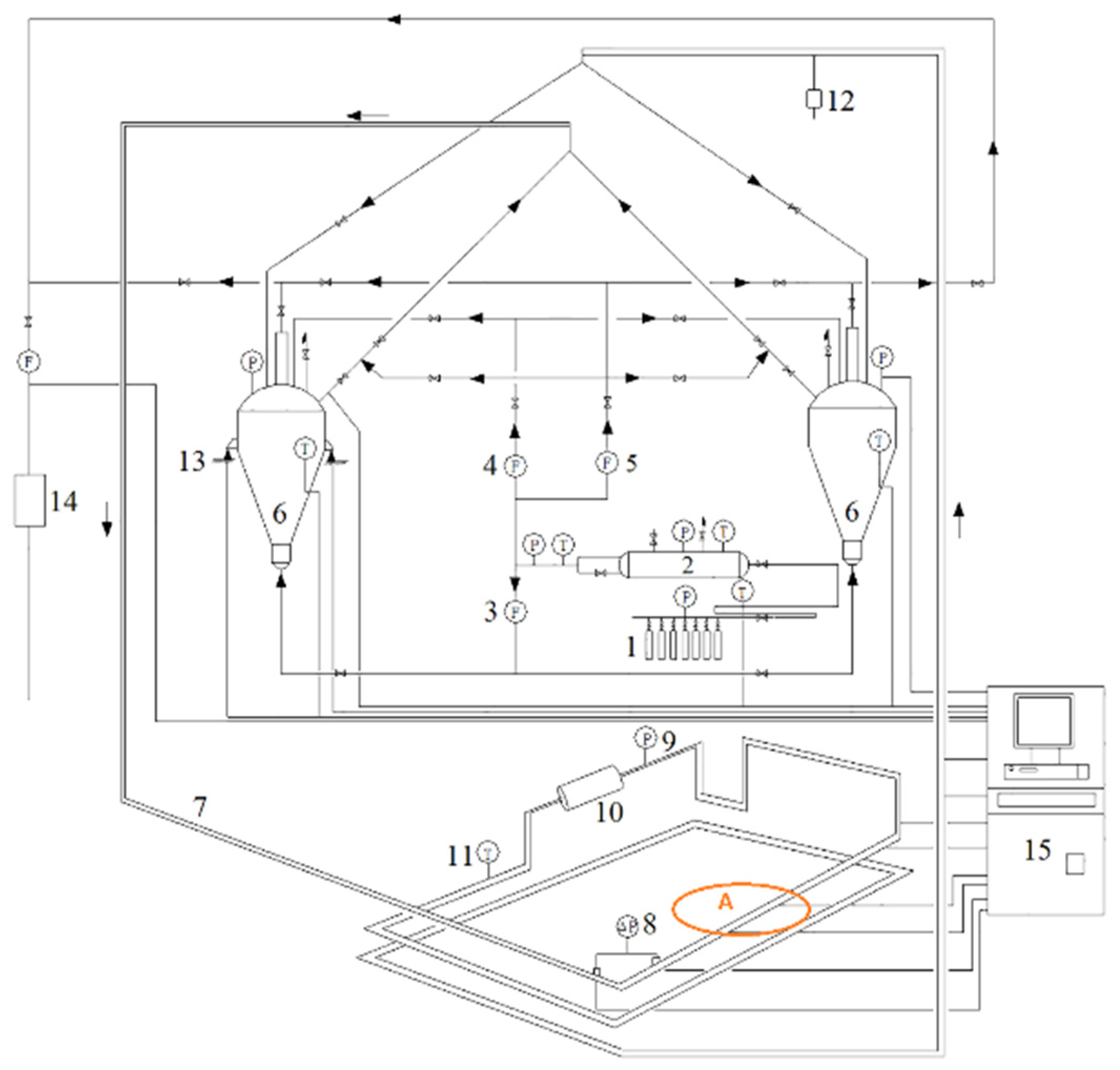
2. Experimental Section

This study conducted a series of high-pressure dense-phase pneumatic conveying experiments using the self-developed-top-discharge-high-pressure-dense-phase pneumatic conveying system [12] from Southeast University, with nitrogen (N₂) as the carrier gas and Inner Mongolian pulverized coal as the conveying material [1]. The whole experimental system, depicted in Figure 1, consists of five main components: the gas supply system, the hoppers, the pipeline, the sensors, and the data sampling and controlling system. During the conveying process, the pressure in the sending hopper (P₁) was maintained at 3.0 MPa, the pressure in the receiving hopper (P₂) was kept at 2.5 MPa, the flow rate of fluidizing gas (Q_f) was held at 0.4 m³/h, and the flow rate of supplementary gas (Q_s) was varied from 0.4 to 1.2 m³/h for the conveying experiment to obtain experimental data (refer to

Table 1. Conveying experiment parameters.

Number	Qs (m3/h)	Ug (m/s)	Ms (kg/s)	αs,inlet	us,inlet (m/s)	Pout (MPa)
1	0.40	4.71	0.213	0.318	4.43	2.91
2	0.60	5.62	0.206	0.286	5.30	2.91
3	0.80	6.43	0.194	0.245	6.09	2.92
4	1.00	7.24	0.181	0.199	6.79	2.93
5	1.20	8.10	0.168	0.184	7.72	2.93

). More detailed information about the whole experimental system is available in references [8,37].

3. Numerical Model

3.1. Basic Governing Equations

The basic governing equations are closed by introducing reasonable constitutive equations based on the two-fluid model (see

Table 2. Basic governing equations of the present two-fluid model.

Items	Phase	Formula
Continuity equations	Gas and Solids	$\frac{\partial }{\partial t}({\alpha }_i{\rho }_i)+\nabla \cdot ({\alpha }_i{\rho }_i{v}_i)=0,{\displaystyle \sum {\alpha }_i}=1$ where i = s for the solids phase and i = g for the gas phase.
Momentum equations	Gas	$\frac{\partial }{\partial t}({\alpha }_g{\rho }_g{v}_g)+\nabla \cdot ({\alpha }_g{\rho }_g{v}_g{v}_g)=-{\alpha }_g\nabla p_g+\nabla \cdot {\sigma }_g-F_{sg}+{\alpha }_g{\rho }_{g}g$
	Solids	$\frac{\partial }{\partial t}({\alpha }_s{\rho }_s{v}_s)+\nabla \cdot ({\alpha }_s{\rho }_s{v}_s{v}_s)=-{\alpha }_s\nabla p_g+\nabla \cdot {\sigma }_s+F_{sg}+{\alpha }_s{\rho }_{s}g$

).

Where σ_g and σ_s being the stress tensors of the gas phase and solids phase, respectively.

$${\sigma }_g={\alpha }_g{\mu }_{g,eff}[\nabla v_g+{(\nabla {\mathit{v}}_g)}^{\mathrm{T}}]+{\alpha }_g({\lambda }_g-\frac{2}{3}{\mu }_{g,eff})(\nabla \cdot {\mathit{v}}_g)I$$

(1)

$$\begin{array}{l}{\mu }_{g,eff}={\mu }_g+{\mu }_{g,t}\\ {\mu }_{g,t}={\rho }_g{C}_{\mu }\frac{k_g^2}{{\epsilon }_g}\end{array}$$

(2)

where μ_g is the gas viscosity, Pa·s; μ_g,t is the gas turbulent viscosity, Pa·s; μ_g,eff is the effective gas viscosity, Pa·s; k_g is the gas turbulent kinetic energy, J; ε_g is the gas turbulent dissipation rate; and C_μ is the turbulence model parameter.

$${\sigma }_s=(-p_s+{\alpha }_s{\lambda }_s(\nabla \cdot v_s))I+2{\alpha }_s{\mu }_{s,eff}{S}_s$$

(3)

$$\begin{array}{l}{\mu }_{s,eff}={\mu }_s+{\mu }_{s,t}\\ S_s=\frac{1}{2}(\nabla v_s+{(\nabla v_s)}^T)-\frac{1}{3}\left(\nabla \cdot v_s\right)I\end{array}$$

(4)

where p_s is the solids pressure, Pa; μ_s is the solids viscosity Pa·s; μ_s,t is the solids turbulent viscosity, Pa·s; μ_s,eff is the effective solids viscosity Pa·s; λ_s is the solids bulk viscosity, Pa·s; S_s is the deviatoric part of strain tensor rate.

3.2. Turbulence Model

The realizable k-ε-k_p-ε_p turbulence model is introduced to simulate the turbulence effects of gas–solid flow in high-pressure dense-phase pneumatic conveying in horizontal pipe.

Gas phase turbulent transport equation:

$$\begin{array}{l}\frac{\partial }{\partial t}({\alpha }_g{\rho }_g{k}_g)+\nabla \cdot ({\alpha }_g{\rho }_g{\mathit{u}}_g{k}_g)=\nabla \cdot \left[{\alpha }_g\left({\mu }_g+\frac{{\mu }_{g,t}}{{\sigma }_k}\right)\nabla k_g\right]+({\alpha }_g{G}_{k,g}-{\alpha }_g{\rho }_g{\epsilon }_g)\\ +\beta (C_{sg}{k}_s-C_{gs}{k}_g)-\beta ({\mathit{u}}_s-{\mathit{u}}_g)\frac{{\mu }_{s,t}}{{\alpha }_s{\sigma }_k}\nabla {\alpha }_s+\beta ({\mathit{u}}_s-{\mathit{u}}_g)\frac{{\mu }_{g,t}}{{\alpha }_g{\sigma }_k}\nabla {\alpha }_g\end{array}$$

(5)

$$\begin{array}{l}\frac{\partial }{\partial t}({\alpha }_g{\rho }_g{\epsilon }_g)+\nabla \cdot ({\alpha }_g{\rho }_g{\mathit{u}}_g{\epsilon }_g)=\nabla \cdot \left[{\alpha }_g\left({\mu }_g+\frac{{\mu }_{g,t}}{{\sigma }_{\epsilon }}\right)\nabla {\epsilon }_g\right]\\ +C_{g\epsilon }{\alpha }_g{\rho }_g{D}_g{\epsilon }_g-C_{1\epsilon }{\alpha }_g{\rho }_g\frac{{\epsilon }_g^2}{k_g+\sqrt{\nu {\epsilon }_g}}+C_{2\epsilon }\frac{{\epsilon }_g}{k_g}[\beta (C_{sg}{k}_s-C_{gs}{k}_g)\\ -\beta ({\mathit{u}}_s-{\mathit{u}}_g)\frac{{\mu }_{s,t}}{{\alpha }_s{\sigma }_{\epsilon }}\nabla {\alpha }_s+\beta ({\mathit{u}}_s-{\mathit{u}}_g)\frac{{\mu }_{g,t}}{{\alpha }_g{\sigma }_{\epsilon }}\nabla {\alpha }_g)]\end{array}$$

(6)

Solids phase turbulent transport equation:

$$\begin{array}{l}\frac{\partial }{\partial t}({\alpha }_s{\rho }_s{k}_s)+\nabla \cdot ({\alpha }_s{\rho }_s{\mathit{u}}_s{k}_s)=\nabla \cdot \left[{\alpha }_s\left({\mu }_s+\frac{{\mu }_{s,t}}{{\sigma }_k}\right)\nabla k_s\right]+({\alpha }_s{G}_{k,s}-{\alpha }_s{\rho }_s{\epsilon }_s)\\ +\beta (C_{gs}{k}_g-C_{sg}{k}_s)-\beta ({\mathit{u}}_g-{\mathit{u}}_s)\frac{{\mu }_{g,t}}{{\alpha }_g{\sigma }_k}\nabla {\alpha }_g+\beta ({\mathit{u}}_g-{\mathit{u}}_s)\frac{{\mu }_{s,t}}{{\alpha }_s{\sigma }_k}\nabla {\alpha }_s\end{array}$$

(7)

$$\begin{array}{l}\frac{\partial }{\partial t}({\alpha }_s{\rho }_s{\epsilon }_s)+\nabla \cdot ({\alpha }_s{\rho }_s{\mathit{u}}_s{\epsilon }_s)=\nabla \cdot \left[{\alpha }_s\left({\mu }_s+\frac{{\mu }_{s,t}}{{\sigma }_{\epsilon }}\right)\nabla {\epsilon }_s\right]\\ +C_{s\epsilon }{D}_s{\alpha }_s{\rho }_s{\epsilon }_s-C_{1\epsilon }{\alpha }_s{\rho }_s\frac{{\epsilon }_s^2}{k_s+\sqrt{\nu {\epsilon }_s}}+C_{2\epsilon }\frac{{\epsilon }_s}{k_s}[\beta (C_{gs}{k}_g-C_{sg}{k}_s)\\ -\beta ({\mathit{u}}_g-{\mathit{u}}_s)\frac{{\mu }_{g,t}}{{\alpha }_g{\sigma }_{\epsilon }}\nabla {\alpha }_g+\beta ({\mathit{u}}_g-{\mathit{u}}_s)\frac{{\mu }_{s,t}}{{\alpha }_s{\sigma }_{\epsilon }}\nabla {\alpha }_s)]\end{array}$$

(8)

Among them, u_g, u_s are the average velocities of gas phase and solids phase, m/s; G_k,g, G_k,s are the turbulent kinetic energy generation terms caused by the average velocities of gas phase and solids phase, respectively. β is the drag coefficient; σ_k and σ_ε are the Prandtl numbers of the turbulent kinetic energy k and the turbulent dissipation rate ε, respectively.

3.3. Three-Zone Drag Model

Given that high-pressure dense-phase pneumatic conveying in horizontal pipe is a non-uniform structured flow composed of three flow regimes (dilute regime, intermediate regime, and dense regime) [8], this study restructured a three-zone drag model (see Equation (9)), which it combined with the advantages of the Huilin–Gidaspow drag model [40] and Mckeen drag model [41]. In this drag model, the Wen and Yu drag model [42] is applied to simulate the dilute regime, the Mckeen drag model is used to simulate the intermediate regime, and the Ergun drag model is utilized to simulate the dense regime.

$${\beta }_{Three-Zone}=\{\begin{array}{l}150\frac{{\alpha }_s\left(1-{\alpha }_g\right){\mu }_g}{{\alpha }_g{d}_s^2}+1.75\frac{{\rho }_g{\alpha }_s}{d_s}\left|{\mathit{v}}_s-{\mathit{v}}_g\right|\hspace{1em}{\alpha }_g<0.6\\ C\left(\frac{17.3}{R{e}_s}+0.336\right)\frac{{\alpha }_s{\rho }_g\left|{\mathit{v}}_s-{\mathit{v}}_g\right|}{d_s}{\alpha }_g^{-1.8}\hspace{1em}0.6\le {\alpha }_g<0.9\\ \frac{3}{4}{C}_D\frac{{\alpha }_s{\alpha }_g{\rho }_g\left|v_s-v_g\right|}{d_s}{\alpha }_g^{-2.65}\hspace{1em}\hspace{1em}\hspace{1em}\hspace{1em}\hspace{1em}{\alpha }_g\ge 0.9\end{array}$$

(9)

$$C_D=\{\begin{array}{l}\frac{24}{R{e}_s}\left[1+0.15{\left(R{e}_s\right)}^{0.687}\right]\hspace{1em}R{e}_s<1000\\ 0.44 R{e}_s\ge 1000\end{array},\hspace{1em}R{e}_s=\frac{{\alpha }_g{\rho }_g{d}_s\left|{\mathit{v}}_s-{\mathit{v}}_g\right|}{{\mu }_g}$$

(10)

$$F_{sg}=\beta \left(v_g-v_{\mathrm{s}}\right)$$

(11)

F_sg is the drag force between the gas and solids phases, Pa. β is the drag coefficient between the gas and solids phases, v_g, v_s are the velocity vectors of the gas and solids phases, m/s.

3.4. Solids Stress Model

3.4.1. Kinetic Theory of Granular Flow

In high-pressure dense-phase pneumatic conveying, it is necessary to consider the solids stress, including interparticle collisions and friction. The two-fluid model commonly employs the kinetic theory of granular flow (KTGF) to simulate particle collisions, and the basic parameter settings for KTGF are provided in

Table 3. Parameter settings of KTGF.

Parameters	Setting
Granular viscosity	Gidaspow [43]
Granular bulk viscosity	Lun et al. [44]
Solids pressure	Lun et al. [44]
Granular conductivity	Gidaspow [43]

. It is well-known that the classical kinetic theory of granular flow is based on the assumption that interparticle collisions occur randomly as instantaneous collisions, and it is therefore only suitable for dilute-phase flow. Therefore, this research introduces Savage radial distribution function g_0,ss to modify the classical KTGF and extend it to the field of dense-phase flow. Lee et al. [26] have also confirmed the reliability of this approach.

$$g_{0,ss}=\frac{1-7{\alpha }_s/16}{{\left(1-{\alpha }_s/{\alpha }_{s,\max }\right)}^2}$$

(12)

where α_s,max is the maximum solids volume fraction for the packing state, whose value is very close to the solids volume fraction of tap density. For pulverized coal, α_s,max ≈ 0.63.

3.4.2. Frictional Stress

Frictional stress is one of the most significant interparticle forces in dense gas–solid flow, revealing the fundamental properties of such flows from a mechanical perspective. A comprehensive frictional stress model comprises both frictional pressure and frictional viscosity. In general, different yield criterions can be employed to develop the corresponding frictional stress model.

For instance, Dartevelle introduced the Pitman–Schaeffer–Gray–Stiles yield criterion to develop the Dartevelle frictional stress model [25]. Compared to conventional frictional stress models, this model simultaneously accounts for both the dilatancy and consolidation of the solids phase in dense-phase gas–solid flow [31].

Dartevelle frictional stress model [25]:

$$p_f=\{\begin{array}{c}1000\frac{{({\alpha }_s-{\alpha }_{s,\min })}^3}{{({\alpha }_{s,\max }-{\alpha }_s)}^3}\hspace{0.17em}\hspace{0.17em}\hspace{0.17em}\hspace{0.17em}\hspace{0.17em}\hspace{0.17em}\hspace{0.17em}\hspace{0.17em}\hspace{0.17em}\hspace{0.17em}\hspace{1em}{\alpha }_{s,\min }<{\alpha }_s<{\alpha }_{s,\max }\\ 0\hspace{0.17em}\hspace{0.17em}\hspace{0.17em}\hspace{0.17em}\hspace{0.17em}\hspace{0.17em}\hspace{0.17em}\hspace{0.17em}\hspace{0.17em}\hspace{0.17em}\hspace{0.17em}\hspace{0.17em}\hspace{0.17em}\hspace{0.17em}\hspace{0.17em}\hspace{0.17em}\hspace{0.17em}\hspace{0.17em}\hspace{0.17em}\hspace{0.17em}\hspace{0.17em}{\alpha }_s\le {\alpha }_{s,\min }\end{array}$$

(13)

$${\mu }_f=\frac{p_f{\sin }^2{\varphi }_i}{\sqrt{2{\sin }^2{\varphi }_i\left(S_s:S_s+{\Theta }_s/d_s^2\right)+{\left(\nabla \cdot v_s\right)}^2}}$$

(14)

Srivastava and Sundaresan [33] introduced the extended von Mises/Coulomb yield criterion, incorporating the fluctuation strain rate term Θ_s/d_s² proposed by Savage to modify and improve the Johnson and Jackson frictional pressure model and Schaeffer frictional viscosity. As a result, the Srivastava and Sundaresan frictional stress model was obtained.

Srivastava and Sundaresan frictional stress model [33]:

$$p_c=\{\begin{array}{c}Fr\frac{{({\alpha }_s-{\alpha }_{s,\min })}^r}{{({\alpha }_{s,\max }-{\alpha }_s)}^s}\hspace{0.17em}\hspace{0.17em}\hspace{0.17em}\hspace{0.17em}\hspace{0.17em}\hspace{0.17em}\hspace{0.17em}\hspace{0.17em}\hspace{0.17em}{\alpha }_{s,\min }<{\alpha }_s<{\alpha }_{s,\max }\\ 0\hspace{0.17em}\hspace{0.17em}\hspace{0.17em}\hspace{0.17em}\hspace{0.17em}\hspace{0.17em}\hspace{0.17em}\hspace{0.17em}\hspace{0.17em}\hspace{0.17em}\hspace{0.17em}\hspace{0.17em}\hspace{0.17em}\hspace{0.17em}\hspace{0.17em}\hspace{0.17em}\hspace{0.17em}\hspace{0.17em}\hspace{0.17em}\hspace{0.17em}\hspace{0.17em}{\alpha }_s\le {\alpha }_{s,\min }\end{array}$$

(15)

$$p_f={\left[1-\frac{\nabla \cdot v_s}{\sqrt{2}n\sin {\varphi }_i\sqrt{S_s:S_s+{\Theta }_s/d_s^2}}\right]}^{n-1}{p}_c$$

(16)

$${\mu }_f=\frac{p_f\sin {\varphi }_{\mathrm{i}}}{\sqrt{2}\sqrt{S_s:S_s+{\Theta }_s/d_s^2}}\left\{n-(n-1){(\frac{p_f}{p_c})}^{\frac{1}{n-1}}\right\}$$

(17)

The coefficient ‘n’ in the above equation mainly depends on the state of the solids phase. When the solids phase expands, i.e., ∇∙v > 0, n = √3/(2sinϕ_i); when the solids phase compresses, i.e., ∇∙v < 0, n = 1.03. Therefore, the Srivastava and Sundaresan frictional stress model considers both the expansion and compression characteristics of the solids phase.

A frictional pressure model is usually obtained by fitting material properties to experimental data. For example, Johnson and Jackson, Syamlal et al., and Chialvo et al. [45] have developed frictional pressure models based on the physical properties of glass beads with different diameters. The Dartevelle frictional pressure model suggests that frictional pressure is only dependent on the solids volume fraction, which is obviously not comprehensive. Although the Johnson and Jackson frictional pressure model introduced three empirical constants (Fr, r, s) to characterize material frictional properties, it did not propose a method for determining these constants. Therefore, in general, these empirical constants (Fr, r, s) need to be adjusted based on simulation results. This not only increases the computational cost but also affects the accuracy, reliability, and applicability of the simulations.

To address these issues, Berzi et al. [46] incorporated two material property parameters, particle stiffness k_n and particle diameter d_s, into the frictional pressure model. They also introduced a constant coefficient ‘a’, which is related to material properties, leading to the development of the Berzi frictional pressure model. Compared to other frictional pressure models, the Berzi frictional pressure model explicitly establishes the relationship between frictional pressure and particle properties. It has certain advantages in investigating the gas–solid flow with different frictional properties. Although this frictional pressure model is not widely used, it is imperative to incorporate particle properties to modify and improve frictional stress models. Therefore, in this study, the modified Berzi frictional stress model, combined with the extended von Mises/Coulomb yield criterion, was established by incorporating the material parameters (stiffness k_n and diameter d_s) of pulverized coal.

The modified Berzi frictional stress model [46]:

$$p_f=f_0\frac{k_n}{d_s},f_0=\{\begin{array}{c}a\frac{{\alpha }_s-{\alpha }_{s,\min }}{{\alpha }_{s,\max }-{\alpha }_s}\hspace{0.17em}\hspace{0.17em}\hspace{0.17em}\hspace{0.17em}\hspace{0.17em}\hspace{0.17em}\hspace{0.17em}\hspace{0.17em}\hspace{0.17em}\hspace{0.17em}\hspace{0.17em}{\alpha }_{s,\min }<{\alpha }_s<{\alpha }_{s,\max }\\ 0\hspace{0.17em}\hspace{0.17em}\hspace{0.17em}\hspace{0.17em}\hspace{0.17em}\hspace{0.17em}\hspace{0.17em}\hspace{0.17em}\hspace{0.17em}\hspace{0.17em}\hspace{0.17em}\hspace{0.17em}\hspace{0.17em}\hspace{0.17em}\hspace{0.17em}\hspace{0.17em}\hspace{0.17em}\hspace{0.17em}\hspace{0.17em}\hspace{0.17em}\hspace{0.17em}{\alpha }_s\le {\alpha }_{s,\min }\end{array}$$

(18)

$${\mu }_f=\frac{p_f{\sin }^2{\varphi }_i}{\sqrt{2{\sin }^2{\varphi }_i\left(S_s:S_s+{\Theta }_s/d_s^2\right)+{\left(\nabla \cdot v_s\right)}^2}}$$

(19)

This study will examine and assess the predictive performance of three frictional stress models, namely Dartevelle frictional stress model, Srivastava and Sundaresan frictional stress model, and the modified Berzi frictional stress model, in the simulation of high-pressure dense-phase pneumatic conveying in horizontal pipe. The objective is to identify a more reasonable frictional stress model that offers improved accuracy in predicting high-pressure dense-phase pneumatic conveying in horizontal pipe.

3.5. Boundary Conditions and Simulation Settings

3.5.1. Boundary Conditions

(1) Inlet boundary conditions: velocity-inlet.

Gas phase: only considering the axial gas velocity distribution v_{g, inlet(r)}:

$$v_{g,\mathrm{inlet}}(r)=\frac{60}{49}\frac{U_g}{1-{\alpha }_{s,\mathrm{inlet}}}{(1-2r/D)}^{1/7}$$

(20)

where r represents the distance to the center of the inlet cross-section, and D is the pipe diameter.

Solids phase: To facilitate convergence, the same gas and solids velocity distribution are set. The axial solids velocity distribution v_s,inlet(r):

$$v_{s,\mathrm{inlet}}(r)=\frac{60}{49}{u}_{s,\mathrm{inlet}}{(1-2r/D)}^{1/7}$$

(21)

$$u_{s,\mathrm{inlet}}=U_g\left(1-0.68d_s^{0.92}{\rho }_s^{0.5}{\rho }_g^{-0.2}{D}^{-0.54}\right)$$

(22)

$${\alpha }_{s,\mathrm{inlet}}=4M_s/\left({\rho }_s{u}_{s,\mathrm{inlet}}\pi D^2\right)$$

(23)

where Equation (22) is an empirical equation used to calculate u_s,inlet.

(2) Outlet boundary conditions: pressure outlet and the outlet pressure are designated as P_out.

(3) Turbulence settings: hydraulic diameter is set to the pipe diameter, and the turbulent intensities for the gas and solids phases are 10% and 5%, respectively.

(4) Wall boundary conditions.

Gas phase: no-slip.

Solids phase: the modified Schneiderbauer solids wall boundary model.

Schneiderbauer et al. [47] proposed a new solids wall boundary model that not only distinguishes between sliding and non-sliding collisions among particles but also integrates them into a single expression. However, the model fails to consider the frictional shear stress generated by particles sliding on the wall, which is crucial for high-pressure dense-phase pneumatic conveying in horizontal pipe. Accounting for the frictional effects at the wall, a frictional stress term was introduced to modify the Schneiderbauer solids wall boundary model.

The modified shear stress between the solids phase and the wall:

$${\tau }_{sw}=-{\eta }_w{\mu }_w{\alpha }_s{\rho }_s{g}_{0,ss}{\Theta }_{s}erf\left({\overline{u}}_{sw}\right)\frac{u_{sw}}{\left|u_{sw}\right|}-{\mu }_w{p}_f{u}_{sw}/\left|u_{sw}\right|$$

(24)

The pseudo-heat flow of the solids phase at the wall:

$$\begin{array}{l}{q}_w={\tau }_{sw}\cdot u_{sw}-\frac{{\alpha }_s{\rho }_s{g}_{0,ss}{\eta }_w\sqrt{{\Theta }_s}}{\sqrt{2\pi }{\mu }_0^2}\exp \left(-{\overline{u}}_{sw}^2\right)\times \\ \left\{\begin{array}{l}{\mu }_w\left[2{\mu }_w{\left|u_{sw}\right|}^2\left(2{\eta }_w-{\mu }_0\right)+{\Theta }_s\left(14{\mu }_w{\eta }_w-4{\mu }_0\left(1+{\mu }_w\right)-6{\mu }_w{\mu }_0^2{\eta }_w\right)\right]\\ +{\mu }_0^2\sqrt{{\Theta }_s}\exp \left({\overline{u}}_{sw}^2\right)\left[\sqrt{{\Theta }_s}\left(4\left({\eta }_w-1\right)+6{\mu }_w^2{\eta }_w\right)-\sqrt{2\pi }{\mu }_w\left|u_{sw}\right|erf\left({\overline{u}}_{sw}\right)\right]\end{array}\right\}\end{array}$$

(25)

$${\eta }_w=\frac{1}{2}\left(1+e_{sw}\right),{\mu }_0=\frac{7}{2}\frac{1+e_{sw}}{1+{\beta }_0}{\mu }_w,{\overline{u}}_{sw}=\frac{u_{sw}}{\sqrt{2{\Theta }_s}{\mu }_0},erf\left(x\right)=\frac{2}{\sqrt{\pi }}{\displaystyle {\int }_0^x\exp \left(-{\xi }^2\right)}d\xi$$

(26)

3.5.2. Simulation Settings

During the computational process, the time step is set to 5 × 10⁻⁵ s, with 40 iterations performed at each time step. The convergence residuals are specified to be 10⁻⁴. And the settings of other relevant mathematical model parameters can refer to

Table 4. Mathematical model parameter setting.

αs,min	αs,max	ess	ϕi	esw	μw	β0	a
0.4	0.63	0.7	32.0°	0.5	0.5	0.3	1.8 × 10−6

.

It should be noted that this study uses UDF provided by FLUENT to compile the radial distribution function, frictional stress model, velocity distribution function, and drag model, and loads them into the ANSYS FLUENT 2020 software for simulation calculations.

4. Results and Discussion

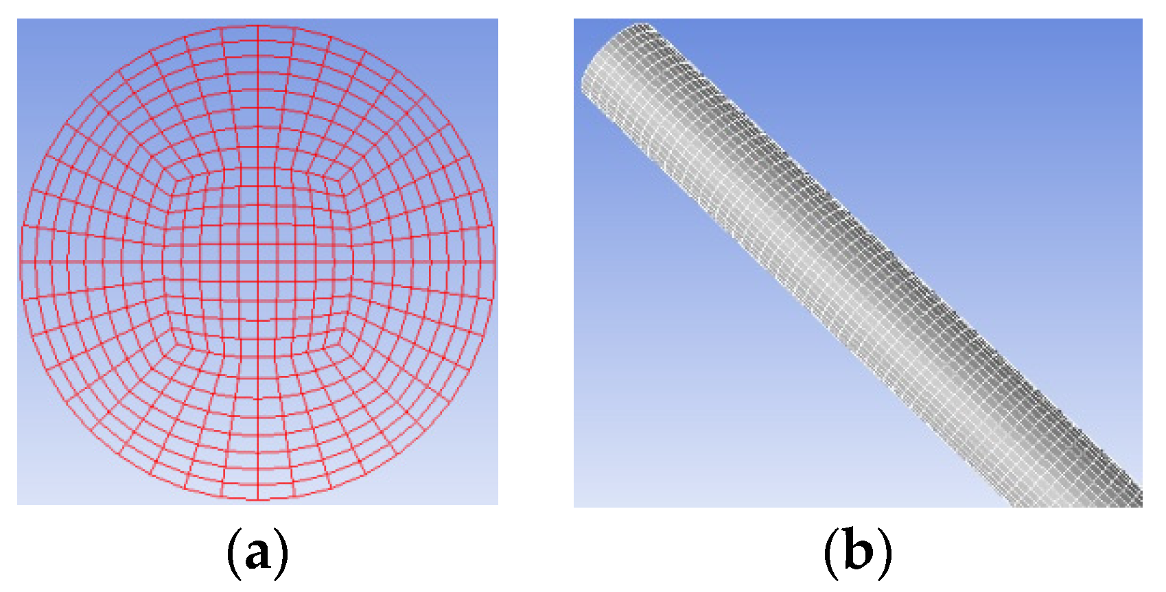
4.1. Grid Division and Its Independence Analysis

As shown in Figure 2, the simulated object is a horizontal pipe (the orange marker A in Figure 1) with a length of 2.4 m, which is meshed by GAMBIT 2.4.6 software.

To enhance the computational accuracy and efficiency of simulation, under typical experimental conditions with supplementary gas Q_s = 0.8 m³/h, the horizontal pipe has been divided into four different mesh specifications (Mesh A, B, C, and D, as illustrated in

Table 5. Predicted pressure drop in horizontal pipe with different mesh specifications.

Mesh Specifications	Inlet Grid Number	Axial Grid Size (mm)	Total Grid Number	Simulated Pressure Drop (kPa)	Experimental Pressure Drop (kPa)
Mesh A	180	2	216,000	3.77	4.26
Mesh B	288	1.5	460,800	3.91
Mesh C	420	1.25	806,400	4.06
Mesh D	576	1	1,382,400	4.09

). Furthermore, the simulation has been conducted using the modified Berzi frictional stress model to investigate mesh-independent boundaries and determine appropriate mesh sizes.

In Table 5, it can be observed that as the grid size decreases, the simulated pressure drop in horizontal pipe gradually converges toward the experimental value. Particularly, when the total number of grids exceeds 460, 800 (e.g., Mesh C and Mesh D), the simulated pressure drop in the horizontal pipe reaches a near-constant state. Mesh C was therefore ultimately selected as the mesh type for simulation calculations.

4.2. Boundary Conditions and Simulation Settings

4.2.1. Pressure Drop in Horizontal Pipe

Figure 3 presents a comparison between the predicted pressure drop in horizontal pipe by using the three frictional stress models and the corresponding experimental data for different supplementary gases. By comparing the simulation results with the experimental data in the figure, it can be observed that the predictions of the pressure drop in horizontal pipe by frictional stress models are highly accurate, with a relative error ranging from −4.91% to +7.60%. Additionally, as the supplementary gas increases, both the simulation results and the experimental data exhibit the same trend of the pressure drop in horizontal pipe initially decreasing and then increasing. Hence, it can be concluded that the three frictional stress models have provided accurate predictions of both the pressure drop in horizontal pipe and its variation with the increase of supplementary gas.

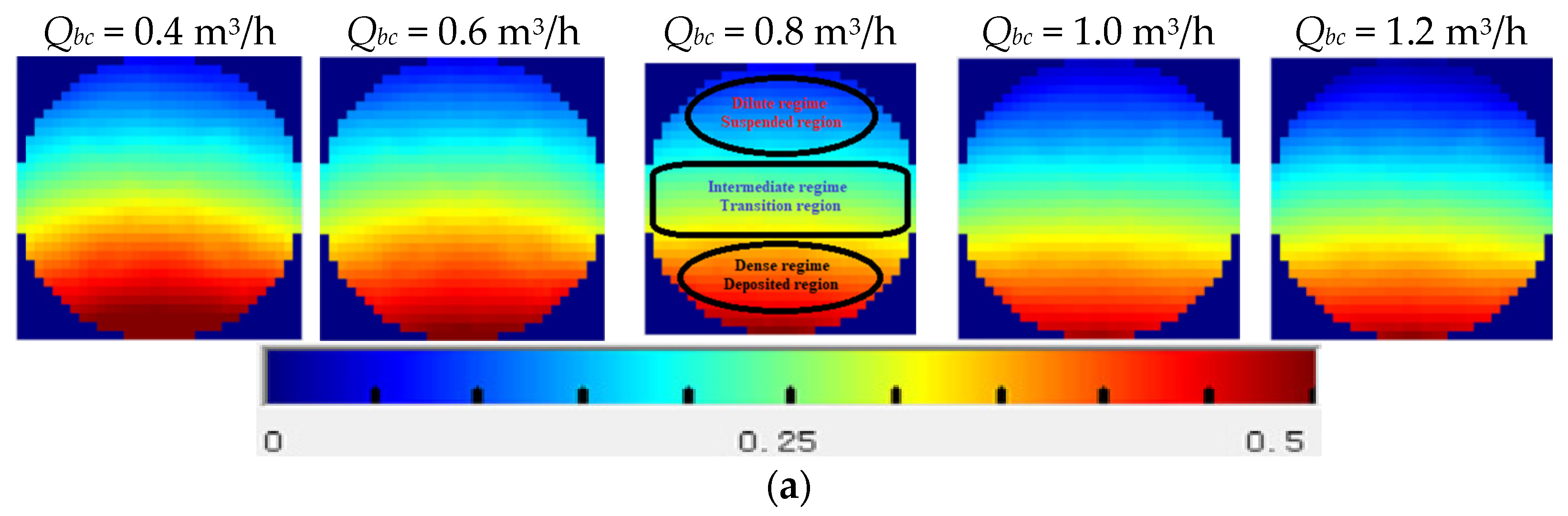
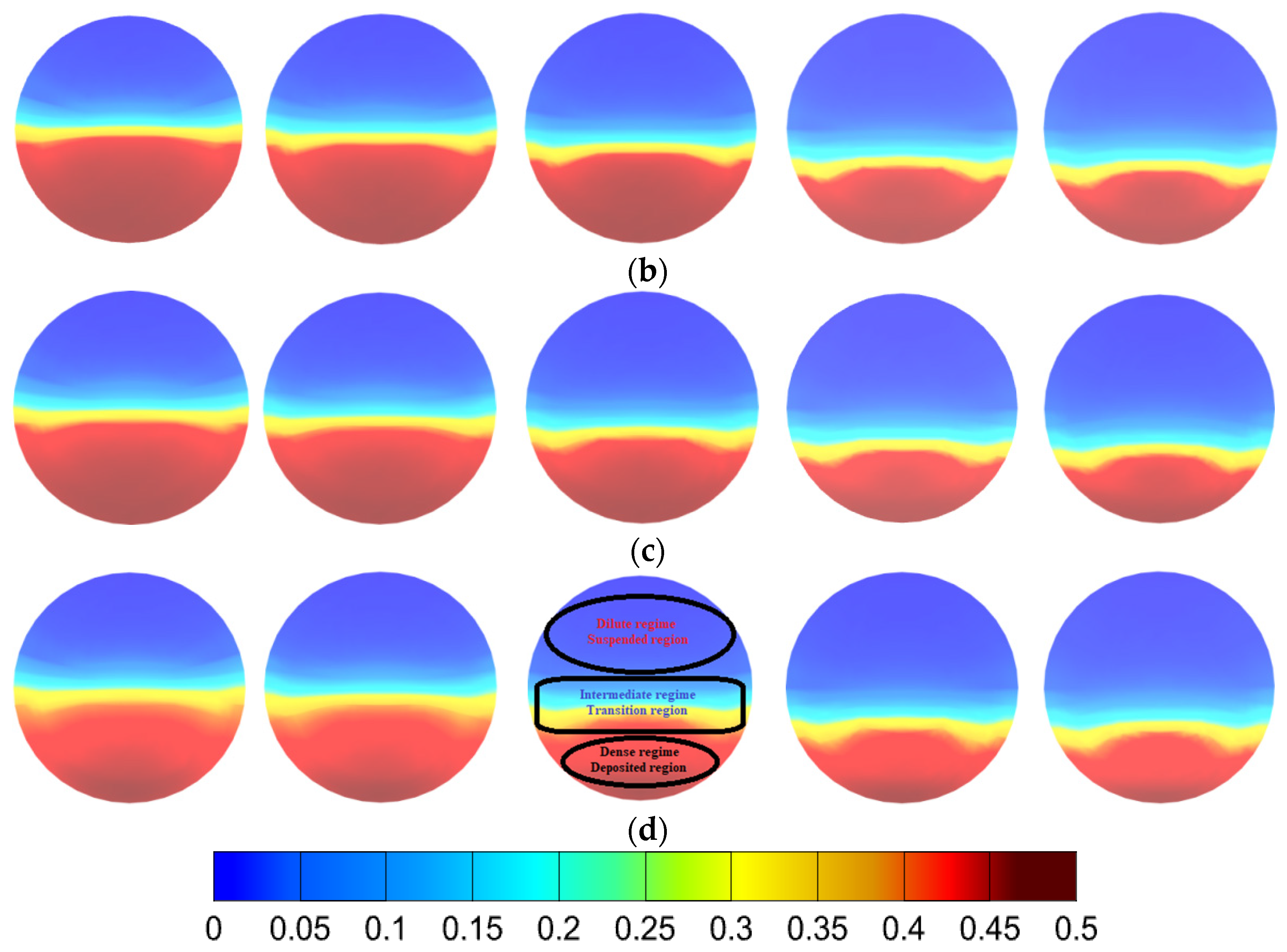
4.2.2. Solids Volume Fraction Distribution

Figure 4 illustrates the distribution of the conveying parameters (gas velocity and solids velocity) along the height of the horizontal pipe in various cross-sections, under a typical experimental condition with Q_s = 0.8 m³/h, using the modified Berzi frictional stress model. It can be observed from the figure that the conveying parameters gradually stabilize along the axial direction of the horizontal pipe. In referring to Figure 4a,b, we see the conveying parameters have already stabilized from the section at L = 120 D (where L represents the distance between the selected section and the inlet section of the pipe, and D represents the pipe diameter). This indicates that the gas–solid flow in horizontal pipe has achieved sufficient development and entered the fully developed section. To investigate the conveying characteristics of high-pressure dense-phase pneumatic conveying in horizontal pipe, this study will discuss the conveying characteristic parameters at the section L = 180 D.

Figure 5 illustrates the comparative relationship between the predicted solids volume fraction distribution contours by using the three frictional stress models and the ECT images. By comparing Figure 5a–d, it is evident that the simulation results generally agree with the corresponding experimental data. The solids volume fraction distribution in the entire horizontal pipe can be categorized into three regions: the upper suspended region corresponding to dilute-phase flow, the middle transition region corresponding to intermediate flow, and the bottom deposited region corresponding to dense-phase flow. However, the boundaries between these regions are not clearly defined. Figure 5 shows that the predicted variations of the deposited region with supplementary gas are fundamentally consistent in horizontal pipe when the three frictional stress models are used, which is also consistent with the variations of the deposited region shown in the ECT images, and namely the bottom deposited region decreasing with increasing supplementary gas. This strongly validates the high reliability of the frictional stress model used in this study.

4.3. Influence of the Frictional Stress Model on the Conveying Characteristics of High-Pressure Dense-Phase Pneumatic Conveying in Horizontal Pipe

The frictional pressure p_f represents the normal stress originating in interparticle continuous contact or compression, and its main function is to prevent an excessive solids volume fraction, which lacks physical significance. Obviously, it is closely related to the solids volume fraction and directly affects the solids volume fraction distribution.

Measurement results indicate that the bulk packing volume fraction α_b is approximately 0.5 for pulverized coal. In this circumstance, the frictional pressure is generated by the weight of the pulverized coal itself. Given that granular flows need the corresponding relative motion space, the solids volume fraction does not generally exceed the bulk packing volume fraction (as shown in Figure 6). Schneiderbauer et al. [48] stated that when α_s ≥ 0.4, it falls into dense-phase flow, and the particles gradually experience compression and frictional effects. Therefore, this study sets α_s,min at 0.4.

Figure 7 illustrates the relationship between the frictional pressure and the solids volume fraction, showing that the frictional pressure increases as the solids volume fraction α_s increases. When the solids volume fraction is below 0.43, Johnson & Jackson frictional pressure is the smallest and exhibits the slowest growth rate, while Berzi frictional pressure is the highest initially before its growth rate is eventually surpassed by Dartevelle frictional pressure. When the solids volume fraction is between 0.43 and 0.47, Dartevelle frictional pressure increases rapidly, far exceeding the other two, and its growth rate also becomes the largest. Johnson and Jackson frictional pressure remains the smallest, but its growth rate eventually surpasses Berzi frictional pressure. When the solids volume fraction is between 0.47 and 0.50, Berzi frictional pressure becomes the smallest and exhibits the slowest growth rate, while Dartevelle frictional pressure remains the largest and has the fastest growth rate. Thus, due to the influence of frictional pressure, there are significant differences in the predicted distribution of the solids volume fraction (particularly in the deposited region) in the three frictional stress models (as shown in Figure 5 and Figure 6). In summary, Dartevelle frictional stress model predicts the lowest solids volume fraction and the steepest solids volume fraction gradient in the deposited region of horizontal pipe, while the modified Berzi frictional stress model predicts the highest solids volume fraction and the gentlest solids volume fraction gradient in the deposited region of horizontal pipe. Comparison with the ECT images in Figure 5a shows that the simulation results obtained using the modified Berzi frictional stress model are closer to the experimental data.

Frictional viscosity or shear stress is directly proportional to the frictional pressure and mainly reflects the resistance characteristics or shear resistance characteristics during interparticle sliding motion. As the frictional viscosity or shear stress increases, the resistance to interparticle relative sliding motion increases, resulting in an increase in the work done by frictional stress and an increase in energy dissipation during the conveying process. In other words, the solids frictional pressure loss also increases. Therefore, frictional viscosity or shear stress is one of the most important factors influencing the pressure drop of high-pressure dense-phase pneumatic conveying in horizontal pipe.

Figure 8 and Figure 9 respectively show interparticle frictional pressure p_f and frictional shear stress τ_f obtained through simulation using the three different frictional stress models under varying supplementary gases. From the two figures, it can be observed that frictional stress, including p_f and τ_f, only exists in the bottom deposited region and decreases with increases of supplementary gas. A comparison of Figure 8 and Figure 9 also reveals that while the range of frictional stress obtained using the three frictional stress models is the same, there are certain differences in their distribution.

As previously mentioned, this is because frictional viscosity or shear stress arises in conjunction with frictional pressure and is directly proportional to it, resulting in a similar variation for τ_f and p_f. When the supplementary gas Q_bc ≤ 0.8 m³/h, the gas flow rate in the conveying pipeline is reduced, resulting in a lower superficial gas velocity and more pulverized coal particles being deposited at the bottom of the pipeline. As a result, the influence of frictional stress is stronger, and the differences with various frictional stress models are more prominent (as shown in Figure 8 and Figure 9). Consequently, due to different frictional stress models, there is a larger disparity in the predicted pressure drop in horizontal pipe.

When Q_bc ≤ 0.8 m³/h, the solids volume fraction is higher in the deposited region at the bottom of the horizontal pipe, and it is almost always higher than 0.43 (see Figure 6). At this time, Dartevelle frictional pressure varies most rapidly with the solids volume fraction, and its value is higher than the other two frictional pressure models (refer to Figure 8), as does Dartevelle frictional shear stress (observed in Figure 9). Therefore, Dartevelle frictional stress model predicts the highest pressure drop in horizontal pipe (refer to Figure 4), while the results are reversed for the modified Berzi frictional stress model.

When Q_bc > 0.8 m³/h, the gas flow rate in the conveying pipeline increases rapidly, leading to an increase in superficial gas velocity and a sharp reduction in pulverized coal deposition at the bottom of the pipeline. The solids volume fraction in the deposited region is almost always lower than 0.47. Especially when predicted by Dartevelle frictional stress model, the solids volume fraction is even lower than 0.43 (refer to Figure 6).

Consequently, the influence of frictional stress is significantly weakened, and the difference between various frictional stress models is visibly diminished (as shown in Figure 8 and Figure 9). Therefore, there is a smaller discrepancy in the predicted pressure drop in horizontal pipe, which is due to different frictional stress models. When Q_bc > 0.8 m³/h, the modified Berzi frictional pressure is the highest (refer to Figure 8), and the same applies to frictional shear stress (refer to Figure 9). Hence, the modified Berzi frictional stress model predicts the highest pressure drop in horizontal pipe (refer to Figure 3).

According to Figure 3, the relative error of pressure drop in horizontal pipe decreases gradually with the increase in supplementary gas. As previously discussed, with the increase of supplementary gas, the deposited region shows a continuous reduction, causing a gradual decrease in interparticle friction and a simultaneous increase in interparticle collision. This discrepancy is attributed to the existing frictional stress model insufficiently considering interparticle frictional properties, such as the oversight of particle shape and particle size distribution, influencing the friction stress model. Therefore, as the supplementary gas decreases, the relative error correspondingly increases.

The distribution of various conveying parameters along the height of horizontal pipe is predicted by different frictional stress models. Figure 10 illustrates the typical experimental conditions with the supplementary gas Q_s = 0.8 m³/h. Among the three frictional stress models, Figure 10f clearly shows the difference in the predicted solids volume fraction distribution. It can be inferred from this figure that the trend of the solids volume fraction is inversely related to the frictional pressure, confirming the above conclusion that the solids volume fraction distribution depends on frictional pressure distribution, which is ultimately determined by the mechanical balance in the conveying pipeline. This is also the fundamental reason for the differences in the predicted pressure drop in horizontal pipe that are observed when the three frictional stress models are used.

As mentioned earlier, when Q_s = 0.8 m³/h, the solids volume fraction in the deposited region is higher (as shown in Figure 10f), and the impact of frictional stress is significant. The simulation results demonstrate that the Dartevelle frictional stress model exhibits the strongest effect in the deposited region, resulting in the highest interparticle energy dissipation, and the lowest solids velocity (as shown in Figure 10b). Consequently, the gas–solid interaction intensifies, leading to a decrease in gas velocity, which also becomes the lowest (as shown in Figure 10a).

Additionally, frictional stress hinders interparticle relative movement, resulting in a decrease in solids’ fluctuation velocity. Hence, Dartevelle frictional stress model predicts the lowest solids turbulent kinetic energy (as shown in Figure 10d). Since the solids turbulent kinetic energy has a dominant role, due to the higher solids volume fraction in the deposited region, it also influences the gas turbulent kinetic energy, making it the minimum (as shown in Figure 10c). The particle pseudo-temperature is dependent on the fluctuation intensity of the individual particle. In the high solids volume fraction of the deposited region, the fluctuation of individual particle is limited, resulting in a lower particle pseudo-temperature. Consequently, the Dartevelle frictional stress model, which predicts the lowest solids volume fraction (as shown in Figure 10f), has the highest particle pseudo-temperature (as shown in Figure 10e). The simulation results of the modified Berzi frictional stress model exhibit the opposite trends to the aforementioned results.

Figure 10 shows that the three frictional stress models had almost no impact on the simulation results, due to the dominance of KTGF in the suspended region. However, for the transition region, the simulation results of the three frictional stress models were almost contrary to those of the deposited region. This discrepancy arose from the requirement of maintaining consistency in the gas and solids mass flow rate.

In short, the influence of frictional stress models on the simulation results of high-pressure dense-phase pneumatic conveying in horizontal pipe was mainly observed in the transition and deposited regions. The frictional stress influences other conveying parameters by affecting the solids volume fraction distribution and the pressure drop in horizontal pipe. Through comparative analysis of the simulation results obtained from the three frictional stress models, it was discovered that the simulation results predicted by the modified Berzi frictional stress model closely aligned with the corresponding experimental data. Additionally, this model better characterized the frictional properties of pulverized coal. These findings of the study led us to the conclusion that the modified Berzi frictional stress model provides a more rational approach to predicting frictional stress in high-pressure dense-phase pneumatic conveying in horizontal pipe.

5. Conclusions

Based on the two-fluid model, this study developed a three-zone drag model, modified the classical kinetic theory of granular flows and the Schneiderbauer solids wall boundary condition, and introduced the realizable k-ε-k_p-ε_p turbulent model to establish a three-dimensional unsteady mathematical model for high-pressure dense-phase pneumatic conveying in horizontal pipe. Using this mathematical model, this study proposed to consider the influence of Dartevelle frictional stress model, Srivastava and Sundaresan frictional stress model, and the modified Berzi frictional stress model on the simulation results of high-pressure dense phase pneumatic conveying in horizontal pipe. The main conclusions obtained are as follows:

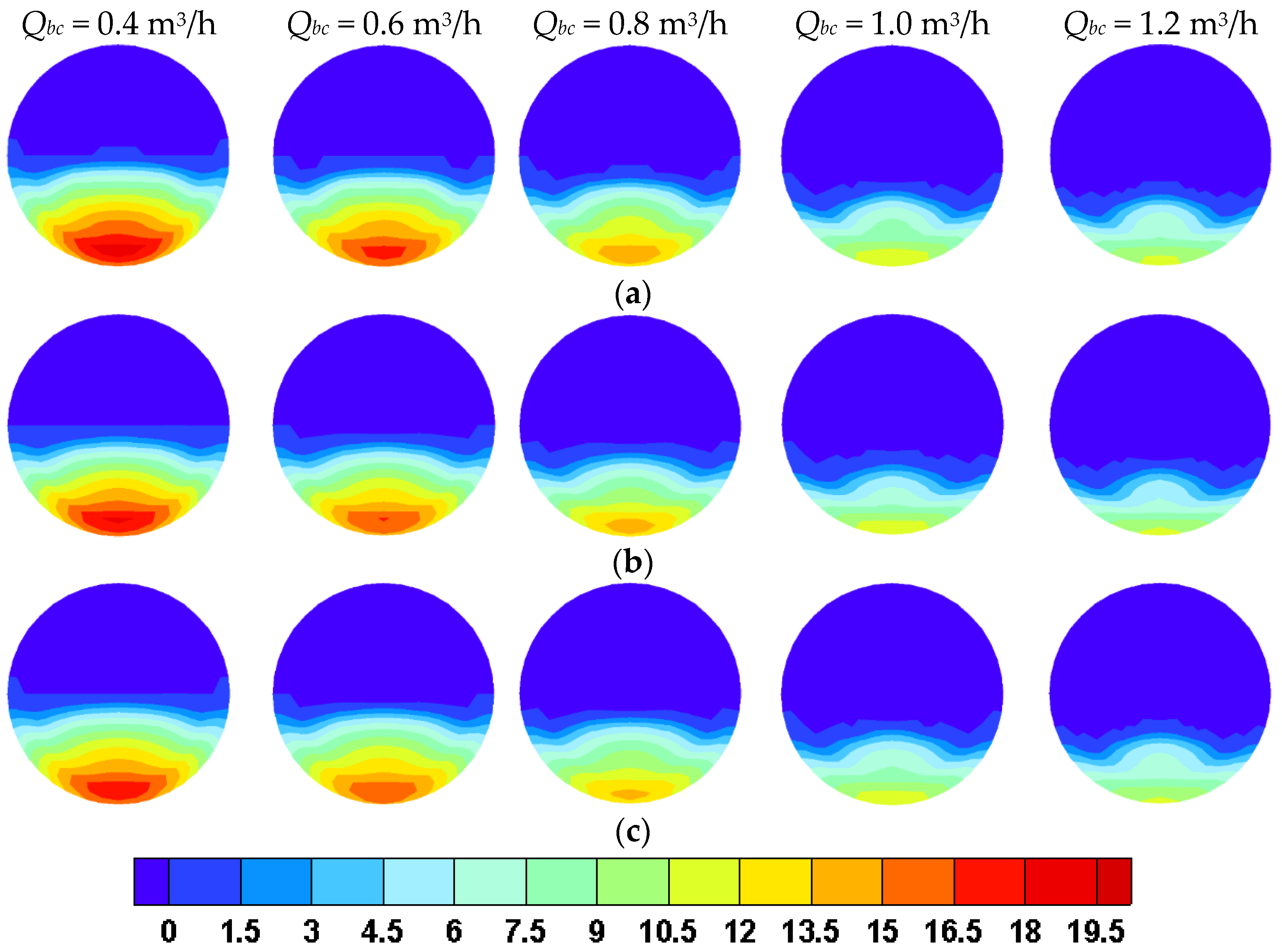
• The predicted pressure drop in horizontal pipe and its variation with supplementary gas are, using the three frictional stress models, seen to be in good agreement with the corresponding experimental data, with relative errors ranging from −4.91% to +7.60%. In addition, the predicted solids volume fraction distribution contours in the three frictional stress models generally agree with the ECT images in the cross-section of the horizontal pipe. In particular, the predicted variations of the deposited region with supplementary gas are also consistent with those in the ECT images.
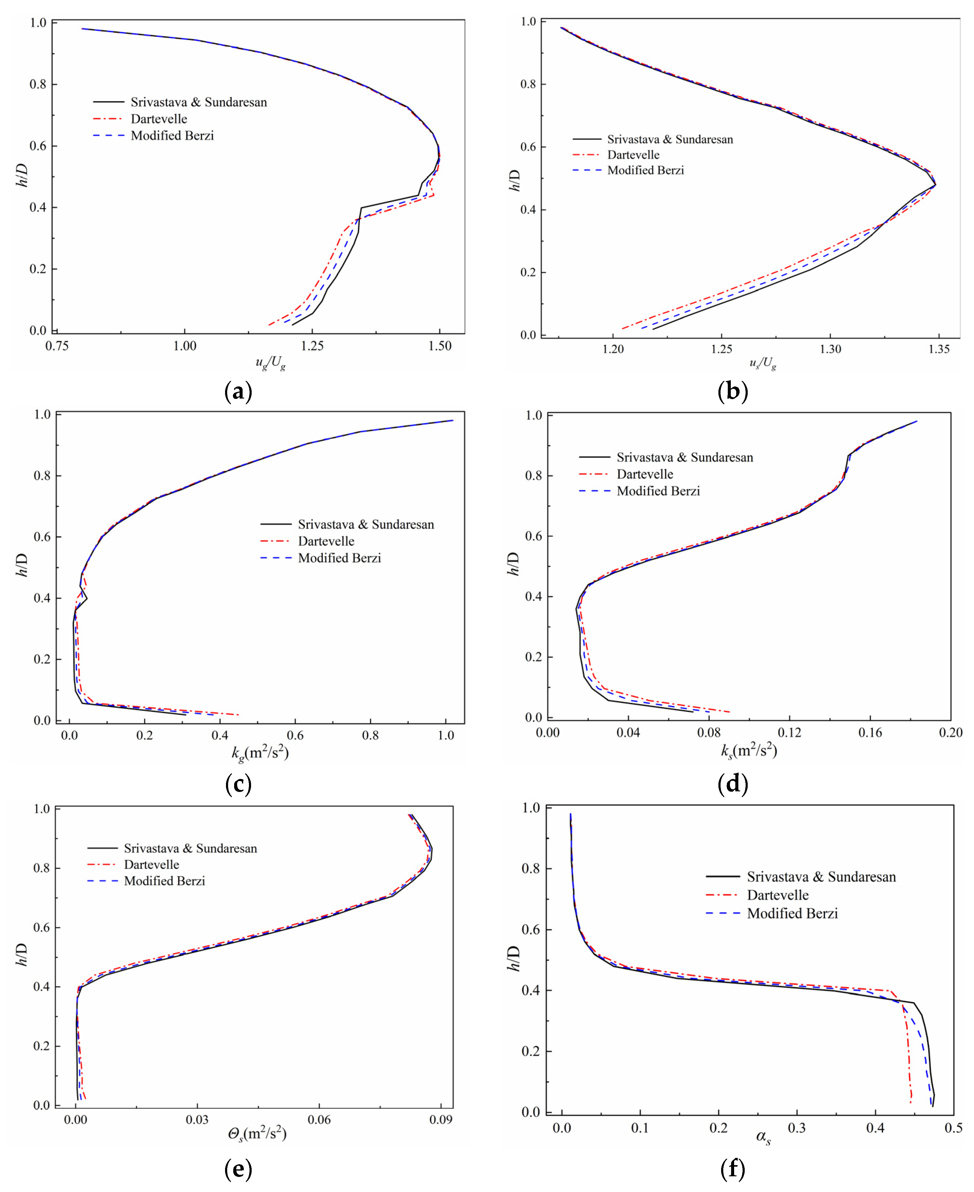
• The effect of frictional stress models on the simulation results of high-pressure dense-phase pneumatic conveying in horizontal pipe only presents in the transition region and deposited region. However, the two regions exhibit opposite changes. Frictional stress only exists in the bottom deposited region and diminishes gradually with the rise in supplementary gas.
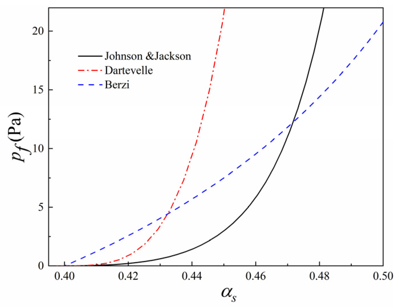
• The three frictional stress models predict a similar variation range of frictional stress, but their distributions differ, which is a fundamental reason for the variations of the solids volume fraction distribution. This also explains the variation of pressure drop in horizontal pipe. The larger the frictional pressure, the lower the solids volume fraction; and the stronger the frictional viscosity or shear stress, the higher the pressure drop in horizontal pipe.
• After comparing the simulation results of the three frictional stress models, it was observed that Dartevelle frictional stress demonstrates the strongest effect and highest energy consumption in the deposited region. Consequently, this leads to the lowest gas and solids velocity, turbulent kinetic energy, and solids volume fraction, and the highest particle pseudo-temperature. However, the simulation results predicted by the modified Berzi frictional stress model exhibit an opposite trend to the above results.
• Among the three frictional stress models, the simulation results of the modified Berzi frictional stress model are more consistent with the experimental data. Additionally, this model better reflects the frictional properties of pulverized coal. In conclusion, the modified Berzi frictional stress model can provide a more accurate prediction of frictional stress in high-pressure dense-phase pneumatic conveying.

References

1. Zhou, H.; Xiong, Y.; Pei, Y. Effect of moisture content on dense-phase pneumatic conveying of pulverized lignite under high pressure. Powder Technol. 2016, 287, 355–363. [Google Scholar] [CrossRef]
2. Klinzing, G.E. A review of pneumatic conveying status, advances and projections. Powder Technol. 2018, 333, 78–90. [Google Scholar] [CrossRef]
3. Lu, P.; Yang, P.; Zheng, X.; Chen, X.; Zhao, C. Pilot-Scale Experimental Study on Phase Diagrams of Pressurized Pneumatic Conveying with Pulverized Coal. Energy Fuel 2017, 31, 10260–10266. [Google Scholar] [CrossRef]
4. Miao, Z.; Kuang, S.; Zughbi, H.; Yu, A. Numerical simulation of dense-phase pneumatic transport of powder in horizontal pipes. Powder Technol. Int. J. Sci. Technol. Wet. Dry. Part. Syst. 2020, 361, 62–73. [Google Scholar] [CrossRef]
5. He, C.; Chen, X.; Wang, J.; Ni, H.; Xu, Y.; Zhou, H.; Xiong, Y.; Shen, X. Conveying characteristics and resistance characteristics in dense phase pneumatic conveying of rice husk and blendings of rice husk and coal at high pressure. Powder Technol. 2012, 227, 51–60. [Google Scholar] [CrossRef]
6. Sun, S.; Yuan, Z.; Peng, Z.; Moghtaderi, B.; Doroodchi, E. Computational investigation of particle flow characteristics in pressurised dense phase pneumatic conveying systems. Powder Technol. 2018, 329, 241–251. [Google Scholar] [CrossRef]
7. Jin, Y.; Lu, H.; Guo, X.; Gong, X. Flow patterns classification of dense-phase pneumatic conveying of pulverized coal in the industrial vertical pipeline. Adv. Powder Technol. 2019, 30, 1277–1289. [Google Scholar] [CrossRef]
8. Zhou, H.; Xiong, Y. Conveying mechanisms of dense-phase pneumatic conveying of pulverized lignite in horizontal pipe under high pressure. Powder Technol. 2020, 363, 7–22. [Google Scholar] [CrossRef]
9. Sharma, A.; Mallick, S.S. An investigation into pressure drop through bends in pneumatic conveying systems. Particul. Sci. Technol. 2021, 39, 180–191. [Google Scholar] [CrossRef]
10. Wang, X.; Luo, B.; You, M.; Liang, C.; Liu, D.; Ma, J.; Chen, X. Experimental and modeling study of gas flow characteristics in the compressible powder bed during gas pressurization. Chem. Eng. Sci. 2023, 268, 118445. [Google Scholar] [CrossRef]
11. Manjula, E.V.P.J.; Ariyaratne, W.K.H.; Ratnayake, C.; Melaaen, M.C. A review of CFD modelling studies on pneumatic conveying and challenges in modelling offshore drill cuttings transport. Powder Technol. 2017, 305, 782–793. [Google Scholar] [CrossRef]
12. Kuang, S.; Zhou, M.; Yu, A. CFD-DEM modelling and simulation of pneumatic conveying: A review. Powder Technol. 2020, 365, 186–207. [Google Scholar] [CrossRef]
13. Sung, W.C.; Kim, J.Y.; Chung, S.W.; Lee, D.H. Effect of particle size distribution on hydrodynamics of pneumatic conveying system based on CPFD simulation. Adv. Powder Technol. 2021, 32, 2336–2344. [Google Scholar] [CrossRef]
14. Zhou, J.; Shangguan, L.; Gao, K.; Wang, Y.; Hao, Y. Numerical study of slug characteristics for coarse particle dense phase pneumatic conveying. Powder Technol. 2021, 392, 438–447. [Google Scholar] [CrossRef]
15. Song, Z.; Li, Q.; Li, F.; Chen, Y.; Ullah, A.; Chen, S.; Wang, W. MP-PIC simulation of dilute-phase pneumatic conveying in a horizontal pipe. Powder Technol. 2022, 410, 117894. [Google Scholar] [CrossRef]
16. Zhao, H.; Zhao, Y. CFD-DEM simulation of pneumatic conveying in a horizontal pipe. Powder Technol. 2020, 373, 58–72. [Google Scholar] [CrossRef]
17. Ariyaratne, W.K.H.; Ratnayake, C.; Melaaen, M.C. Application of the MP-PIC method for predicting pneumatic conveying characteristics of dilute phase flows. Powder Technol. 2017, 310, 318–328. [Google Scholar] [CrossRef]
18. Jin, Y.; Lu, H.; Guo, X.; Gong, X. Application of CPFD method in the simulation of vertical dense phase pneumatic conveying of pulverized coal. Powder Technol. 2019, 357, 343–351. [Google Scholar] [CrossRef]
19. Miao, Z.; Kuang, S.; Zughbi, H.; Yu, A. CFD simulation of dilute-phase pneumatic conveying of powders. Powder Technol. 2019, 349, 70–83. [Google Scholar] [CrossRef]
20. Datta, B.K.; Ratnayaka, C. A Possible Scaling-up Technique for Dense Phase Pneumatic Conveying. Particul. Sci. Technol. 2005, 23, 201–204. [Google Scholar] [CrossRef]
21. Zhong, W.; Zhang, M.; Jin, B.; Yuan, Z. Three-dimensional Simulation of Gas/Solid Flow in Spout-fluid Beds with Kinetic Theory of Granular Flow. Chin. J. Chem. Eng. 2006, 14, 611–617. [Google Scholar] [CrossRef]
22. Ma, A.C.; Williams, K.C.; Zhou, J.M.; Jones, M.G. Numerical study on pressure prediction and its main influence factors in pneumatic conveyors. Chem. Eng. Sci. 2010, 65, 6247–6258. [Google Scholar] [CrossRef]
23. Wang, Y.; Williams, K.; Jones, M.; Chen, B. CFD simulation methodology for gas-solid flow in bypass pneumatic conveying—A review. Appl. Therm. Eng. 2017, 125, 185–208. [Google Scholar] [CrossRef]
24. Tardos, G.I.; McNamara, S.; Talu, I. Slow and intermediate flow of a frictional bulk powder in the Couette geometry. Powder Technol. 2003, 131, 23–39. [Google Scholar] [CrossRef]
25. Dartevelle, S. Numerical modeling of geophysical granular flows: 1. A comprehensive approach to granular rheologies and geophysical multiphase flows. Geochem. Geophys. Geosyst. 2004, 5. [Google Scholar] [CrossRef]
26. Lee, C.; Huang, Z.; Chiew, Y. A three-dimensional continuum model incorporating static and kinetic effects for granular flows with applications to collapse of a two-dimensional granular column. Phys. Fluids 2015, 27, 113303. [Google Scholar] [CrossRef]
27. Jop, P. Rheological properties of dense granular flows. Cr. Phys. 2015, 16, 62–72. [Google Scholar] [CrossRef]
28. Johnson, P.C.; Jackson, R. Frictional–collisional constitutive relations for granular materials, with application to plane shearing. J. Fluid. Mech. 1987, 176, 67–93. [Google Scholar] [CrossRef]
29. Johnson, P.C.; Nott, P.; Jackson, R. Frictional–collisional equations of motion for participate flows and their application to chutes. J. Fluid. Mech. 1990, 210, 501–535. [Google Scholar] [CrossRef]
30. Schaeffer, D.G. Instability in the evolution equations describing incompressible granular flow. J. Differ. Equ. 1987, 66, 19–50. [Google Scholar] [CrossRef]
31. Nikolopoulos, A.; Nikolopoulos, N.; Varveris, N.; Karellas, S.; Grammelis, P.; Kakaras, E. Investigation of proper modeling of very dense granular flows in the recirculation system of CFBs. Particuology 2012, 10, 699–709. [Google Scholar] [CrossRef]
32. Nikolopoulos, A.; Nikolopoulos, N.; Charitos, A.; Grammelis, P.; Kakaras, E.; Bidwe, A.R.; Varela, G. High-resolution 3-D full-loop simulation of a CFB carbonator cold model. Chem. Eng. Sci. 2013, 90, 137–150. [Google Scholar] [CrossRef]
33. Srivastava, A.; Sundaresan, S. Analysis of a frictional–kinetic model for gas–particle flow. Powder Technol. 2003, 129, 72–85. [Google Scholar] [CrossRef]
34. Savage, S.B. Analyses of slow high-concentration flows of granular materials. J. Fluid. Mech. 1998, 377, 1–26. [Google Scholar] [CrossRef]
35. Chen, W.F. The Mechanics of Soils—An Introduction to Critical State Soil Mechanics. Eng. Geol. 1981, 17, 80–81. [Google Scholar] [CrossRef]
36. Ahmadi, G. A generalized continuum theory for granular materials. Int. J. Nonlin. Mech. 1982, 17, 21–33. [Google Scholar] [CrossRef]
37. Pu, W.; Zhao, C.; Xiong, Y.; Liang, C.; Chen, X.; Lu, P.; Fan, C. Numerical simulation on dense phase pneumatic conveying of pulverized coal in horizontal pipe at high pressure. Chem. Eng. Sci. 2010, 65, 2500–2512. [Google Scholar] [CrossRef]
38. Syamlal, M.; Rogers, W.; O’Brien, T.J. MFIX documentation theory guide. In National Technical Information Service; USDOE: Washington, DC, USA, 1993. [Google Scholar] [CrossRef]
39. Wang, Y.; Williams, K.C.; Jones, M.G.; Chen, B. Gas–solid flow behaviour prediction for sand in bypass pneumatic conveying with conventional frictional-kinetic model. Appl. Math. Model. 2016, 40, 9947–9965. [Google Scholar] [CrossRef]
40. Huilin, L.; Gidaspow, D. Hydrodynamics of binary fluidization in a riser: CFD simulation using two granular temperatures. Chem. Eng. 2003, 58, 3777–3792. [Google Scholar] [CrossRef]
41. McKeen, T.; Pugsley, T. Simulation and experimental validation of a freely bubbling bed of FCC catalyst. Powder Technol. 2003, 129, 139–152. [Google Scholar] [CrossRef]
42. Wen, C.Y.; Yu, Y.H. Mechanics of Fluidization. Chem. Eng. Prog. Symp. Ser. 1966, 162, 100–111. [Google Scholar]
43. Gidaspow, D.; Bezburuah, R.; Ding, J. Hydrodynamics of Circulating Fluidized Beds: Kinetic Theory Approach. In Engineering; USDOE: Washington, DC, USA, 1991. [Google Scholar]
44. Lun, C.K.K.; Savage, S.B.; Jeffrey, D.J.; Chepurniy, N. Kinetic theories for granular flow: Inelastic particles in Couette flow and slightly inelastic particles in a general flowfield. J. Fluid. Mech. 1984, 140, 223–256. [Google Scholar] [CrossRef]
45. Chialvo, S.; Sun, J.; Sundaresan, S. Bridging the rheology of granular flows in three regimes. Phys. Rev. E Stat. Nonlin. Soft Matter Phys. 2012, 85, 21305. [Google Scholar] [CrossRef] [PubMed]
46. Berzi, D.; di Prisco, C.G.; Vescovi, D. Constitutive relations for steady, dense granular flows. Phys. Rev. E Stat. Nonlin. Soft Matter Phys. 2011, 84, 31301. [Google Scholar] [CrossRef]
47. Schneiderbauer, S.; Schellander, D.; Löderer, A.; Pirker, S. Non-steady state boundary conditions for collisional granular flows at flat frictional moving walls. Int. J. Multiphas Flow. 2012, 43, 149–156. [Google Scholar] [CrossRef]
48. Soleimani, A.; Schneiderbauer, S.; Pirker, S. A comparison for different wall-boundary conditions for kinetic theory based two-fluid models. Int. J. Multiphas Flow. 2015, 71, 94–97. [Google Scholar] [CrossRef]
Figure 1. Experimental system schematic diagram of dense-phase pneumatic conveying under high pressure. 1. Gas cylinders; 2. Gas buffer tank; 3. Fluidizing gas flowmeter; 4. Pressurizing gas flowmeter; 5. Supplementary gas flow meter; 6. Material storage vessels; 7. Conveying pipeline loop; 8. Differential pressure transmitter; 9. Pressure transducer; 10. Sight-glass section; 11. Temperature sensor; 12. On-line sampler; 13. Load cell; 14. Electric control valve; 15. Control cabinet.
Applsci 14 02031 g001
Figure 2. Grid division of horizontal pipe: (a) Inlet cross-section grids; (b) Pipe wall surface grids.
Applsci 14 02031 g002
Figure 3. Comparative relationship between the predicted pressure drop in horizontal pipe with supplementary gas, using different frictional stress models and the corresponding experimental data.
Applsci 14 02031 g003
Figure 4. Distribution of the conveying parameters along the height of horizontal pipe at various cross-sections. (a) Gas velocity; (b) Solids velocity.
Applsci 14 02031 g004
Figure 5. Comparative relationship between the predicted solids volume fraction distribution contours using three different frictional stress models and ECT images. (a) ECT; (b) Dartevelle frictional stress model; (c) Srivastava and Sundaresan frictional stress model; (d) Modified Berzi frictional stress model.
Applsci 14 02031 g005aApplsci 14 02031 g005b
Figure 6. Solids volume fraction distribution along the height of horizontal pipe simulated by different frictional stress models: (a) Dartevelle frictional stress model; (b) Srivastava and Sundaresan frictional stress model; (c) Modified Berzi frictional stress model.
Applsci 14 02031 g006
Figure 7. Relationship between frictional pressure pf and solids volume fraction.
Applsci 14 02031 g007
Figure 8. Frictional pressure pf predicted by different frictional stress models: (a) Dartevelle frictional stress model; (b) Srivastava and Sundaresan frictional stress model; (c) Modified Berzi frictional stress model.
Applsci 14 02031 g008
Figure 9. Frictional shear stress τf predicted by different frictional stress models: (a) Dartevelle frictional stress model; (b) Srivastava and Sundaresan frictional stress model; (c) Modified Berzi frictional stress model.
Applsci 14 02031 g009
Figure 10. Distribution of conveying parameters along the height of horizontal pipe predicted by different frictional stress models. (a) Gas velocity; (b) Solids velocity; (c) Gas turbulent kinetic energy; (d) Solids turbulent kinetic energy; (e) Particle pseudo-temperature; (f) Solids volume fraction.
Applsci 14 02031 g010