Article

A Novel Spatial–Temporal Deep Learning Method for Metro Flow Prediction Considering External Factors and Periodicity

1
School of Transportation Engineering, Chang’an University, Xi’an 710064, China
2
School of Information Science and Technology, Northwest University, Xi’an 710127, China
3
School of Economy and Management, Chang’an University, Xi’an 710064, China
*
Author to whom correspondence should be addressed.
Appl. Sci. 2024, 14(5), 1949; https://doi.org/10.3390/app14051949
Submission received: 13 January 2024 / Revised: 21 February 2024 / Accepted: 26 February 2024 / Published: 27 February 2024
(This article belongs to the Special Issue Advances in Intelligent Transportation Systems)

Abstract

:
Predicting metro traffic flow is crucial for efficient urban planning and transit management. It enables cities to optimize resource allocation, reduce congestion, and enhance the overall commuter experience in rapidly urbanizing environments. Nevertheless, metro flow prediction is challenging due to the intricate spatial–temporal relationships inherent in the data and the varying influence of external factors. To model spatial–temporal correlations considering external factors, a novel spatial–temporal deep learning framework is proposed in this study. Firstly, mutual information is utilized to select the highly corrected stations of the examined station. Compared with the traditional correlation calculation methods, mutual information is particularly advantageous for analyzing nonlinear metro flow data. Secondly, metro flow data reflecting the historical trends from different time granularities are incorporated. Additionally, the external factor data that influence the metro flow are also considered. Finally, these multiple sources and dimensions of data are combined and fed into the deep neural network to capture the complex correlations of multi-dimensional data. Sufficient experiments are designed and conducted on the real dataset collected from Xi’an subway to verify the effectiveness of the proposed model. Experimental results are comprehensively analyzed according to the POI information around the subway station.

1. Introduction

Urban rail transit is an important means of transportation in modern times. Due to the high cost of opening a new line [1], analysis of passenger flow is helpful to make full use of existing urban rail transit and to improve route planning, so as to improve its efficiency. Therefore, it is particularly important to analyze its passenger flow and predict it.
The main factors affecting the passenger demand include space, time, and semantic factors [2]. From the perspective of space, urban areas can be divided into residential areas, commercial areas, industrial areas, scenic areas, and other functional areas. In different urban functional areas, the distribution of subway stations and the demand for taking subways are different. Passenger demand between areas with similar urban functions is related [3]. In addition, passenger demand between adjacent stations is correlated. If the passenger demand of the first few stations is large, there is a high probability of high passenger demand at the next station [1]. From the perspective of time, subway passenger demand between different stations may change over time. Aside from time and space factors, whether residents choose to take the subway is also subject to a variety of semantic factors, including meteorological factors, traffic control for holidays and special activities, and other factors [4], such as location conditions and textual semantic information [5,6]. Therefore, the difficulty and key point of accurately predicting subway passenger demand is to fuse semantic-rich nonlinear features and dynamically model the spatial–temporal correlation of data.
There are three main types of methods to predict metro flow: statistical methods, traditional machine learning methods, and deep learning methods. To predict metro flow, traditional methods like the simple moving average (MA) [7], autoregressive moving average (ARMA) [7,8], autoregressive integrated moving average (ARIMA), and their variants [7,8,9] are used. For example, Tang et al. used the ARIMA method in terms of varying features, forecasting steps, and forecasting horizons [9]. Nevertheless, metro flow data is usually nonlinear. This means that the linear assumption of these models limits their prediction accuracy.
To understand nonlinear dependencies in metro flow data, researchers have studied machine learning approaches like multilinear regression (MLR) [10], support vector regression (SVR) [9], logistic regression (LR) [11], support vector machines (SVMs) [12,13], decision trees (DTs) [14], the hidden Markov model (HMM) [15], and back propagation neural networks [16]. These methods overcome the limitations of the linear assumption of data. Nevertheless, the traditional machine learning methods often rely on feature extraction and selection, and they can only capture shallow nonlinear dependencies. Predicting traffic accurately is very difficult because we cannot capture detailed patterns in big datasets. This limits the use of accurate metro flow prediction.
Deep learning is a powerful machine learning technique. It has great potential for predicting metro flow [17]. Deep learning can automatically model complex relationships between stations and time intervals. For instance, Xiong et al. proposed a real-time metro flow prediction model using a convolutional neural network (CNN) to predict an urban rail transit passenger flow time series and spatial–temporal series [18]. Recurrent neural networks (RNNs) have emerged as the preferred neural network for temporal dependencies [19]. Nevertheless, traditional RNNs have the problem of gradient disappearance and gradient explosion in long-term prediction. LSTM and GRU networks are special versions of RNNs that solve the gradient problem effectively [20]. GRUs can capture long-term dependencies in sequential data and train the model faster [21]. Shi et al. used a fully connected neural network with short-term memory to predict metro flow [21]. The network was trained using historical metro flow data and meteorological data. Furthermore, there are advanced deep learning approaches like attention mechanism-based methods and semi-supervised deep learning methods [22,23,24]. Xie et al. innovatively built a spatial–temporal dynamic graph relationship learning model [25], and Zhang et al. introduced a spatial–temporal graph GAN for accurate short-term passenger flow forecasting [26].
However, these studies lack sufficient consideration at the semantic level of the demand for subway travel. The spatial correlation modeling did not consider the impact of metro flow patterns and similar regional functions of adjacent stations ahead of the examined station. Furthermore, the long-term dependency features of the incorporated data were not taken into account when modeling time correlation.
In summary, the key to accurately predicting metro flow lies in modeling the spatial-temporal and semantic information of the metro flow data. Therefore, this paper proposes a novel deep learning method to model the spatiotemporal correlations of the incorporated data considering semantic information. The contributions of this study are as follows: (1) This paper models the spatial correlation of metro flow data considering the flow of related stations ahead of the examined station. Firstly, from a location perspective, there may be a correlation between the metro flow of related stations ahead of the examined station. Thus, this paper selects the metro flow data of strongly correlated stations using mutual information as the incorporated data. Compared to Pearson’s coefficient, mutual information methods are more suitable for nonlinear flow data. Secondly, from a semantic perspective, stations with similar urban functions (point of interest) may have similar metro flows. Thus, this paper explains the experimental results from the perspective of urban functions. (2) Besides the urban function factor, there are other external factors that may affect the metro flow of stations, such as meteorological factors. Thus, this paper incorporates external data. (3) According to the previous two steps, the incorporated data includes the metro flow data of the examined station, the metro data of the selected stations, and various external data. To model the temporal correlation of the incorporated data, the transformer neural network is adopted to capture the time dependence between multidimensional data. The self-attention mechanism in the network can perform parallel computation and overcome information attenuation in long-term sequence prediction. In addition, the self-attention mechanism can enable deep neural networks to focus on features that are important for improving prediction accuracy when training the network. Compared with neural networks without self-attention mechanisms, the predicted results are more explanatory. (4) Finally, sufficient experiments are conducted on real metro flow data set collected from Xi’an subway to verify the effectiveness of the proposed method. Moreover, this study analyzes the prediction results, visualizes the feature weights learned from the network at different times, analyzes the important features and moments captured by the network, and evaluates the prediction results.

2. Related Work

2.1. Factors’ Impact on Metro Flow

Metropolitan traffic flow is a complex and dynamic phenomenon influenced by various intrinsic and extrinsic factors, including spatial characteristics, temporal dependencies, and external factors from multi-source data. From the view of spatial modelling, subway systems, as integral components of urban transportation networks, exhibit a dynamic spatial structure wherein the flow of passengers is intricately connected. The downstream flow of metro stations is influenced by the upstream flow. Yuhang Xu et al. proposed a feature fusion network (AFFN) to fuse spatial dependencies from multiple knowledge-based graphs and even hidden correlations between stations [27].
From the perspective of temporal dependencies, historical passenger flow has a certain impact on the future passenger flow, and human flows in a city have shown periodic patterns over days, weeks, or months. Metro passenger data is generally associated with temporal characteristics that are repetitive at fixed time intervals. For example, the metro passenger flow at a certain time interval may be similar to that of the same time interval on the previous day, which suggests that 24 h should be taken as the cycle period [19]. Hongwei Jia et al. proposed a network which uses three independent channels with the same structure to model recent, daily periodic, and weekly periodic complicated spatiotemporal correlations, respectively. This model captured not only the steady trend, but also the sudden changes in passenger flow [28]. Peikun Li et al. proposed a framework of short-term passenger flow to explore the factors that influence prediction accuracy based on time granularity and station class [29].
External factors may influence passenger flow, such as weather conditions, air quality, the day of the week, holidays, and events. Arief Koesdwiady et al. adopted a DBN to predict traffic flows and investigated the correlation between weather parameters and traffic flow [30]. Jinlei Zhang et al. proposed an architecture to forecast short-term passenger flow in an urban rail transit on a network scale. It was the first time that air-quality indicators had been taken into account, and their influences on prediction precision were quantified [31]. Junbo Zhang et al. proposed a deep learning approach to forecast the entry and exit flow of crowds in each region of a city. This approach was combined with external factors, such as weather [32]. Enhui Chen et al. proposed a generic framework to analyze short-term passenger flow, considering the dynamic volatility and nonlinearity of passenger flow during special events [33].

2.2. Metro Flow Prediction Models

Methods for predicting metro flow have usually been classified into traditional statistical approaches and machine learning techniques. The traditional statistical method ARIMA comprises a linear combination of time-lagged variables and error terms. It has found extensive application in predicting traffic-related data including, but not limited to, metro flow, traffic flow, travel time, speed, and occupancy [34,35,36]. For instance, Yan et al. used ARIMA and focused on determining the most appropriate parameters of ARIMA to predict short-term metro flow [37]. The traditional statistical approaches demonstrate strong and consistent performance in modeling time series that exhibit linearity and stationarity. However, metro flow data often exhibits nonlinearity, thereby limiting the predictive accuracy of models based on linear assumptions.
To capture nonlinear dependencies within metro flow data, researchers have explored a range of machine learning approaches, including multilinear regression, support vector machines, random forest regression, hidden Markov models, backpropagation neural networks, hybrid methods, and so on. For instance, Liu et al. proposed a least-square support vector approach to handle the complex fluctuations in holidays and predicted passenger flow for a metro system [12]. Yao et al. proposed an innovative approach for predicting metro flow, employing a random forest regression model and leveraging multi-source data [38]. Nevertheless, these conventional machine learning methods are constrained in their ability to capture only shallow nonlinear dependencies, neglecting the long-term time series patterns and deeper nonlinear dependencies inherent in the data.
Recently, deep learning has evolved into an advanced machine learning technique, holding considerable promise for predicting metro flow. Deep learning methods possess the ability to automatically model intricate spatial and temporal dependencies within data. Moreover, the reliance on manual feature engineering can be mitigated by employing deep neural networks. For instance, deep neural networks are designed to intricately and abstractly extract nonlinear features embedded in their inputs [39]. Shen et al. used a convolutional neural network (CNN) model for metro passenger flow prediction employing spatial–temporal data fusion. The dynamics of spatial–temporal passenger flow were transformed into a two-dimensional time–space matrix that characterized the temporal and spatial relationships of passenger flow. Then, the optimal hyperparameter combinations for the CNN were determined by the grid search algorithm [40]. Recurrent neural networks (RNNs) are able to model temporal dependencies. However, they face challenges such as gradient vanishing and explosion during long-term prediction. Long short-term memory (LSTM) networks and gated recurrent units (GRUs), as specialized RNN variants, effectively address the severe gradient problem. They excel in capturing long-term dependencies in sequential data, with the added advantage of faster model training for GRUs. Sun et al. proposed a novel ensemble learning model assembling LSTM, support vector regression (SVR), and a sparrow search algorithm to deal with long term metro passenger flow prediction [41]. Moreover, several advanced deep learning approaches have been applied to metro flow prediction, such as attention mechanism-based approaches, graph neural network-based approaches, and some hybrid deep learning approaches. For example, Zhang et al. proposed a novel deep learning method combining a graph convolutional network (GCN) and a three-dimensional convolutional neural network (3D-CNN) enhanced by the incorporation of a residual module and an attention mechanism [42]. Due to their self-attention mechanism, transformer-based deep learning architectures are applied for traffic prediction widely, and are capable of sequential data modeling. Thus, a transformer-based deep learning framework is designed, incorporating various types of influencing factor data, for this study.

3. Methods

3.1. Problem Statements and Framework

The objective of predicting the passenger flow at a specific subway station is to utilize historical data to accurately predict the numbers of inbound and outbound passengers for forthcoming single or multiple time intervals. Let S i = S 1 , S 2 , , S n represent a station with a total of n stations. For time t, the data of entry or exit given the target site over the past h time intervals is denoted as X = X t h + 1 , X t h + 2 , , X t , where X R h and X t represent the entry (or exit) data of station S i during the t t h time interval. X t contains X t S i , X t i , X T , and X t F i , which represent related station flow data, station flow data, periodic flow data, and external factor data, respectively. The predicted flow of the future t time intervals is denoted as X = X t + 1 , X t + 2 , , X t + t , where X R t and t are positive integers.
To address the problem of metro flow prediction, this study proposes a spatiotemporal framework based on a transformer framework considering external factors and time periodicity, which is shown in Figure 1. Specifically, the input of the framework includes the recent historical metro flow data of the examined and related stations, temperature, precipitation data, and the historical metro flow for different time periods. From the spatial perspective, the mutual information is utilized to select the strongly correlated upstream stations of the examined relation. The metro flow from the selected stations is incorporated into the neural network. From the temporal perspective, the current metro flow is influenced by the historical metro flow from recent time intervals and the historical metro flow data from the previous days and weeks at the same interval. Thus, the metro flow from recent historical intervals and different time periods is considered to be incorporated. From the semantic perspective, the metro flow is also influenced by external factors, such as temperature, and precipitation. Those data are represented as a multidimensional feature matrix and input into the transformer network. Then, the metro flow of the future intervals is predicted.

3.2. Spatial Correlation Based on Station

Stations exhibiting similar patterns of flow fluctuations are regarded as correlated. Consequently, in this study, the metro flow of correlated stations is incorporated to construct predictive models. However, stations with such correlations are not always geographically adjacent. Additionally, the metro flow at a specific station is typically influenced by the flow patterns at stations that are similarly correlated. Thus, the mutual information is utilized in this study to select the stations that have an important impact on the current station using historical metro flow data. Mutual information is very capable of capturing the nonlinearity of flow data. Unlike traditional correlation coefficients, such as the Pearson correlation coefficient, which predominantly focuses on linear relationships, mutual information has the ability to effectively measure both linear and nonlinear correlations. Considering that the traffic of the examined station is affected by the traffic of the upstream stations, only the upstream stations that have a significant impact on the examined station are considered.
The vectors X i = ( x 1 i , x 2 i , , x h i ) and X s = ( x 1 s , x 2 s , , x h s ) represent the entry and exit station sequences of site i and site s , respectively. Where i , s ( 1 , 2 , , n ) h represents the number of input data and x h i represents the entry and exit flow at station i in the h t h time interval. The series statistics represent the number of entry and exit stations of a station over a fixed length of time and arrange them in chronological order. The information entropy, H ( X i ) ,of the entry and exit stations, X i , of the station, i , is expressed as
H ( X i ) = c i X i p ( c i ) lg p ( c i )
Here, c i is the number of entry and exit stations at a certain time in the sequence of station entry and exit stations in X i , while p ( c i ) is the probability of x t i = c i .
The mutual information, I i s ( X i ; X s ) , of X i and X s is calculated to represent the correlation between site i and site s .
I is ( X i ; X s ) = H ( X i ) H ( X i X s )
I is ( X i ; X s ) = c i X i c s X s p ( c i , c s ) lg p ( c i , c s ) p ( c i ) p ( c s )
Here, H ( X i ; X s ) is X i conditional entropy of given X s , which represents the uncertainty of the entry and exit station quantity X i of station i when the value of the entry and exit station quantity X s of station s is given; p ( c i , c s ) is a joint probability function of x t i = c i and x t s = c s . The mutual information measures the degree of interdependence between two variables, indicating the reduced uncertainty of one variable by knowing another variable by computing the mutual information to obtain the two upstream sites most relevant to the current site.

3.3. Temporal Correlation Based on Three Views of Historical Metro Flow

Many previous studies only use historical metro flow data at several previous time intervals. Two sequences of data come from the same number of historical time intervals, which may also differ due to factors such as peak intervals, holidays, etc. Thus, temporal features such as previous time and the day of the week require consideration when constructing a prediction model. Previous time intervals represent the correlations between metro flow at a current time interval and historical time intervals. Day of the week represent the historical trend of metro flow change because the data comes from the same time interval of the same day during previous weeks. Time series-related flow features are represented as X T = X t T , X t D , X t W , where t represents the t t h time interval. X t T represents the metro flow at the t t h time interval, X t D = X t d D , X t 2 d D , , X t n d D represents the metro flow at the same time interval of previous days, and n is the number of days. X t W = X t w W , X t 2 w W , , X t m w W represents the metro flow at the same time interval of previous weeks and m is the number of weeks. As the framework figure shows, there are three views of historical flow data that are considered. Except for the recent historical flow data, the flow data with historical trends is incorporated into the deep neural network.

3.4. Incorporation of External Influencing Factor Data

From the semantic perspective, this study incorporates external factor data into the predictive model, which is represented as X t F i = X t F 1 , X t F 2 , , X t F l , where l is the number of external factors. In this paper, the external factor data includes temperature and precipitation. The underlying reason is the substantial impact that weather conditions have on individuals’ choices of transportation modes when traveling. For instance, higher temperatures or heavy rainfall can lead to changes in the usual patterns of subway usage, such as increased ridership during rainy days, as people avoid walking or cycling. By including these external factors in the predictive model, the accuracy and reliability of the prediction model is enhanced.

3.5. Prediction Model Construction Based on the Transformer Framework

Multidimensional feature data contains rich spatiotemporal information. The data are fed into the deep neural network for complex temporal correlation of multi-dimensional data. The data includes the historical metro flow from highly correlated stations, historical metro flow of examined stations from two temporal perspectives, and external factor data.
After calculating the mutual information, the selected flow data of the two sites most related to the examined site, the historical flow data of the examined site, the periodic flow data, and the external factor data are combined to obtain the model input data D i = ( d 1 i , , d h i ) , where D i R h × l . The l includes the most related station’s S 1 and S 2 , the historical flow data of the current site, the periodic flow data, the temperature, and the precipitation, and the periodic flow data contains X t T , X t D , and X t W .
The combined multi-dimensional data are then input into the transformer network. The network adopts an encoder–decoder structure, and the encoder consists of a multi-head self-attention layer and a feed-forward layer. A normalization layer is used after each layer to increase the speed of network training. The encoder is trained to generate a hidden layer vector and pass it to the decoder. The decoder consists of two multi-head self-attention layers and a feed-forward layer, each sub-layer is followed by a normalization layer, and the first multi-head self-attention layer uses a mask mechanism.
The core of encoding–decoding is the multi-head attention mechanism, which preliminarily encodes D i to obtain matrix A = ( a 1 , , a h ) , where a t is the vector obtained by d t i after encoding and t 1 , 2 , , h . The initialized feature matrices W Q , W K , and W V are used to linearly transform A to obtain the query vector, Q = ( q 1 , , q h ) , the key vector, K = ( k 1 , , k h ) , and the value vector, V = ( v 1 , , v h ) , i.e.,
Q = W Q A , K = W K A , V = W V A
In the self-attention mechanism, the scaled dot product is usually used as the attention scoring function. Firstly, the attention score is obtained through the dot product of query vector Q and key vector K , then it passes the softmax and product value vector, V , to obtain the whole weight and output vector. Its equation is represented as:
Z ( Q , K , V ) = s o f t max Q K T d k V
Then, the multiple groups of W Q , W K , and W V are multiplied with the encoded input vectors to obtain multiple groups of Q , K , and V . The multiple group matrix b 1 , , b r obtained from groups W Q , W K , and W V are stitched together to obtain the final output, b . The transformer network trains with the multi-head attention mechanism as its core, and the potential temporal correlation in the data can be effectively captured.

4. Dataset, Experimental Settings, and Evaluation

4.1. Dataset Description

To verify the effectiveness of the method proposed in this study, the entry and exit metro flows with fifteen-minute granularity from Xi’an subway stations between October 2018 and March 2019 were collected. Table 1 shows the station names and numbers used in this study.
In addition, temperature and precipitation data of Xi’an city with the same time granularity were also collected for experiments. Moreover, POI data were collected according to the latitude and longitude range of the subway station and utilized to explain the experimental results in this study. A POI refers to a distinct geographic location that provides a particular service to individuals, such as a shopping center, industrial facility, or residential area. In total, there were 241,869 POIs collected near each subway station within an 800 m radius of line 1 to line 4. In this study, Zhonglou station and Hangtiancheng station were selected as the research objects.

4.2. Experimental Settings

Experiments were conducted using Python 3.7 and PyTorch 1.7.1 on a desktop computer with an Intel i9-13900KF 3.0 GHz CPU (Intel, Santa Clara, CA, USA), which has a performance of 153,377 MOps/s and 64 GB RAM. It used 80% of the data in the dataset for training and another 20% for test data. LSTM and GRU have a two-layer network with 128 neurons each. The deep encoder network was set up to 12 heads. The learning rate was set to 0.001, the training iteration was set to 100 times, and the batch size was set to 64.
The typical approaches used for time series data prediction were adopted as the baseline methods, including LSTM, GRU, and the transformer framework.

4.3. Evaluation

To verify the prediction performance of the proposed method, the RMSE, MAE, and MAPE were adopted as the evaluation indicators. The equations are as follows:
R M S E = 1 C i = 1 C y i y i 2
M A E = 1 C i = 1 C y i y i
M A P E = 1 C i = 1 C y i y i y i
Here, y i and y i denote the predicted value and observed true value, respectively, and C is the number of all samples.

5. Experimental Results

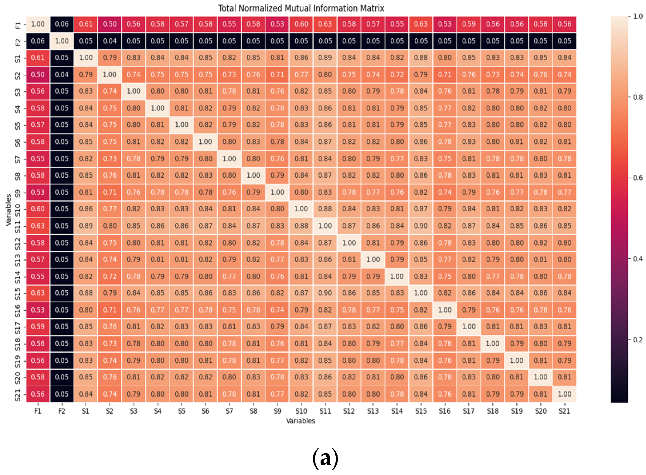
5.1. Results of Spatial Modelling

The object of spatial modelling is to incorporate the flow data of highly correlated stations into the model to improve the prediction accuracy. MI was used to measure the spatial correlation of stations using the flow data. The results of MI among all stations are shown in Figure 2. According to the results, the station XiaoZhai was selected as the correlated station of the predicted station, Zhonglou. The MI value was 0.9, which is higher than other stations.

5.2. Results of Time Interval Determination

When predicting metro flow, data with different historical time intervals can lead to different results. Shorter time intervals might not provide enough input data for the model to capture time-related patterns, while longer intervals could incorporate irrelevant inputs. Thus, to determine the optimal number of historical time intervals for superior predictive performance, this study incorporates historical data with different time intervals into the model to forecast entry and exit flows for the next time interval. The entry and exit metro flow prediction results of different historical time intervals for the two selected stations are illustrated in Table 2.
The results indicate that the optimal historical time intervals for predicting entry and exit flow at Zhonglou Station are 48 and 56, respectively. Similarly, the optimal historical time intervals for predicting entry and exit flow at Hangtiancheng Station are 52 and 58, respectively. Taking Zhonglou Station’s entry flow prediction as an example, when the input time interval was set to 48, the RMSE, MAE, and MAPE were 71.27, 46.85, and 10.35%, respectively. Notably, the MAPE exhibited the most significant decrease compared to other time intervals. The model demonstrated the best predictive performance under these specific input time intervals. Therefore, this time interval configuration was adopted for subsequent experiments.

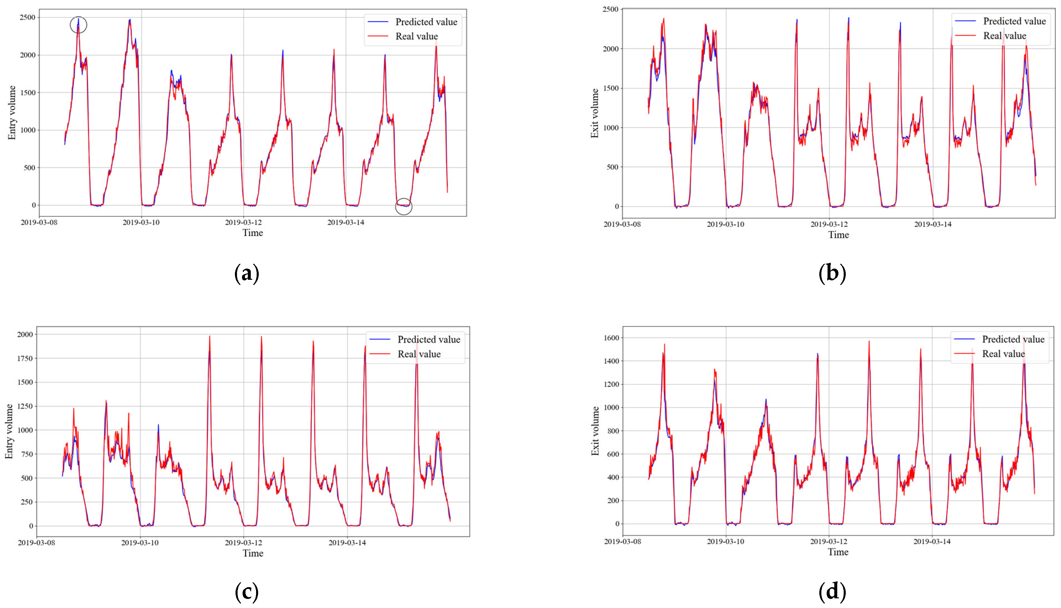
5.3. The Predicted Results of the Selected Stations

Table 3 presents the specific numerical values of three evaluation indicators for entry and exit metro flow predictions at Zhonglou Station and Hangtiancheng Station using different methods. In comparison to baseline methods (LSTM, GRU, transformer), the proposed method based on the transformer (MFP-EP) framework outperformed the baseline methods. The self-attention mechanism effectively captured the underlying long-term dependencies among features. Based on the results, incorporating various related data can improve the prediction accuracy. The model considers the influence of the upstream flow, the correlated stations, the recent historical metro flow, the historical temporal trend, and the external factors.
Moreover, when incorporating all factors comprehensively, the predictive accuracy was higher compared to considering individual factors separately. For instance, taking Zhonglou Station’s entry flow as an example, the overall predictive performance of MFP-EP + F1 + F2 + 2S + 4C was the best among the methods considered. Its RMSE, MAE, and MAPE values were 68.60, 45.86, and 10.04%, respectively. Compared to the transformer method, these values decreased by 13.58%, 18.56%, and 64.50%, respectively. Additionally, when compared to LSTM, these values decreased by 18.18%, 20.37%, and 67.08%, respectively.

5.4. Analysis of Prediction Results

Figure 3 illustrates the distribution of predicted values versus actual values when the model comprehensively considered factors such as temperature, precipitation, and the actual metro flow of the two stations that were most correlated to the target station based on the transformer method. According to the figure, it is evident that the distribution of predicted values closely aligns with the actual values, with most predictions closely matching the real data. The model successfully captured the peak and off-peak patterns of entry and exit flow. In Figure 3a, the peaks and troughs are marked with hollow circles. The peak occurred during the evening rush hours, specifically between 17:00 and 19:00, while the trough corresponds to the early morning hours when the subway services are temporarily halted.
Furthermore, the experimental results indicate that the peak entry and exit flows at Zhonglou Station are generally higher than those at Hangtiancheng Station. Both stations exhibited certain patterns, with variations in entry and exit flow between weekdays and weekends. Specifically, the peak entry and exit flows at Zhonglou Station typically ranged between 2000 and 2500, whereas at Hangtiancheng Station, the peak flow usually ranged between 1400 and 2000. This study then explained the flow changes from the perspective of urban functional zones. POI data within an 800 m radius around Zhonglou Station and Hangtiancheng Station were collected, as shown in Table 4. The data in the table refers to the number of POIs of a specific type within 800 m of the site. For example, 884 refers to the number of food and beverage services within 800 m of Zhonglou Station. The results indicate significantly higher numbers for sports and leisure services, accommodation services, public facilities, and scenic spots around Zhonglou Station (256, 900, 91, 35, respectively) compared to Hangtiancheng Station (53, 166, 10, 7, respectively). This suggests that Zhonglou Station serves as a commercial and tourist hub with a relatively high population density. Additionally, the number of companies, government institutions, and social organizations around Zhonglou Station is notably higher than around Hangtiancheng Station, indicating a larger daily population flow.
Moreover, 10 March 2019 was a Sunday, a typical rest day for most people. As expected, the entry and exit flows at the target stations significantly decreased on this day. In contrast, from 11 March to 15 March, which fall within the workweek, the entry and exit flows exhibit similar patterns. Additionally, the residential areas around Hangtiancheng Station are noticeably more abundant than around Zhonglou Station. This indicates that Hangtiancheng Station is located in a residential area, resulting in lower entry and exit counts on weekends compared to weekdays. In contrast, Zhonglou Station, as a tourist destination, experiences higher entry and exit counts on weekends compared to weekdays.
Finally, a few predicted values deviated from the actual values, which could be attributed to prediction errors caused by uncertain events. This observation aligns with the real urban traffic conditions, where traffic congestion during peak hours and unexpected traffic incidents can irregularly impact travel demand data, thus reducing the model’s predictive accuracy.

5.5. Analysis of Time Interval Correlation by Attention Mechanism

In comparison to other time intervals, the network focuses more on learning the entry flow of nearby time intervals within the same day. Taking the prediction of entry flow at Zhonglou Station as an example, Figure 4 illustrates the attention weight distribution obtained from an attention layer with a time interval of 48 steps. The horizontal axis represents the time steps, with each tick indicating one time interval, and the color intensity indicates the corresponding attention weight. For instance, consider Figure 4a, where the prediction time is 8:45~9:00. Time steps 2, 46, 47, and 48, corresponding to the time intervals 9:00~9:15, 20:00~20:15, 20:15~20:30, and 20:30~20:45, respectively, have relatively higher attention weights. These time intervals represent specific periods on the same day, as well as on previous days and weeks. Furthermore, Zhonglou Station is located near popular tourist attractions, and the entry flow during these time intervals remains high throughout the day, as the predicted time interval also falls within the peak period.

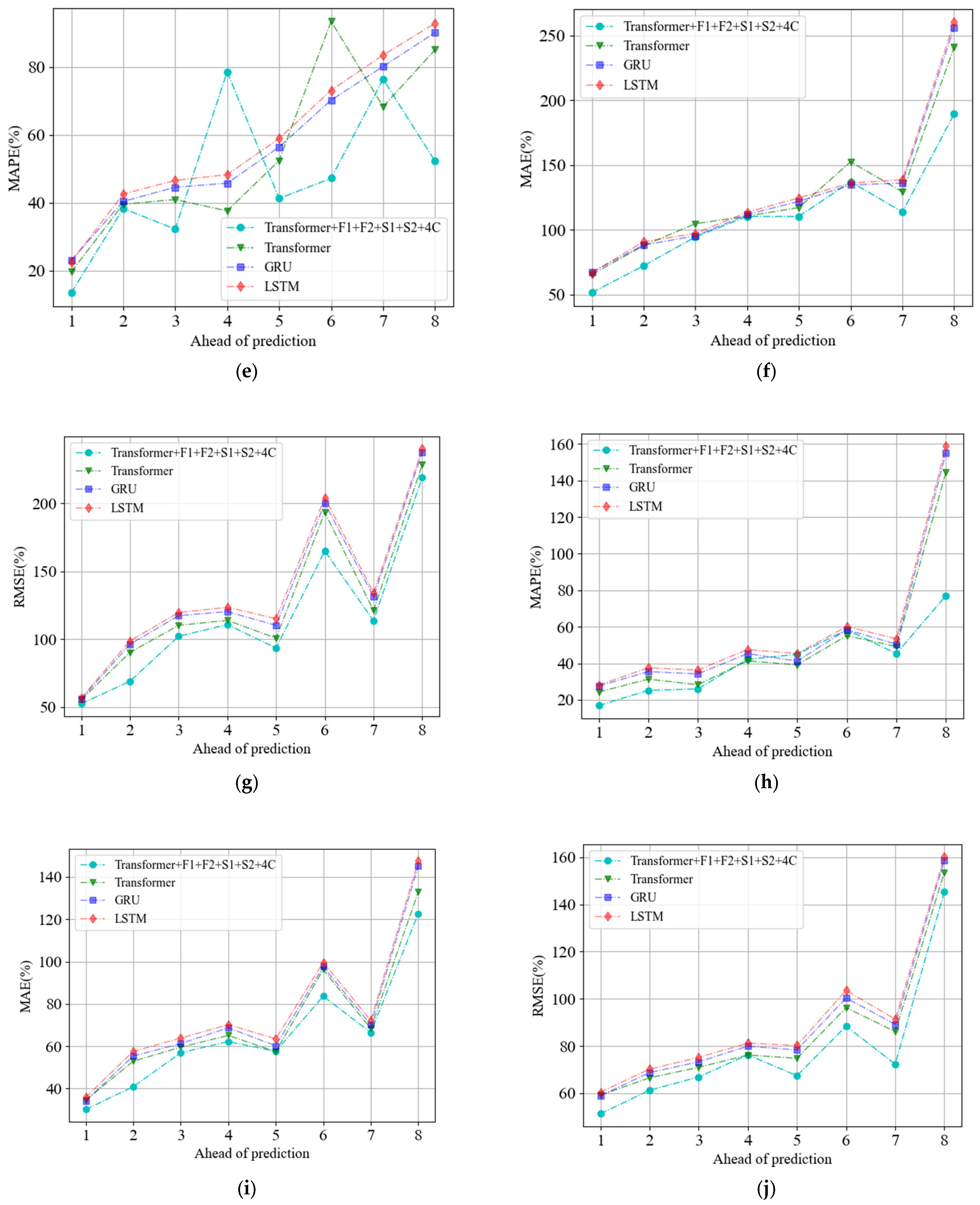
5.6. Analysis of Multi-Step Prediction Results for Entry and Exit Flow

The predictive performance of the model was also validated for multi-step metro flow prediction. Figure 5 illustrates the multi-step prediction results for the next eight steps (2 h). Compared with the baseline method, the proposed method is more accurate over a longer prediction period. Specifically, compared with the LSTM model, the mean values of MFP-EP + F1 + F2 + S1 + S2 for RMSE, MAE, and MAPE were reduced by 15%, 24.63%, and 34.02%, respectively, when the predicted step size is 2, and the proposed method was reduced by 6.5%, 7.26%, and 34.70%, respectively, compared with the mean of the baseline method when the predicted step size was 8.
The prediction error increased with the prediction step size. There are two main reasons for this. Firstly, compared with single-step prediction, the error accumulates in the process of multi-step prediction. The larger the number of prediction steps, the greater the accumulated error. Secondly, with the increase in time steps, the traffic environment gradually becomes complex, and the nonlinearity and fluctuation of the flow data in and out of the station gradually increase.
Compared with deep learning methods such as LSTM, the performance advantage of the proposed method in multi-step prediction is more obvious. This is not only due to the fact that the self-attention mechanism of the transformer model can capture more information in the time series prediction, but also because the model considers the temperature, the precipitation, the flow of the correlated stations, and the flow of different time granularities. The error accumulation rate of the method in multi-step prediction is much lower than that of methods such as LSTM.

6. Conclusions and Future Works

In conclusion, this study emphasizes the importance of integrating spatiotemporal and semantic aspects in metro flow prediction. To accurately predict metro flow, a novel deep learning model is proposed considering the spatial correlations, the temporal correlations from different time granularity, and the external weather factors. To model the spatial correlations, mutual information is leveraged to explore the nonlinear flow patterns between stations and determine the highly correlated stations. Then, the metro flow of recent historical time intervals, the metro flow at the same time intervals of previous days and weeks, and the temperature and precipitation data are combined and incorporated as the input data. Then, the multi-source and multi-dimensional data are fed into the transformer neural network. The self-attention mechanism of the network allows for effective handling of multidimensional data and enhances the accuracy of long-term predictions by focusing on key features. Extensive experiments with real data from the Xi’an subway validate our method’s efficacy, providing insights into significant features and moments that impact metro flow. Additionally, with POI information around the selected stations, our study delves into the fluctuations in metro flow. This analysis has the potential to offer valuable insights and practical recommendations for management authorities. The proposed method and comprehensive analysis highlight the significant potential of our approach in enhancing the accuracy and applicability of metro flow predictions in urban settings.
In the future, we will explore how to incorporate the distribution of POI features into the prediction model, investigating the influence of POI size and the distribution of geographical location on entry and exit traffic flow. Additionally, we will collect data on sudden events to study their impact on passenger flow and develop prediction models accordingly.

Author Contributions

Conceptualization, B.S. and Q.Y.; methodology, B.S. and Z.W.; formal analysis, Q.Y. and N.Y.; resources, J.Y.; data curation, Z.W.; writing—original draft preparation, B.S., Z.W. and J.Y.; writing—review and editing, B.S. and N.Y.; supervision, Q.Y. All authors have read and agreed to the published version of the manuscript.

Funding

This research was supported by the Fundamental Research Funds for the Central Universities, CHD (No. 300102210521).

Institutional Review Board Statement

Not applicable.

Informed Consent Statement

Not applicable.

Data Availability Statement

The data presented in this study are available on request from the corresponding author. The data are not publicly available due to the data are part of an ongoing study.

Conflicts of Interest

The authors declare no conflict of interest.

References

  1. Sperry, B.R.; Dye, T. Impact of new passenger rail stations on ridership demand and passenger characteristics: Hiawatha service case study. Case Stud. Transp. Policy 2020, 8, 1158–1169. [Google Scholar] [CrossRef]
  2. Yuan, C.; Feng, J.; Chen, J. Multi-step Passenger Demand Prediction Based on Spatiotemporal Correlation Incorporating Semantic Information. China J. Highw. Transp. 2023, 36, 207–219. [Google Scholar]
  3. Zhang, N.; Chen, F.; Zhu, Y.D.; Peng, H.; Wang, J.P.; Li, Y. A Study on the Calculation of Platform Sizes of Urban Rail Hub Stations Based on Passenger Behavior Characteristics. Math. Probl. Eng. 2020, 2020, 3689760. [Google Scholar] [CrossRef]
  4. da Silva, C.B.P.; Saldiva, P.H.N.; Amato-Lourenço, L.F.; Rodrigues-Silva, F.; Miraglia, S.G.E. Evaluation of the air quality benefits of the subway system in Sao Paulo, Brazil. J. Environ. Manag. 2012, 101, 191–196. [Google Scholar] [CrossRef] [PubMed]
  5. Liu, J.; Meng, B.; Wang, J.; Chen, S.Y.; Tian, B.; Zhi, G.Q. Exploring the Spatiotemporal Patterns of Residents’ Daily Activities Using Text-Based Social Media Data: A Case Study of Beijing, China. ISPRS Int. J. Geo-Inf. 2021, 10, 389. [Google Scholar] [CrossRef]
  6. Liu, L.; Chen, R.-C.; Zhu, S. Impacts of Weather on Short-Term Metro Passenger Flow Forecasting Using a Deep LSTM Neural Network. Appl. Sci. 2020, 10, 2962. [Google Scholar] [CrossRef]
  7. Li, L.C.; Wang, Y.G.; Zhong, G.; Zhang, J.; Ran, B. Short-to-medium Term Passenger Flow Forecasting for Metro Stations using a Hybrid Model. KSCE J. Civ. Eng. 2018, 22, 1937–1945. [Google Scholar] [CrossRef]
  8. Wang, X.M.; Zhang, N.; Zhang, Y.L.; Shi, Z.B. Forecasting of Short-Term Metro Ridership with Support Vector Machine Online Model. J. Adv. Transp. 2018, 2018, 3189238. [Google Scholar] [CrossRef]
  9. Tang, L.; Zhao, Y.; Cabrera, J.; Ma, J.; Tsui, K.L. Forecasting Short-Term Passenger Flow: An Empirical Study on Shenzhen Metro. IEEE Trans. Intell. Transp. Syst. 2019, 20, 3613–3622. [Google Scholar] [CrossRef]
  10. Ling, H.; Xu, H. A Study on the Factors Influencing the Passenger throughput of Civil Aviation in Sichuan Province Based on Multi-linear Regression Model. In Proceedings of the 2023 6th International Conference on Artificial Intelligence and Big Data (ICAIBD), Chengdu, China, 26–29 May 2023; pp. 11–15. [Google Scholar]
  11. Li, W.; Zhou, M.; Dong, H. CPT Model-Based Prediction of the Temporal and Spatial Distributions of Passenger Flow for Urban Rail Transit under Emergency Conditions. J. Adv. Transp. 2020, 2020, 8850541. [Google Scholar] [CrossRef]
  12. Liu, S.; Yao, E. Holiday Passenger Flow Forecasting Based on the Modified Least-Square Support Vector Machine for the Metro System. J. Transp. Eng. Part A Syst. 2017, 143, 04016005. [Google Scholar] [CrossRef]
  13. Hou, Z.; Du, Z.; Yang, G.; Yang, Z. Short-Term Passenger Flow Prediction of Urban Rail Transit Based on a Combined Deep Learning Model. Appl. Sci. 2022, 12, 7597. [Google Scholar] [CrossRef]
  14. Jing, Y.; Hu, H.; Guo, S.; Wang, X.; Chen, F. Short-Term Prediction of Urban Rail Transit Passenger Flow in External Passenger Transport Hub Based on LSTM-LGB-DRS. IEEE Trans. Intell. Transp. Syst. 2021, 22, 4611–4621. [Google Scholar] [CrossRef]
  15. Mo, B.C.; Zhao, Z.; Koutsopoulos, H.N.; Zhao, J.H. Individual Mobility Prediction in Mass Transit Systems Using Smart Card Data: An Interpretable Activity-Based Hidden Markov Approach. IEEE Trans. Intell. Transp. Syst. 2022, 23, 12014–12026. [Google Scholar] [CrossRef]
  16. Wang, Y.; Zheng, D.; Luo, S.M.; Zhan, D.M.; Nie, P. The Research of Railway Passenger Flow Prediction Model Based on BP Neural Network. Adv. Mater. Res. 2013, 605, 2366–2369. [Google Scholar] [CrossRef]
  17. Liu, L.; Wu, M.; Chen, R.-C.; Zhu, S.; Wang, Y. A Hybrid Deep Learning Model for Multi-Station Classification and Passenger Flow Prediction. Appl. Sci. 2023, 13, 2899. [Google Scholar] [CrossRef]
  18. Xiong, Z.; Zheng, J.; Song, D.; Zhong, S.; Huang, Q. Passenger Flow Prediction of Urban Rail Transit Based on Deep Learning Methods. Smart Cities 2019, 2, 371–387. [Google Scholar] [CrossRef]
  19. Liu, Y.; Liu, Z.; Jia, R. DeepPF: A deep learning based architecture for metro passenger flow prediction. Transp. Res. Part C Emerg. Technol. 2019, 101, 18–34. [Google Scholar] [CrossRef]
  20. Ouyang, Q.; Lv, Y.; Ma, J.; Li, J. An LSTM-Based Method Considering History and Real-Time Data for Passenger Flow Prediction. Appl. Sci. 2020, 10, 3788. [Google Scholar] [CrossRef]
  21. Shi, G.F.; Luo, L.M. Prediction and Impact Analysis of Passenger Flow in Urban Rail Transit in the Postpandemic Era. J. Adv. Transp. 2023, 2023, 3448864. [Google Scholar] [CrossRef]
  22. Mei, Z.Y.; Yu, W.T.; Tang, W.; Yu, J.H.; Cai, Z.Y. Attention mechanism-based model for short-term bus traffic passenger volume prediction. IET Intell. Transp. Syst. 2023, 17, 767–779. [Google Scholar] [CrossRef]
  23. Wang, K.; Guo, B.; Yang, H.; Li, M.; Zhang, F.; Wang, P. A semi-supervised co-training model for predicting passenger flow change in expanding subways. Expert Syst. Appl. 2022, 209, 118310. [Google Scholar] [CrossRef]
  24. Zeng, J.; Tang, J. Combining knowledge graph into metro passenger flow prediction: A split-attention relational graph convolutional network. Expert Syst. Appl. 2023, 213, 118790. [Google Scholar] [CrossRef]
  25. Xie, P.; Ma, M.; Li, T.; Ji, S.; Du, S.; Yu, Z.; Zhang, J. Spatio-Temporal Dynamic Graph Relation Learning for Urban Metro Flow Prediction. IEEE Trans. Knowl. Data Eng. 2023, 35, 9973–9984. [Google Scholar] [CrossRef]
  26. Yang, Y.J.; Zhang, J.L.; Yang, L.X.; Yang, Y.; Li, X.H.; Gao, Z.Y. Short-term passenger flow prediction for multi-traffic modes: A Transformer and residual network based multi-task learning method. Inf. Sci. 2023, 642, 119144. [Google Scholar] [CrossRef]
  27. Xu, Y.H.; Lyu, Y.; Xiong, G.W.; Wang, S.Y.; Wu, W.W.; Cui, H.L.; Luo, J.Z. Adaptive Feature Fusion Networks for Origin-Destination Passenger Flow Prediction in Metro Systems. IEEE Trans. Intell. Transp. Syst. 2023, 24, 5296–5312. [Google Scholar] [CrossRef]
  28. Jia, H.W.; Luo, H.Y.; Wang, H.; Zhao, F.; Ke, Q.X.; Wu, M.Y.; Zhao, Y.N. ADST: Forecasting Metro Flow Using Attention-Based Deep Spatial-Temporal Networks with Multi-Task Learning. Sensors 2020, 20, 4574. [Google Scholar] [CrossRef]
  29. Li, P.K.; Ma, C.Q.; Ning, J.; Wang, Y.; Zhu, C.H. Analysis of Prediction Accuracy under the Selection of Optimum Time Granularity in Different Metro Stations. Sustainability 2019, 11, 5281. [Google Scholar] [CrossRef]
  30. Koesdwiady, A.; Soua, R.; Karray, F. Improving Traffic Flow Prediction With Weather Information in Connected Cars: A Deep Learning Approach. IEEE Trans. Veh. Technol. 2016, 65, 9508–9517. [Google Scholar] [CrossRef]
  31. Zhang, J.L.; Chen, F.; Cui, Z.Y.; Guo, Y.A.; Zhu, Y.D. Deep Learning Architecture for Short-Term Passenger Flow Forecasting in Urban Rail Transit. IEEE Trans. Intell. Transp. Syst. 2021, 22, 7004–7014. [Google Scholar] [CrossRef]
  32. Zhang, J.B.; Zheng, Y.; Qi, D.K. Deep Spatio-Temporal Residual Networks for Citywide Crowd Flows Prediction. In Proceedings of the Thirty-First Aaai Conference on Artificial Intelligence, San Francisco, CA, USA, 4–9 February 2017; pp. 1655–1661. [Google Scholar]
  33. Chen, E.H.; Ye, Z.R.; Wang, C.; Xu, M.T. Subway Passenger Flow Prediction for Special Events Using Smart Card Data. IEEE Trans. Intell. Transp. Syst. 2020, 21, 1109–1120. [Google Scholar] [CrossRef]
  34. Wei, Y.; Chen, M.-C. Forecasting the short-term metro passenger flow with empirical mode decomposition and neural networks. Transp. Res. Part C Emerg. Technol. 2012, 21, 148–162. [Google Scholar] [CrossRef]
  35. Jia, Y.; He, P.; Liu, S.; Cao, L. A Combined Forecasting Model for Passenger Flow Based on GM and ARMA. Int. J. Hybrid Inf. Technol. 2016, 9, 215–226. [Google Scholar] [CrossRef]
  36. Lee, S.; Fambro, D.; Lee, S.; Fambro, D. Application of Subset Autoregressive Integrated Moving Average Model for Short-Term Freeway Traffic Volume Forecasting. Transp. Res. Rec. J. Transp. Res. Board 1999, 1678, 179–188. [Google Scholar] [CrossRef]
  37. Yan, D.; Zhou, J.; Zhao, Y.; Wu, B. Short-Term Subway Passenger Flow Prediction Based on ARIMA; Springer: Berlin/Heidelberg, Germany, 2018; pp. 464–479. [Google Scholar]
  38. Yao, K.; Gao, G.; Liu, Y.; Ju, X.; Zhang, Z. A Stable Passenger Flow Forecast Approach for Newly Opened Metro Stations Based on Multi-Source Data and Random Forest Regression Model. In Proceedings of the 2022 3rd International Conference on Intelligent Design (ICID), Xi’an, China, 21–23 October 2022; pp. 249–254. [Google Scholar]
  39. Liu, L.J.; Chen, R.C. A novel passenger flow prediction model using deep learning methods. Transp. Res. Part C-Emerg. Technol. 2017, 84, 74–91. [Google Scholar] [CrossRef]
  40. Shen, C.Z.; Zhu, L.; Hua, G.F.; Zhou, L.Y.; Zhang, L. A Deep Convolutional Neural Network Based Metro Passenger Flow Forecasting System Using a Fusion of Time and Space. In Proceedings of the 2020 IEEE 23RD International Conference on Intelligent Transportation Systems (ITSC), Rhodes, Greece, 20–21 September 2020. [Google Scholar]
  41. Sun, Y.Q.; Liao, K.L. A hybrid model for metro passengers flow prediction. Syst. Sci. Control Eng. 2023, 11, 2191632. [Google Scholar] [CrossRef]
  42. Zhang, X.R.; Wang, C.; Chen, J.W.; Chen, D. A deep neural network model with GCN and 3D convolutional network for short-term metro passenger flow forecasting. IET Intell. Transp. Syst. 2023, 17, 1559–1607. [Google Scholar] [CrossRef]
Figure 1. The research framework of this study.
Applsci 14 01949 g001
Figure 2. Total normalized mutual information matrix. (a) Mutual information calculated by entry flow. (b) Mutual information calculated by exit flow.
Applsci 14 01949 g002aApplsci 14 01949 g002b
Figure 3. Entry and exit volume of Zhonglou Station and Hangtiancheng Station. (a) Entry volume prediction results for Zhonglou Station. (b) Exit volume prediction results for Zhonglou Station. (c) Entry volume prediction results for Hangtiancheng Station. (d) Exit volume prediction results for Hangtiancheng Station.
Applsci 14 01949 g003
Figure 4. Attention matrices generated by the transformer framework. (a) Time interval: 8:45–9:00. (b) Time interval: 6:45–9:00.
Applsci 14 01949 g004aApplsci 14 01949 g004b
Figure 5. Results of multi-step metro flow prediction using different methods. (a) MAPE of entry of Zhonglou station. (b) RMSE of entry of Zhonglou station. (c) MAE of entry of Zhonglou station. (d) RMSE of exit of Zhonglou station. (e) MAPE of exit of Zhonglou station. (f) MAE of exit of Zhonglou station. (g) RMSE of entry of Hangtiancheng station. (h) MAPE of entry of Hangtiancheng station. (i) MAE of entry of Hangtiancheng station. (j) RMSE of exit of Hangtiancheng station. (k) MAPE of exit of Hangtiancheng station. (l) MAE of exit of Hangtiancheng station.
Applsci 14 01949 g005aApplsci 14 01949 g005bApplsci 14 01949 g005c
Table 1. Subway station descriptions.
Station NumberStation Name
S1Beikezhan Station
S2Beiyuan Station
S3Yundonggongyuan Station
S4Xingzhengzhongxin Station
S5Fengchengwulu Station
S6Shitushuguan Station
S7Daminggongxi Station
S8Longshouyuan Station
S9Anyuanmen Station
S10Beidajie Station
S11Zhonglou Station
S12Yongningmen Station
S13Nanshaomen Station
S14Tiyuchang Station
S15Xiaozhai Station
S16Weiyijie Station
S17Huizhanzhongxin Station
S18Sanyao Station
S19Fengqiyuan Station
S20Hangtiancheng Station
S21Weiqunan Station
Table 2. The entry and exit flow prediction results of different historical time intervals.
Time IntervalEvaluating Indicators
Zhonglou Station (Entry)Zhonglou Station (Exit)Hangtiancheng Station (Entry)Hangtiancheng Station (Exit)
RMSEMAEMAPERMSEMAEMAPERMSEMAEMAPERMSEMAEMAPE
2475.2549.3213.69%91.0861.4222.71%56.3136.3025.37%61.1540.4639.58%
2878.2051.7613.67%91.9959.5123.55%56.1034.7516.37%60.5941.2444.43%
3274.9048.5420.52%88.7757.4120.76%56.1234.0416.54%58.6739.0542.97%
3678.7350.2117.14%88.6760.0314.85%56.1534.8218.25%59.8239.5535.64%
4074.5148.8217.14%90.4163.1435.93%55.9837.8331.40%54.3937.2331.49%
4473.1049.2219.02%88.4560.9520.05%54.2933.4620.82%54.6236.9736.77%
4871.2746.8510.35%85.7859.5026.49%53.4633.5119.12%52.8035.1918.78%
5269.2745.3416.02%87.2459.5715.40%53.8332.3517.89%54.0136.0430.34%
5670.5547.8919.14%86.2855.5213.97%55.0133.0517.83%53.6936.2727.52%
6067.6345.3014.75%93.8660.8418.00%54.7433.4019.63%53.6036.6535.14%
Table 3. Prediction results for the selected stations.
Experimental MethodsZhonglou Station (Entry)Zhonglou Station (Exit)Hangtiancheng Station (Entry)Hangtiancheng Station (Exit)
RMSEMAEMAPERMSEMAEMAPERMSEMAEMAPERMSEMAEMAPE
LSTM83.8457.5930.50%96.7266.9422.52%56.5735.8328.06%60.3938.6836.50%
GRU82.6655.0031.24%96.6667.3522.99%55.8434.2127.52%58.9140.3838.74%
Transformer79.3856.3128.28%96.9065.4919.56%55.2134.5024.24%59.1540.8033.25%
MFP-EP + F172.5748.0615.24%92.2564.9643.82%55.7334.6118.04%54.7838.9141.23%
MFP-EP + F272.8648.2216.44%97.2963.1815.53%53.8835.2121.55%55.5737.8231.28%
MFP-EP + F1 + F270.4347.6819.33%90.7761.1523.06%55.1235.1427.73%54.5338.0138.24%
MFP-EP + 1S72.5849.5520.13%93.6160.9323.32%54.8533.3921.71%54.3537.0125.89%
MFP-EP + 2S70.0648.0810.80%83.5655.7318.71%53.3136.4721.83%55.0637.4235.20%
MFP-EP + F1 + F2 + 2S71.2746.8510.35%86.2855.5213.97%53.8332.3517.89%52.8035.1918.78%
MFP-EP + F1 + F2 + 2S + 4C68.6045.8610.04%80.2651.5213.35%52.4230.2416.83%51.3933.8317.84%
Table 4. POI data within an 800 m radius around Zhonglou Station and Hangtiancheng Station.
POIZhonglou StationHangtiancheng Station
Food and beverage services884792
Shopping services838882
Life services888811
Sports and leisure services25653
Health care services160188
Accommodation services900166
Scenic spots357
Government agencies and social organizations216115
Science and education cultural services149114
Transportation facilities services26369
Financial and insurance services8139
Incorporated businesses30281
Public facilities9110
Industrial parks02
Residential areas71105
Disclaimer/Publisher’s Note: The statements, opinions and data contained in all publications are solely those of the individual author(s) and contributor(s) and not of MDPI and/or the editor(s). MDPI and/or the editor(s) disclaim responsibility for any injury to people or property resulting from any ideas, methods, instructions or products referred to in the content.

