Abstract
The present state of research in computational fluid dynamics (CFD) is marked by an ongoing process of refining numerical methods and algorithms with the goal of achieving accurate modeling and analysis of fluid flow and heat transfer phenomena. Remarkable progress has been achieved in the domains of turbulence modeling, parallel computing, and mesh generation, resulting in heightened simulation precision when it comes to capturing complex flow behaviors. Nevertheless, CFD faces a significant challenge due to the time and expertise needed for a meticulous simulation setup and intricate numerical techniques. To surmount this challenge, we introduce paint2sim—an innovative mobile application designed to enable on-the-fly 2D fluid simulations using a device’s camera. Seamlessly integrated with OpenLB, a high-performance Lattice Boltzmann-based library, paint2sim offers accurate simulations. The application leverages the capabilities of the Lattice Boltzmann Method (LBM) to model fluid behaviors accurately. Through a symbiotic interaction with the open-source OpenCV library, paint2sim can scan and extract hand-drawn simulation domains, affording the capability for instant simulation and visualization. Notably, paint2sim can also be regarded as a digital twin, facilitating just-in-time representation and analysis of 2D fluid systems. The implications of this technology extend significantly to both fluid dynamics education and industrial applications, effectively lowering barriers and rendering fluid simulations more accessible. Encouragingly, the outcomes of simulations conducted with paint2sim showcase promising qualitative and quantitative results. Overall, paint2sim offers a groundbreaking approach to mobile 2D fluid simulations, providing users with just-in-time visualization and accurate results, while simultaneously serving as a digital twin for fluid systems.
1. Introduction
Computational fluid dynamics (CFD) has been a vital tool for understanding fluid behavior across various industries and academic domains. However, the practical application of CFD has been limited by the long computational time and complexity involved in building a simulation setup. In recent years, the integration of CFD into various software, including CAD, 3D computational graphic software like Blender version 4.0.2 [1], and game engines like Unity version 2023.2.10 [2] and Unreal Engine version 5.3 [3], has become more prevalent due to its usefulness in observing fluid flow behavior.
Various researchers have proposed innovative methods for applying CFD to different areas of interest. Mathias Berger and Verina Cristie [4] proposed using game engine technology to bridge the gap between architects and engineers in evaluating the effect of buildings on urban climate through CFD methods. Jos Stam [5] presented a rapid implementation of a fluid dynamics solver for game engines based on the physical equations of fluid flow, emphasizing stability and speed for just-in-time performance. Wangda Zuo and Qingyan Chen [6] proposed the Fast Fluid Dynamics (FFD) method as an intermediate approach between nodal models and CFD, providing much richer flow information while being 50 times faster than CFD for conducting faster-than-just-in-time flow simulations for emergency management in buildings. Angela Minichiello et al. [7] introduced a mobile instructional particle image velocimetry (mI-PIV) tool for smartphones and tablets running Android that provides guided instruction to learners, enabling them to visualize and experiment with authentic flow fields in real time. Jia-Rui et al. [8] explore the use of augmented reality (AR) technology in mobile devices for visualizing and interacting with CFD simulation results in the context of indoor thermal environment design. Harwood et al. [9] developed a GPU-accelerated, interactive simulation framework suitable for mobile devices, enabling the visualization of flow around particles.
The Lattice Boltzmann Method (LBM), a versatile computational technique for simulating fluid flow, is integral to our approach. Renowned for its capability to handle intricate geometries, multiple phases, and mesoscale phenomena [10], the LBM operates on a lattice grid, utilizing probability distribution functions to model fluid behavior, and it is adaptable for parallel processing on diverse platforms. Recent advancements include the integration of multiple-relaxation-time schemes to enhance stability and efficiency, along with extensions for simulating thermal and multiphase flows [11,12]. The LBM finds application in various scenarios, such as solving evaporating and boiling problems [13], observing particle behavior in particle-laden flows [14], simulating heat transfer [15], and more.
Previously mentioned work [9] utilized a static domain with fixed inlets and outlets to create 2D simulations on tablets, which is limited to NVIDIA GPU-based devices.
In this paper, we present a new application called paint2sim version 0.1, which extends the capabilities of OpenVisFlow version 0.1 [16], a visualization library that introduced novel solutions to the challenges of a long computational time and complexity when targeting mobile devices. Leveraging the power of the LBM, paint2sim utilizes the open-source library OpenCV version 4.8.1 [17] to enable on-the-fly, just-in-time 2D simulations using the camera of a mobile device. Our approach is not limited to specific NVIDIA GPU-based mobile devices but is applicable to all Android devices. Furthermore, we incorporate AR capabilities through the scanning of physical objects. Moreover, in this paper, we compare the performance, demonstrating better results even while utilizing only one core.
The aim of this approach is to enable users to generate a digital twin of a fluid domain using hand-drawn sketches, effectively converting their mobile devices into virtual laboratories for fluid dynamics. The objective is to facilitate the scanning of a simulation domain and provide real-time visualization of calculated results just in time, eliminating the need for precompiled simulations or specialized expertise. By seamlessly connecting physical sketches with real-time simulations, paint2sim strives to function as a digital twin for 2D fluid flow simulations.
Our contributions include the integration of the Lattice Boltzmann-based library OpenLB version 1.5 [18] into the mobile device, just-in-time simulation and visualization, as well as stable simulations for most cases. The application paint2sim plays a pivotal role in advancing applied CFD by providing students and engineers with a user-friendly platform for quick insights into 2D fluid dynamics. The unique feature of generating just-in-time simulations on mobile devices empowers users to swiftly visualize and analyze fluid behavior in real-time, enhancing the accessibility and efficiency of fluid flow studies.
This technology has the potential to revolutionize how we teach and learn fluid dynamics, as well as how we design and optimize fluid-based systems. paint2sim has the potential to benefit a wide range of users and applications, from students learning the fundamentals of fluid dynamics to engineers designing complex systems in the chemical, aerospace, and automotive industries. The technology can also be applied in medical research and environmental studies, where fluid behavior plays a crucial role. By simplifying the simulation process and making it more accessible, paint2sim has the potential to democratize the field of CFD and encourage a wider range of users to explore the fascinating world of fluid dynamics.
In the remainder of this paper, we delve into the method employed by paint2sim, present the numerical results obtained through its implementation, and engage in a comprehensive discussion of these results. A user guide with a download link for paint2sim can be found in Appendix A.
2. Method
There are three critical requirements that must be fulfilled in order to run scanned hand-drawn simulation domains and simulate them locally on mobile devices: a high performance to simulate and visualize the simulation just in time, a high stability due to the various domains that can be scanned and the adjustable Reynolds number, and the physical accuracy should have quantitatively minimal errors and should be qualitatively comparable to reality.
In the following sections, we discuss the LBM, the simulation model used in this study, and its suitability for a high performance and physical accuracy. Following that, we describe the methods utilized to ensure the stability of the simulation.
2.1. Lattice Boltzmann Method (LBM)
The LBM offers several advantages when it comes to both performance and physical accuracy in simulating fluid behavior. One advantage is that the LBM can be easily parallelized, allowing for faster computation times and higher performance. Another advantage is that the LBM inherently models the fluid at a mesoscopic level, allowing for an accurate representation of complex physical phenomena such as turbulence and multiphase flows. This makes the LBM well-suited for simulating a wide range of fluid dynamics problems. In the remainder of this section, we provide a brief introduction to the LBM and the target equations, the Navier–Stokes Equations (NSE) for mass and momentum conservation in fluid dynamics.
The NSE is the fundamental equation that governs the behavior of fluids, and it is widely used in CFD simulations. The NSE in full form can be solved only numerically using various discretization methods, such as the finite difference, finite volume method or the LBM.
The NSE can be written as follows:
where is the velocity vector, p is the pressure, is the fluid density, is the molecular kinematic viscosity of the fluid, and is the external force acting on the fluid.
The LBM approximates the conservation equations in its limit (Chapman–Enskog expansion) on a discrete grid of points connected by a set of links that represent the paths along which the fluid particles can move [19]. In the LBM, the spatial and temporal states of these particles are represented by the probability distribution functions (PDFs) that evolve according to the lattice Boltzmann equation.
where is the PDF at lattice node i and time t, is the normalized discrete velocity in the i-th direction, is the collision operator, and is the Guo forcing term [20].
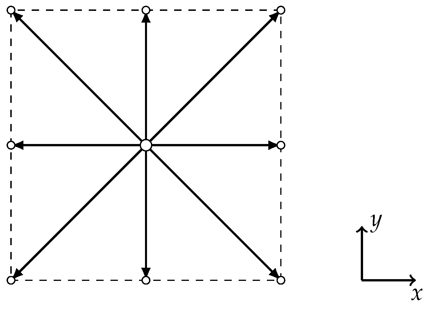
In the current simulations, the D2Q9 lattice is used, where D is the number of dimensions and Q is the number of the normalized discrete velocity directions. The corresponding lattice cell is shown in Figure 1.

Figure 1.
A schematic illustration of the discrete velocity set for the lattice.
2.2. Smagorinsky BGK Collision Model
The Smagorinsky model [21] is a subgrid-scale model used in a large eddy simulation (LES) of turbulent flows. The model introduces a turbulent viscosity term to the governing equations of fluid flow, which is based on the strain rate tensor of the flow field. The model filters out the small unresolved vortices by replacing them with an artificial viscosity increase. The large eddies are preserved. The modified strain rate tensor describes the production of turbulent kinetic energy in the flow.
The turbulent viscosity term is given by the following:
where is the turbulent eddy viscosity, is the grid spacing, is the Smagorinsky constant, and is the magnitude of the strain rate tensor. The Smagorinsky constant is the filtering parameter that determines which eddies are neglected.
The modified momentum equation with the addition of the turbulent viscosity term becomes the following:
For the incompressible NSE with a Smagorinsky LES approach, the lattice Boltzmann equation using the BGK collision operator [22] can be rewritten as follows:
where is the effective relaxation time adapted to the Smagorinsky model. Here, is the discrete speed of sound.
Due to obstacles in the path of a fluid, flow instabilities can be induced even at low Reynolds numbers. Therefore, it is necessary to adjust the relaxation time accordingly. The Smagorinsky BGK model accomplishes this by automatically increasing the relaxation time at the cells with a high shear rate. In the case of a laminar flow, the turbulent viscosity . Choosing a correct Smagorinsky constant secures a stable run of the simulation.
2.3. Fringe Region Technique
A fringe region technique [23] is used to eliminate instabilities at the outflow boundary condition. The outlet can become divergent if a large eddy flows through it. In order to compensate for this, a fringe zone is applied to laminarize the outflow. To achieve this, the NSE in the near-to-outlet region is forced with a special term.
where is the prescribed velocity, is the fringe function that varies smoothly from 0 to 1 over a distance of a few grid points, and is the computed velocity.
In the fringe region technique, the prescribed velocity is obtained using a mixing length model. The mixing length model can be written as follows:
where is the velocity at a point x, is the outlet coordinate, and are tuning parameters for transition between real and prescribed velocities, and S is a smooth function that varies from 0 to 1 over a distance.
2.4. Concept and Realization
The implementation of the system used two separate shared libraries: one for OpenCV and one for OpenLB. OpenCV provided the image processing capabilities, while OpenLB provided the CFD simulation capabilities. The shared libraries were written in C++ and can be compiled on a variety of platforms. The implementation involved creating a set of functions that could be used by both the OpenCV and OpenLB libraries. These functions were used to perform image processing and CFD simulation, respectively. In addition, Unity was used to create the application for the mobile device. Both OpenCV and OpenLB communicate independently with Unity through their respective shared libraries.
2.4.1. Concept
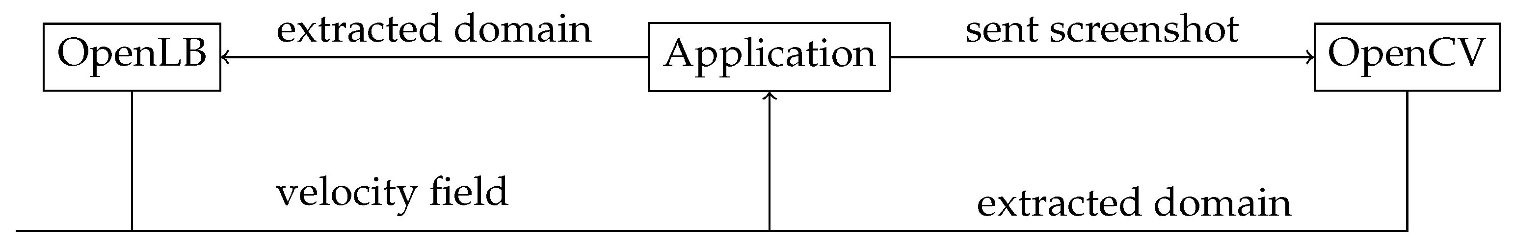
In order to achieve just-in-time simulation and visualization, there must be a clear separation between the frontend, which is the application itself, and the backend, which consists of the OpenLB and OpenCV shared libraries. Each of the shared libraries is called in separate threads which allows for the decoupling of the simulation and visualization thereof. The communication between the frontend and backend consists primarily of the exchange of the simulation results for a timestep in the form of a pressure or velocity array as shown in Figure 2.
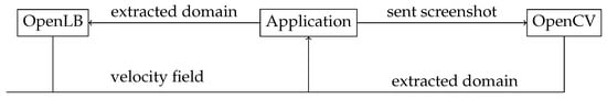
Figure 2.
Communication between the application, OpenCV, and OpenLB.
2.4.2. Structure of the OpenLB Shared Library
In this section, we present an overview of the OpenLB shared library structure that we employed for performing the simulations on smartphones. Specifically, Algorithm 1 illustrates the main loop of the library, which adheres to the standard Lattice Boltzmann simulation structure with OpenLB. Initially, OpenLB is instantiated, and crucial classes are initialized. The unit converter, which stores the lattice relevant data, is then declared. Next, the simulation domain is instantiated, and its dimensions correspond to the domain scanned with the smartphone. This domain is then passed to the load balancer, which distributes the cuboid into subsections necessary for parallel computing. The material number map is an array of numbers that refer to the materials in the simulation. However, it cannot be utilized as is and necessitates a transfer to the OpenLB-specific class, superGeometry. After preparing the geometry, the lattice is ready for simulation, and boundary conditions can be set. In particular, we apply the Smagorinksy BGK model in Section 2.2 to the material numbers of the fluid outflow and inflow. Additionally, we utilize the fringe region technique around the outflow. Moreover, we need to specify which material numbers define the inlet and outlet. We also add the postprocessor, which receives relevant dimensions and pointers to the result arrays. At step 10 of Algorithm 1, the simulation commences with the for-loop. In this loop, T corresponds to the total simulation time, while iT represents the current timestep. For each timestep, we update and set the boundary values. Subsequently, we call the collide and stream functions to retrieve the values for the subsequent step. Finally, we synchronize the number of timesteps saved per second with the frames per second () of the smartphone application (step 13 to 21). This synchronization ensures better performance as we do not save every timestep of the simulation but still maintain a fluid visualization for the user.
| Algorithm 1 Mainloop of the OpenLB Shared Library | |
| 1: | init OpenLB |
| 2: | declare unit converter |
| 3: | instantiation of the simulation domain |
| 4: | instantiation of a load balancer |
| 5: | preparing of the geometry |
| 6: | preparing of the lattice |
| 7: | add postprocessor |
| 8: | calculate the number of timesteps from the total simulation time T |
| 9: | start timer |
| 10: | for ; ; do |
| 11: | set boundary values |
| 12: | collide and stream |
| 13: | if then |
| 14: | if & then |
| 15: | write results via postprocessor |
| 16: | write Mega Lattice Updates per Second |
| 17: | end if |
| 18: | count++ |
| 19: | end if |
| 20: | reset |
| 21: | count = 0; |
| 22: | if endSimulation then break; |
| 23: | end if |
| 24: | end for |
2.4.3. Structure of the OpenCV Shared Library
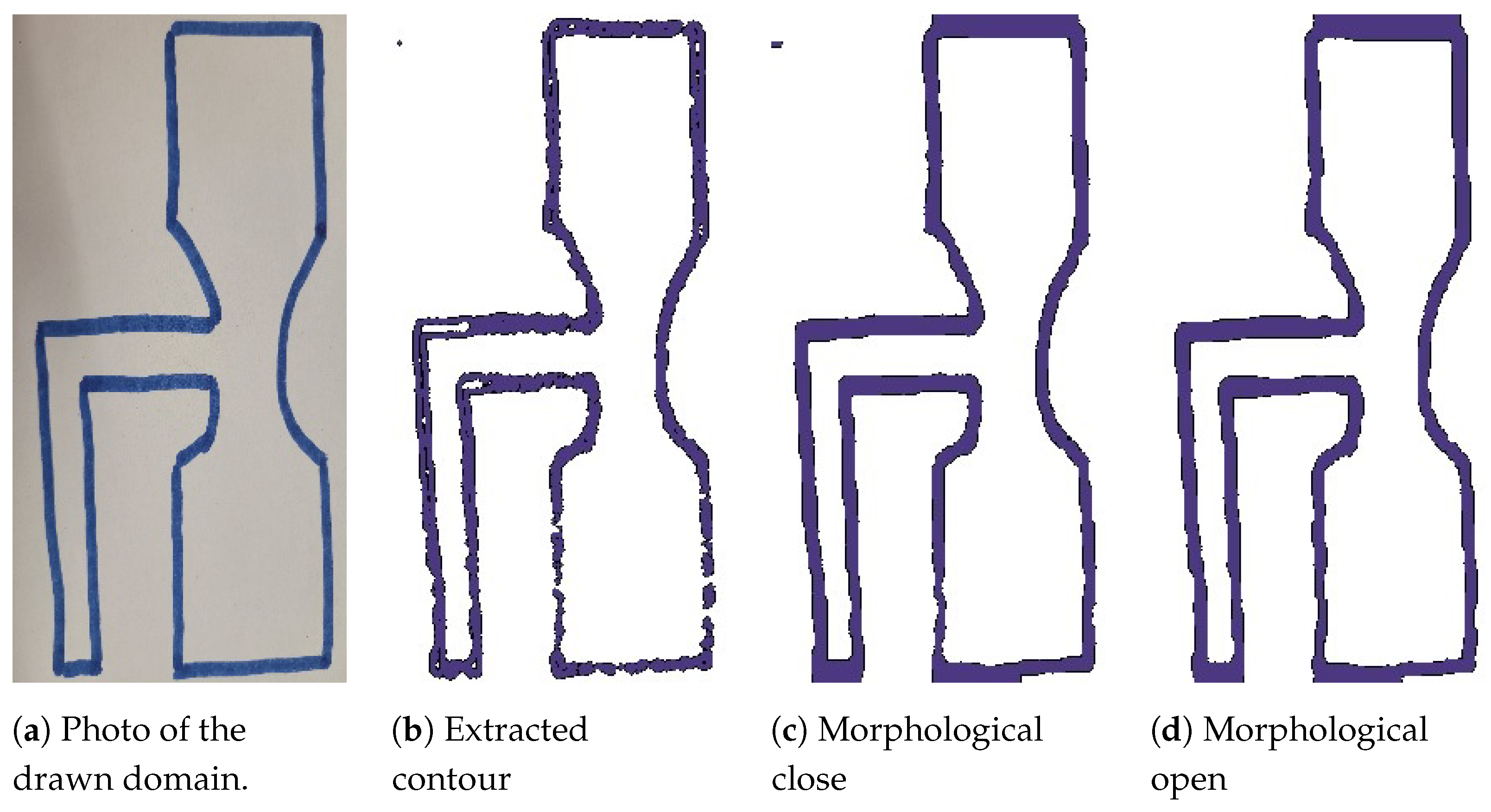
The OpenCV shared library plays a critical role in enabling OpenVisFlow to extract contours, which is a vital step in obtaining the simulation domain from an image. Contour extraction involves identifying the object’s boundary in an image and approximating it with a curve. The curve consists of continuous points along the boundary with the same color or intensity. The process of domain extraction begins by resizing the image to the desired simulation resolution, followed by applying a threshold to enhance the contrast between the domain and the background. The findContours function is then utilized to extract the domain boundaries. Finally, morphological functions are applied to postprocessing of the extracted domain. Specifically, a morphological close function is used to fill potential holes in the boundary, while a morphological open function is used to eliminate noise from the domain. Figure 3 displays the results of the processing steps, where Figure 3a depicts the photo of the hand-drawn domain to be extracted, and Figure 3b presents the outcome of the initial extraction with a threshold; Figure 3c,d represent the post-image processing steps.
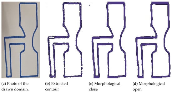
Figure 3.
The figure illustrates the domain extraction process, starting with the original image (a), followed by the resulting image after the initial extraction with a threshold (b). Post-image processing steps are then applied, leading to the final processed images shown in (c,d).
2.5. Expanding OpenVisFlow for Mobile Fluid Flow Simulation with OpenLB
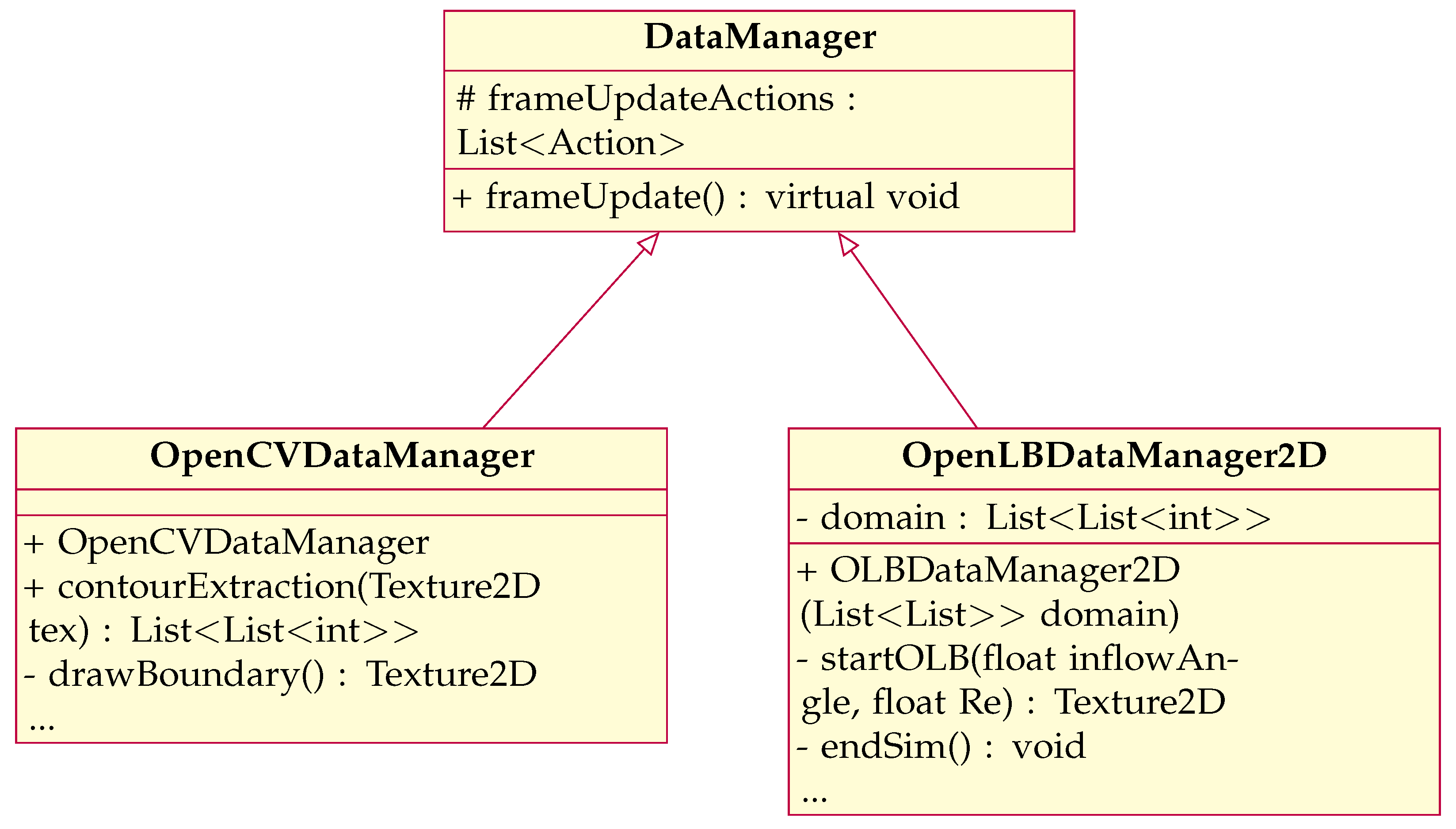
The OpenVisFlow library, based on Unity, is designed to be easily expandable, allowing it to handle and visualize various data types. To achieve this, two new classes are required that inherit from the parent DataManager class. These classes enable communication between OpenVisFlow and the shared libraries OpenLB and OpenCV. Figure 4 depicts the class diagram for the new classes, OpenCVDatamanger and OpenLBDatamanger, which inherit from the parent class Datamanager.
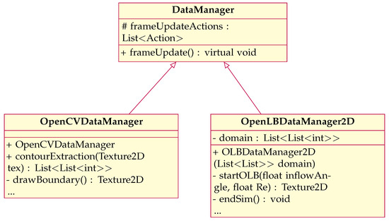
Figure 4.
Class diagram for the OpenCV and OpenLB DataManager, highlighting the most essential functions.
The OpenCVDataManager class adds necessary functions for communication between OpenVisFlow and the OpenCV shared library. Similarly, the OpenLBDataManager2D class inherits from DataManager and includes the essential functions required to initiate and terminate a simulation. The class also contains additional functionalities such as an optional placement of a fringe zone. Overall, these new classes ensure seamless communication between OpenVisFlow and the OpenLB and OpenCV shared libraries, allowing for efficient data handling and visualization.
Visualization of the Simulation Data
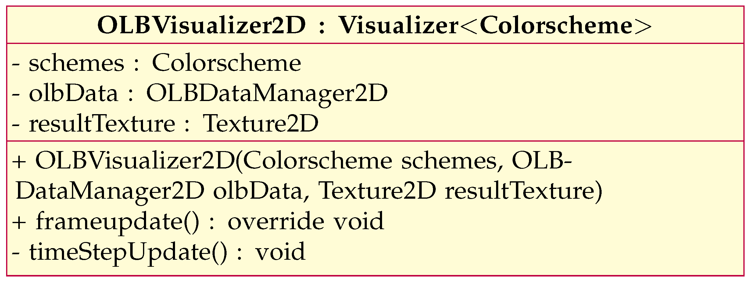
In order to visualize the calculated results of the OpenLB shared library introduced in Section 2.4.2, a new visualizer class has to be implemented which has the ability to handle 2D arrays of the type float, transform this information to a texture, and display it. The class diagram of the new class is depicted in Figure 5. Following the OpenVisFlow framework, the visualizer is initialized with a Colorscheme, which consist of different colors that are used to visualize the flow and an instance of the OLBDataManager2D in order to get the simulation data. The function timeStepUpdate is added to the inherited action list. This function is called on every frame and extracts the minimum and maximum bounds for the macroscopic moments of the current timestep. Based on that, the color scheme can be mapped to each cell and rendered to a texture for display.
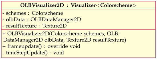
Figure 5.
Class diagram of the OLBVisualizer2D, highlighting the most essential functions.
3. Numerical Experiments and Discussion of Results
This section evaluates the precision and performance of the LBM as implemented in paint2sim. We categorize the results into qualitative and quantitative aspects. The qualitative section focuses on the visualization of the simulation results and their correspondence to physical reality. For the quantitative part, we assess the performance and physical accuracy of the simulation.
3.1. Test Case Setup
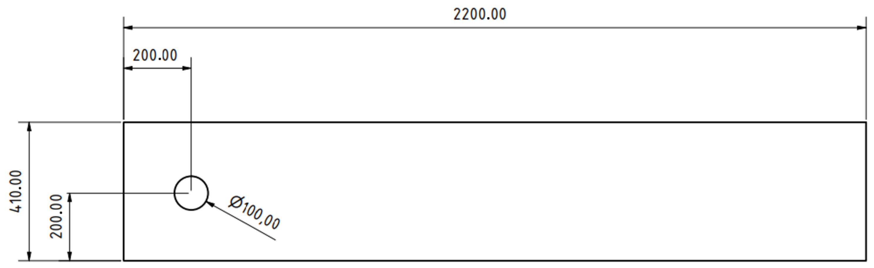
To validate the capabilities of paint2sim, we chose the 2D cylinder test case provided by the OpenLB library. This test case replicates the configuration detailed by Schäfer et al. [24]. This selection enables a direct comparison between the results generated by paint2sim and the established outcomes in the relevant domain. In addition, we recreated the same scenario through manual drawing, ensuring consistent proportions as outlined in the reference work [24]. Subsequently, the hand-drawn representation was scanned using paint2sim, enabling a precise evaluation of its accuracy in replicating the expected flow patterns and attributes. The geometry used for validation is visually presented in Figure 6.
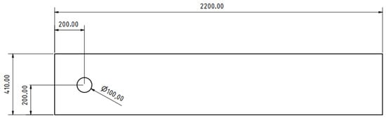
Figure 6.
Geometry employed for validation, with dimensions in SI millimeters.
It is important to note that, in this study, paint2sim incorporates the Smagorinsky BGK Model and the Fringe Region Technique to maintain simulation stability even at lower resolutions. Notably, the validated cylinder2D case does not utilize either of these techniques.
3.2. Choice of Discretization Parameters
To accommodate various performance capabilities on mobile devices, paint2Sim offers four resolution options in terms of , representing the voxel length. In alignment with this, we conducted corresponding simulations using the OpenLB framework. The timestep scales diffusively with the resolution, meaning that it decreases or increases quadratically in correspondence with . To demonstrate that OpenLB produces consistent results with those presented in Schäfer et al. [24], we also incorporated a higher resolution. Due to the performance restriction inherent in mobile devices, this higher resolution cannot be executed on mobile devices. paint2sim differs from the validation case in three aspects. Firstly, it employs the Smagorinsky BGK Collision Model. Secondly, it incorporates the fringe region technique to ensure stability. Thirdly, the application exclusively employs the Bounceback boundary condition instead of the Bouzidi second-order condition. The decision between the first and second orders is rooted in numerical analysis and depends on the nature of the boundary—being first order for curved boundaries and second order for axis-aligned cells. The prevalence of a first-order condition in most scenarios is attributed to the staircase approximation. This approach is preferred due to the challenging extraction of the real geometry surface required by Bouzidi from an already discretized scanned domain.
paint2sim-1: The fringe region technique as well as the Smagorinsky BGK Collision Model are used with the Smagorisnky Constant .
paint2sim-2: The fringe region technique is used while the Smagorinsky BGK Model is replaced with the BGK Collison Model.
paint2sim-3: The fringe region technique is removed, and the Smagorinsky BGK Model is replaced with the BGK Collison Model.
paint2sim-4: The fringe region technique is removed, and the Smagorinsky BGK Model is used.
In order to perform a comparison between Bouzidi and Bounceback, we also ran the validation case from OpenLB with Bouzidi OpenLB-1 and with Bounceback OpenLB-2.
3.3. Validation
3.3.1. Qualitative Results
Figure 7 presents a side-by-side comparison of the results. Observing the laminar flow at , there is no noticeable difference between the validated case shown in Figure 7a and the result obtained using paint2sim, as shown in Figure 7b. Furthermore, when comparing the unstable flow in Figure 7c,d, the qualitative results are also in agreement.
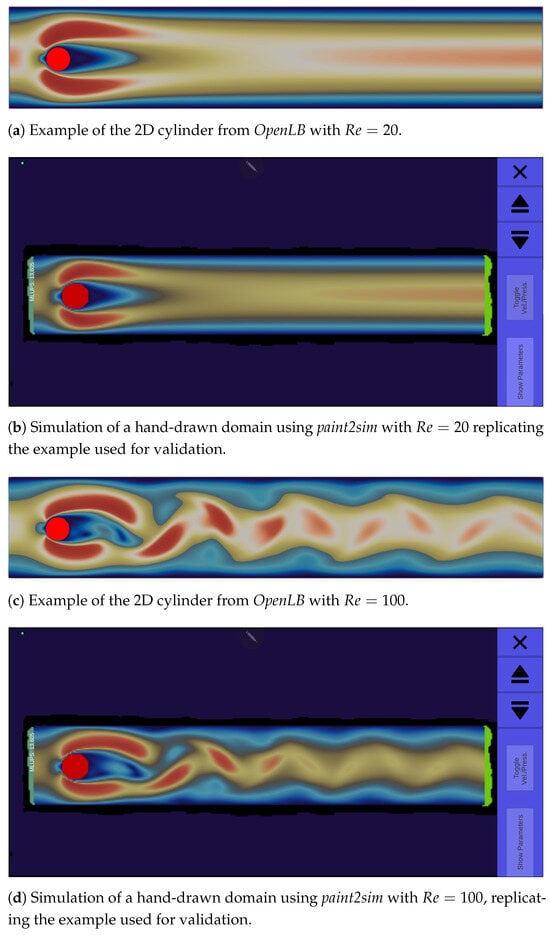
Figure 7.
Comparison of qualitative results for the flow around a cylinder between the OpenLB simulation cases validated by Schäfer et al. [24] and the paint2sim simulations.
3.3.2. Quantitative Results
This section presents a comparative assessment of the validation results obtained from [24], as depicted in Table 1, concerning the drag and lift coefficients on the cylinder, with both OpenLB and paint2sim. Table 2 presents the results of simulations conducted at , detailing the parameters and resulting drag and lift coefficients for specific cases. The results from OpenLB align within the predefined bounds set in Table 1 when utilizing a sufficiently high resolution. Conversely, paint2sim at its maximum resolution yields results that deviate by approximately 11% for the drag coefficient. Additionally, the lift coefficient exhibits considerable variation, failing to closely match the specified margin. This discrepancy primarily stems from errors introduced during the hand-drawn domain scan, where image processing techniques for domain extraction introduce slight shape differences, particularly in the representation of the cylinder within the domain. Given the current computational limitations of the mobile devices used for the scan and corresponding simulation resolution, addressing this issue comprehensively is presently impractical. Nevertheless, the results emphasize that an increase in resolution contributes to a reduction in the margin of error.

Table 1.
Results of drag and lift coefficients from Schäfer et al. [24] in a laminar flow around a cylinder with Re = 20 for the stable case and Re = 100 for the unstable case.
Table 2.
Comparative analysis of drag and lift coefficients: OpenLB vs. paint2sim in the flow around a cylinder at (stable case).
In Table 3, the outcomes for flow simulations at exhibit similar challenges to those encountered in the stable scenario at .
Table 3.
Comparative analysis of drag and lift coefficients: OpenLB vs. paint2sim in the flow around a cylinder at (unstable case).
3.4. Performance
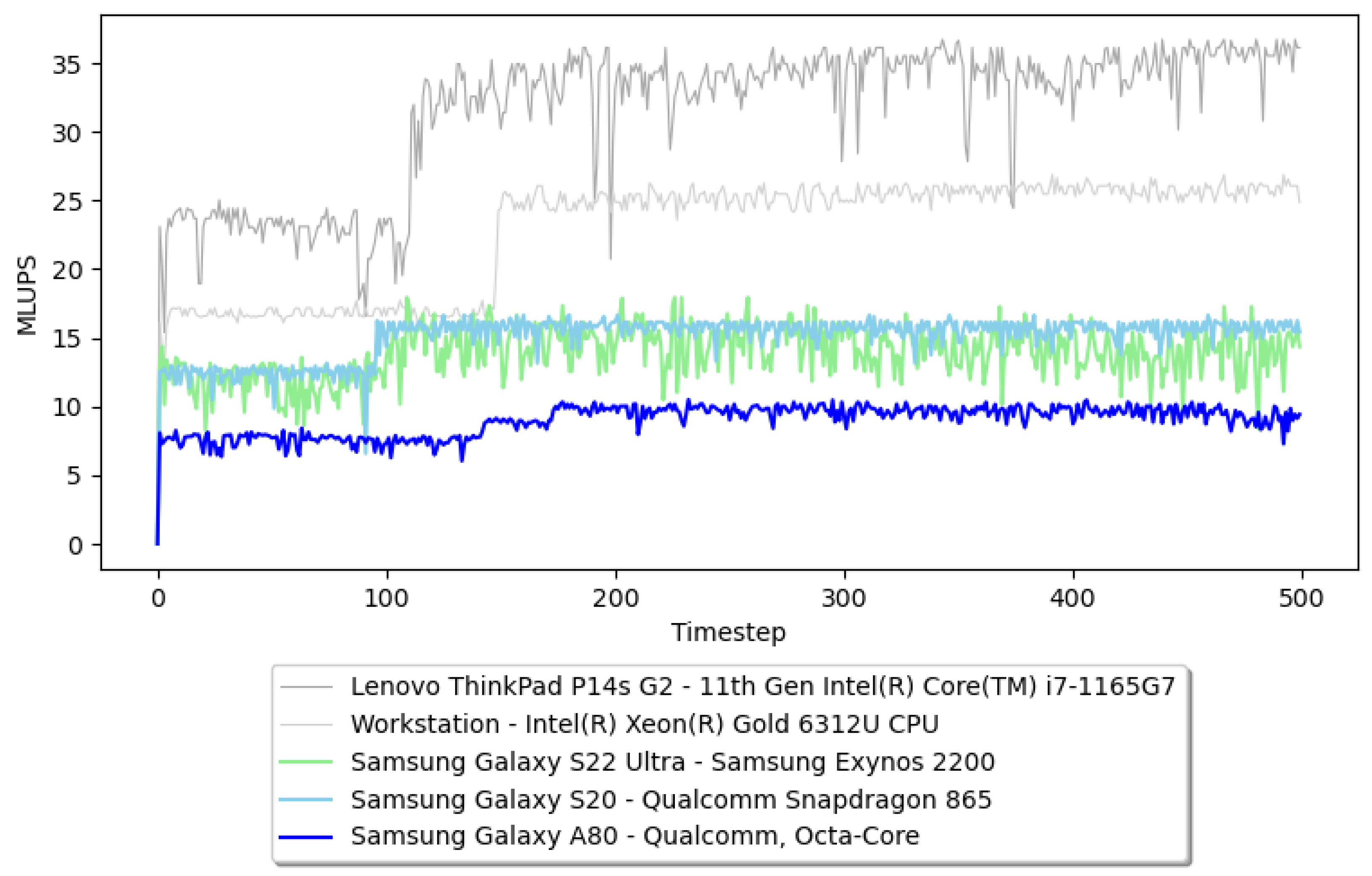
Figure 8 presents the total performance achieved by paint2sim measured in millions of cell updates per second (Mega Lattice Updates per Second (MLUPS)) across a set of mobile- and stationary test devices.
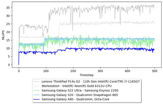
Figure 8.
Performance comparison of paint2sim across different devices. Performance is measured in Mega Lattice Updates per Second (MLUPS).
A central performance bottleneck for numerical simulations on mobile devices due to their inherent compute-heavy nature is given by heat management constraints. This is the primary explanation for visible performance fluctuations as mobile devices tend to aggressively reduce their power output beyond short performance bursts in order to prevent overheating.
While the underlying LBM library OpenLB supports various parallelization modes both on CPU and GPU targets [18,25], paint2sim explicitly only uses single-threaded, single-precision, non-vectorized execution for maximum device portability and as a heat-management trade-off. While OpenMP-based shared memory parallelization was possible, core heterogeneity and thread binding caused issues across the diverse set of test devices. Single-threaded execution provides sufficient cross-device performance for the intended two-dimensional flow simulations.
On the lowest end, we conducted a performance comparison between paint2sim and the results presented in [9]. Due to hardware availability issues, we were unable to use the same experimental setup and instead relied on a low-end Huawei P8 Lite with inferior specifications compared to the initial high-end NVIDIA Shield K1 Tablet. Table 4 presents a comparison of the specifications obtained via Geekbench, a well-established mobile benchmark suite, and the achieved total performance in MLUPS. Despite the decision to not utilize parallelization, paint2sim’s performance compares favourably at a speed-up of approximately .
Table 4.
Performance and spec comparison of Nvidia Shield Tablet K1 and Huawei P8 Lite. For the spec comparison and Single-Core Score Geekbench [26].
Among the tested mobile devices in Figure 8, the Samsung Galaxy A80 offers the lowest CPU performance. Despite this, the visualization remains smooth for users at an average throughput of 10 MLUPS and no noticeable lags. At the top end, the single-threaded LBM performance on a Samsung Galaxy S22 Ultra is quite close to the unvectorized performance on higher-end x86 CPU cores at approximately 24 MLUPs.
Overall, the performance characteristics exhibited by paint2sim are sufficient for the intended simulation cases and are highly competitive to single cores of full-powered x86 CPUs, considering the comparably smaller power envelope.
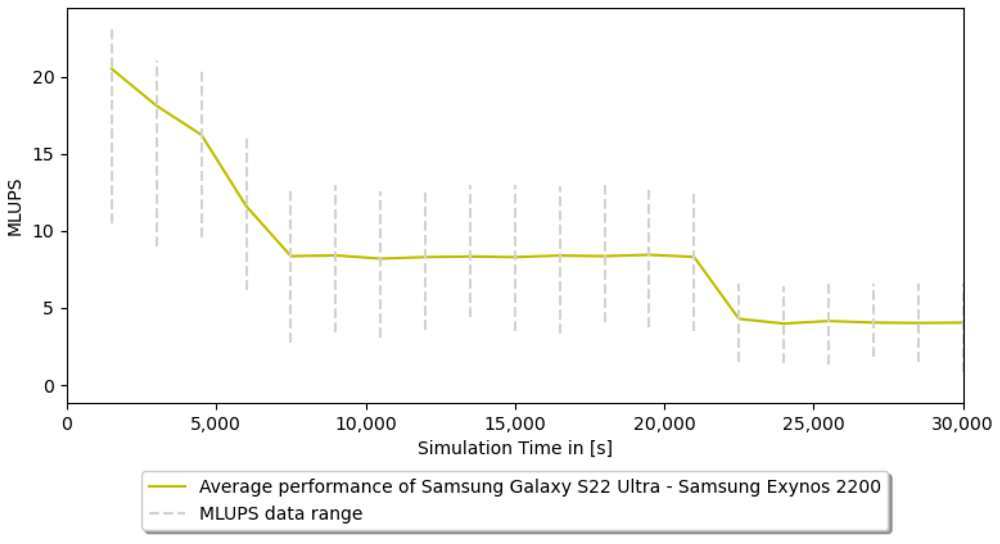
A notable issue associated with mobile devices is their tendency to decrease the power output of their CPUs in order to prevent overheating. Figure 9 presents the average MLPUs of the mobile device Samsung Galaxy S22 Ultra during extended simulation periods. The graph illustrates a significant decline in performance over time. Moreover, the decline is not continuous; rather, the device maintains its performance until the temperature reaches a critical point, at which it then ramps down to a lower performance level.
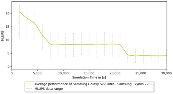
Figure 9.
Performance decline over time of paint2sim. Performance is measured in Mega Lattice Updates per Second (MLUPS).
3.5. Conclusions
In this paper, we present the paint2sim software for LBM simulations on mobile devices and the numerical validation of the software on an example of the Schäfer test case. The simulation results are categorized into qualitative and quantitative aspects, focusing on visualization, performance, and physical accuracy. Regarding performance, we analyzed the total performance achieved by paint2sim on various mobile devices. The Samsung Galaxy A80 exhibited the lowest CPU performance among the tested devices but still provided smooth visualization with an average of 10 Mega Lattice Updates per Second (MLUPS) and no noticeable lags. On the other hand, the Samsung Galaxy S22 Ultra demonstrated impressive performance, comparable to higher-end x86 CPUs, achieving the highest MLUPS of 24 under specific conditions. However, fluctuations in performance were observed due to heat management constraints, leading to an aggressive reduction in the CPU’s power output beyond short performance bursts.
The validation of paint2sim involved qualitative and quantitative comparisons. For the qualitative validation, we replicated a well-established 2D cylinder example using a hand-drawn image and compared the results with the validated case from OpenLB. The flow patterns and characteristics exhibited by paint2sim were found to be in agreement with the established findings. For the quantitative validation, we compared the drag and lift coefficients of the cylinder simulation with the results from previous studies: while the drag coefficients showed minor discrepancies of around ∼10%, the lift coefficients obtained from paint2sim differed greatly. These variations can be attributed to the shape approximation of the hand-drawn cylinder and slight inaccuracies in the scanned image.
Overall, the performance and accuracy of paint2sim on mobile devices proved to be sufficient for the intended simulation cases and to be highly competitive with full-powered x86 CPUs within a smaller power envelope. Further enhancements can be achieved through a parallelization of the application on mobile devices, which would significantly improve performance metrics. Future work should also address the issue of performance fluctuations resulting from heat management constraints. Taking these factors into account, the digital twin and virtual laboratory features of paint2sim hold the promise of offering a valuable simulation tool for 2D computational fluid dynamics applications, allowing for on-the-go simulations.
Author Contributions
Conceptualization, D.T.; methodology, D.T.; software, D.T.; validation, D.T.; formal analysis, D.T.; investigation, D.T.; resources, M.J.K.; data curation, D.T.; writing—original draft preparation, D.T.; writing—review and editing, A.K., F.B., M.D., and M.J.K.; supervision, M.J.K.; project administration, M.J.K.; funding acquisition, M.J.K. All authors have read and agreed to the published version of the manuscript.
Funding
This research was funded by The Ministry of Science, Research and the Arts of the State of Baden-Württemberg, grant number 34-7811.553-4/5, and by the Lattice Boltzmann Research Group.
Institutional Review Board Statement
Not applicable.
Informed Consent Statement
Not applicable.
Data Availability Statement
Data is contained within the article.
Conflicts of Interest
The authors declare no conflicts of interest.
Appendix A. User Guide for paint2sim
The application paint2sim is available for download at www.openlb.net/paint2sim/ (accessed on 18 February 2024). This section provides a detailed description of how to use the application. The forward/backward buttons are used to navigate between different steps, while the cross can be used to reset the application. All steps are shown in the remaining part of this section. It is advisable to use a thick fine-tip marker to draw the domain for an effective domain recognition.
Selecting Resolution: Begin by selecting your preferred resolution using the slider, as illustrated in Figure A1a. The options range from 100 to 300 in 50-unit increments, representing the number of cells across the screen width on your mobile device. Note that higher resolutions may impact user experience on certain devices, potentially causing performance issues.
Scanning the Domain: Utilize the scan button (Figure A1b) to initiate the domain-scanning process. Once completed, input the scale of the domain in meters (Figure A1c).
Setting Characteristic Length: Set the characteristic length for the Reynolds number estimation either through the input field or by adjusting the scale via touch (Figure A1d).
Edit the Domain: The domain can be edited using various touch-based options as shown in Figure A1e. The edit functions are as follows: Add walls; Remove existing walls; Declare particles for drag and lift calculations (currently limited to one particle); Define mandatory inlets and outlets.
Fluid Parameters: Choose fluid parameters from the dropdown menu, selecting Water, Oil, or Air. Alternatively, input custom kinematic viscosity and density values (Figure A1f).
Reynolds Number: Enter the Reynolds number for the simulation. (Figure A1h).
Inflow Direction: If not opting for a Poiseuille inflow, enter the desired inflow direction (Figure A1g).
Simulation: The final step initiates the simulation, which runs continuously until manually canceled using the back button or the cross button. During the simulation, toggle between velocity and pressure visualization methods, and view simulation parameters as needed.
If every step was performed correctly, the simulation should be running just in time on the mobile screen. In Figure A2, an example simulation is shown.

Figure A1.
The figures show the input menus of paint2sim to scan and set up a simulation.
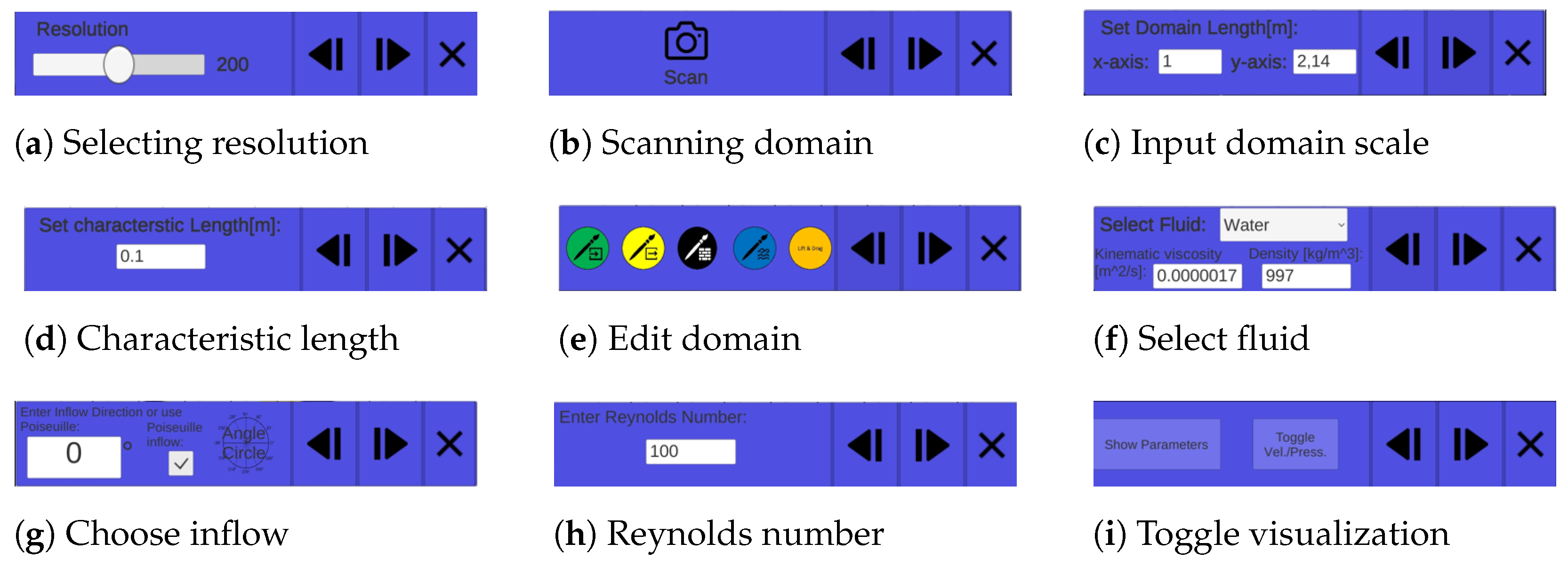
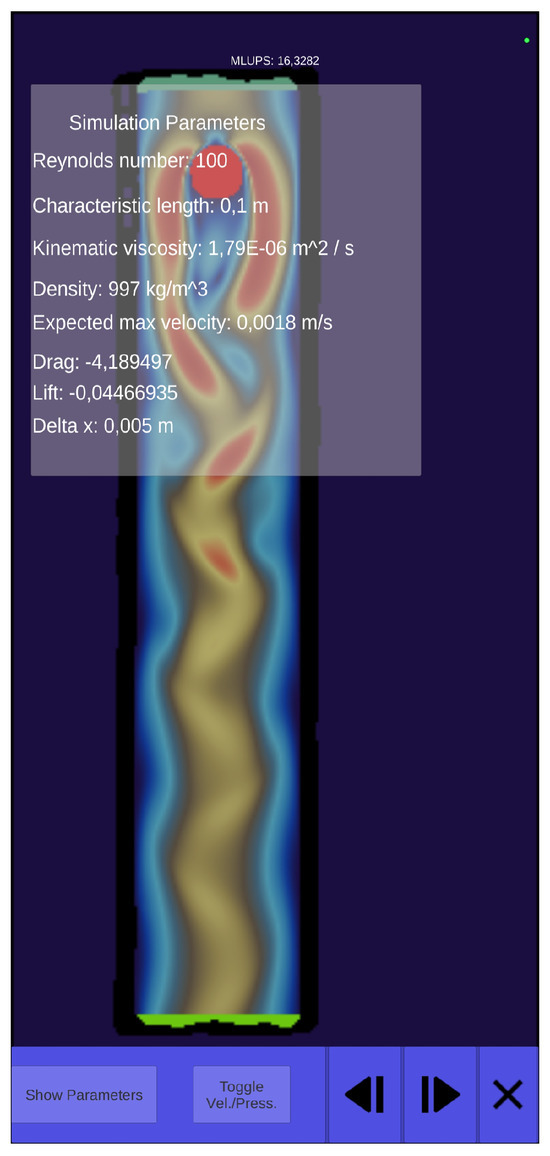
Figure A2.
Resulting example simulation after following each step (Figure A1a–i).

References
- Community, B.O. Blender—A 3D Modelling and Rendering Package; Blender Foundation, Stichting Blender Foundation: Amsterdam, The Netherlands, 2018. [Google Scholar]
- Unity Technologies Version 2023.2.10. San Francisco, CA, USA. Available online: https://unity.com (accessed on 2 February 2024).
- Epic Games. Unreal Engine Cary, NC, USA. Available online: https://www.unrealengine.com (accessed on 2 February 2024).
- Berger, M.; Cristie, V. CFD post-processing in Unity3D. Procedia Comput. Sci. 2015, 51, 2913–2922. [Google Scholar] [CrossRef]
- Stam, J. Real-time fluid dynamics for games. In Proceedings of the Game Developer Conference, San Jose, CA, USA, 4–8 March 2003; Volume 18, p. 25. [Google Scholar]
- Zuo, W.; Chen, Q. Real-time or faster-than-real-time simulation of airflow in buildings. Indoor Air 2009, 19, 33. [Google Scholar] [CrossRef] [PubMed]
- Minichiello, A.; Armijo, D.; Mukherjee, S.; Caldwell, L.; Kulyukin, V.; Truscott, T.; Elliott, J.; Bhouraskar, A. Developing a mobile application-based particle image velocimetry tool for enhanced teaching and learning in fluid mechanics: A design-based research approach. Comput. Appl. Eng. Educ. 2021, 29, 517–537. [Google Scholar] [CrossRef]
- Lin, J.R.; Cao, J.; Zhang, J.P.; van Treeck, C.; Frisch, J. Visualization of indoor thermal environment on mobile devices based on augmented reality and computational fluid dynamics. Autom. Constr. 2019, 103, 26–40. [Google Scholar] [CrossRef]
- Harwood, A.R.; Revell, A.J. Interactive flow simulation using Tegra-powered mobile devices. Adv. Eng. Softw. 2018, 115, 363–373. [Google Scholar] [CrossRef]
- Liu, Z.; Chu, X.; Lv, X.; Liu, H.; Fu, H.; Yang, G. Accelerating Large-Scale CFD Simulations with Lattice Boltzmann Method on a 40-Million-Core Sunway Supercomputer. In Proceedings of the 52nd International Conference on Parallel Processing, Salt Lake City, UT, USA, 7–10 August 2023; pp. 797–806. [Google Scholar] [CrossRef]
- Wenhan, Z.; Hong, F.; Gong, S. Improved multi-relaxation time thermal pseudo-potential lattice Boltzmann method with multi-block grid and complete unit conversion for liquid–vapor phase transition. Phys. Fluids 2023, 35, 053337. [Google Scholar] [CrossRef]
- Kuzmin, A.; Mohamad, A.; Succi, S. Multi-relaxation time Lattice Boltzmann Model for multiphase flows. Int. J. Mod. Phys. C 2008, 19, 875–902. [Google Scholar] [CrossRef]
- Li, Q.; Zhou, P.; Yan, H.J. Improved thermal lattice Boltzmann model for simulation of liquid-vapor phase change. Phys. Rev. E 2017, 96, 063303. [Google Scholar] [CrossRef] [PubMed]
- Dietzel, M.; Ernst, M.; Sommerfeld, M. Application of the Lattice-Boltzmann Method for Particle-laden Flows: Point-particles and Fully Resolved Particles. Flow Turbul. Combust. 2016, 97, 539–570. [Google Scholar] [CrossRef]
- Hamila, R.; Jemni, A.; Perre, P. A lattice Boltzmann source formulation for advection and anisotropic. Indian J. Phys. 2023, 97, 3047–3055. [Google Scholar] [CrossRef]
- Teutscher, D.; Weckerle, T.; Öz, F.; Krause, M.J. Interactive Scientific Visualization of Fluid Flow Simulation Data Using AR Technology-Open-Source Library OpenVisFlow. Multimodal Technol. Interact. 2022, 6, 81. [Google Scholar] [CrossRef]
- Bradski, G. The OpenCV Library. Dr. Dobb’s J. Softw. Tools 2000, 25, 120–123. [Google Scholar]
- Krause, M.J.; Kummerländer, A.; Avis, S.J.; Kusumaatmaja, H.; Dapelo, D.; Klemens, F.; Gaedtke, M.; Hafen, N.; Mink, A.; Trunk, R.; et al. OpenLB—Open source lattice Boltzmann code. Comput. Math. Appl. 2021, 81, 258–288. [Google Scholar] [CrossRef]
- Li, J. Appendix: Chapman-Enskog Expansion in the Lattice Boltzmann Method. arXiv 2015, arXiv:1512.02599. [Google Scholar] [CrossRef]
- Guo, Z.; Zheng, C.; Shi, B. Discrete lattice effects on the forcing term in the lattice Boltzmann method. Phys. Rev. E 2002, 65, 046308. [Google Scholar] [CrossRef] [PubMed]
- Smagorinsky, J. General Circulation Experiments with the Primitive Equations. Mon. Weather. Rev. 1963, 91, 99–164. [Google Scholar] [CrossRef]
- Bhatnagar, P.L.; Gross, E.P.; Krook, M. A Model for Collision Processes in Gases. I. Small Amplitude Processes in Charged and Neutral One-Component Systems. Phys. Rev. 1954, 94, 511–525. [Google Scholar] [CrossRef]
- Nordström, J.; Nordin, N.; Henningson, D. The fringe region technique and the Fourier method used in the direct numerical simulation of spatially evolving viscous flows. SIAM J. Sci. Comput. 1999, 20, 1365–1393. [Google Scholar] [CrossRef]
- Schäfer, M.; Turek, S.; Durst, F.; Krause, E.; Rannacher, R. Benchmark Computations of Laminar Flow around a Cylinder; Springer: Berlin/Heidelberg, Germany, 1996. [Google Scholar]
- Kummerländer, A.; Dorn, M.; Frank, M.; Krause, M.J. Implicit propagation of directly addressed grids in lattice Boltzmann methods. Concurr. Comput. Pract. Exp. 2023, 35, e7509. [Google Scholar] [CrossRef]
- Geekbench. Geekbench Browser. 2023. Available online: https://browser.geekbench.com/ (accessed on 22 June 2023).

Disclaimer/Publisher’s Note: The statements, opinions and data contained in all publications are solely those of the individual author(s) and contributor(s) and not of MDPI and/or the editor(s). MDPI and/or the editor(s) disclaim responsibility for any injury to people or property resulting from any ideas, methods, instructions or products referred to in the content. |
© 2024 by the authors. Licensee MDPI, Basel, Switzerland. This article is an open access article distributed under the terms and conditions of the Creative Commons Attribution (CC BY) license (https://creativecommons.org/licenses/by/4.0/).