

Underwater Degraded Image Restoration by Joint Evaluation and Polarization Partition Fusion

 ,
,
Abstract
1. Introduction
2. Underwater Degraded Image Restoration Methods
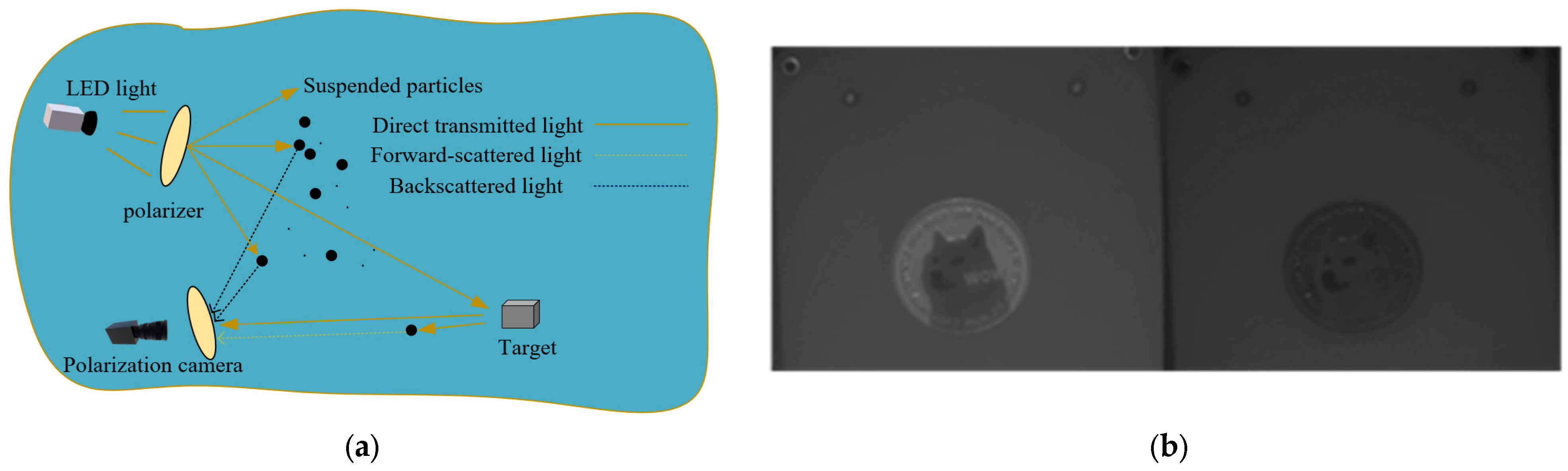
2.1. Underwater Polarization Image Restoration Model
2.2. Imin, Imax Pre-Processing
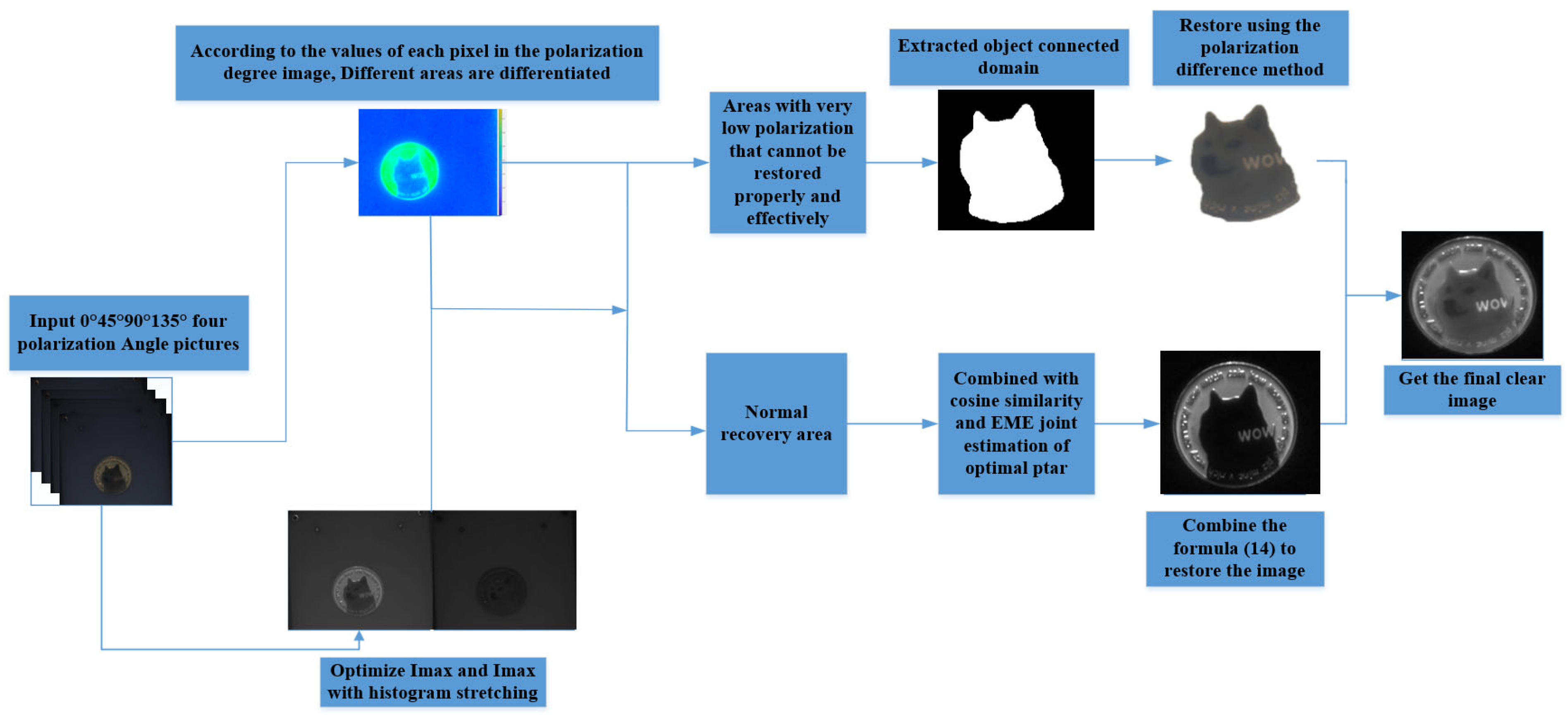
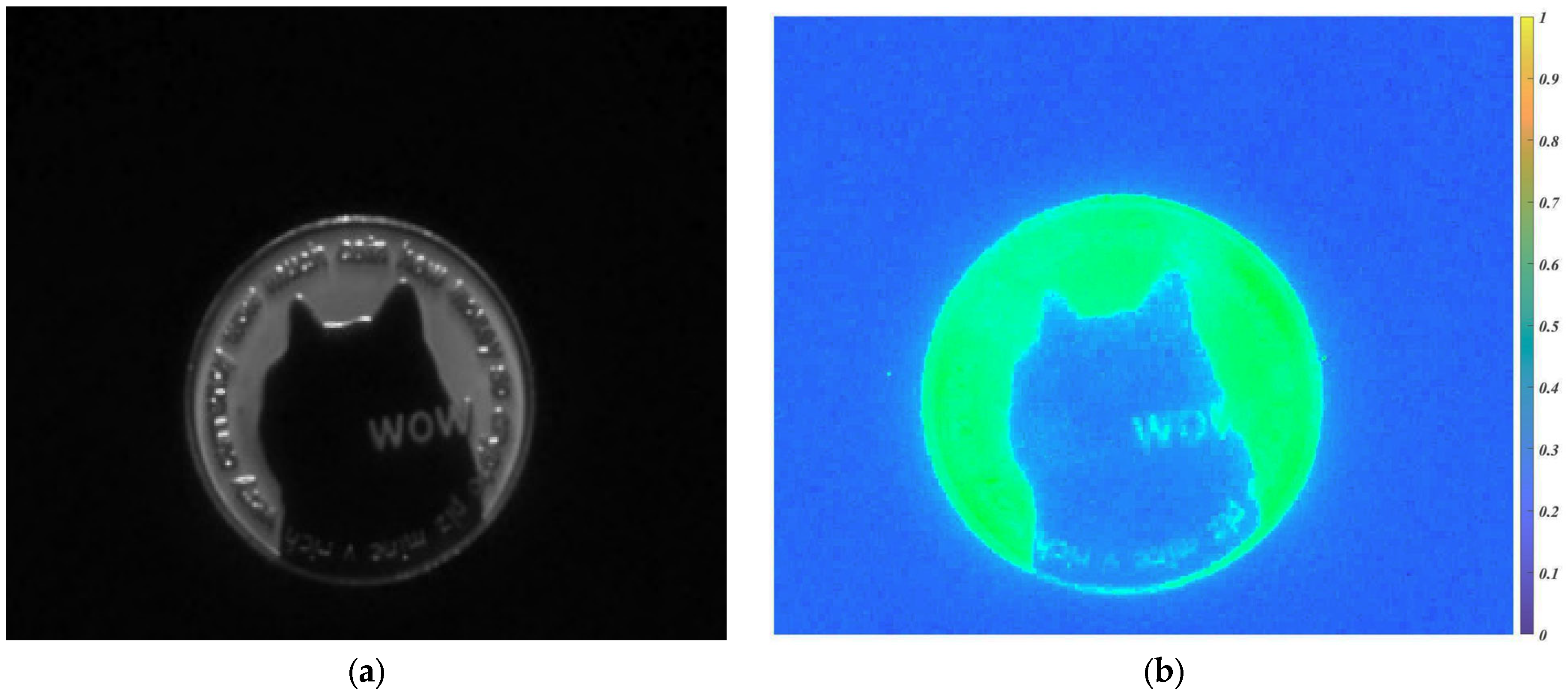
2.3. Analysis and Extraction of Low and High Polarization Regions
2.4. Polarization Difference Recovery in Low Polarization Region
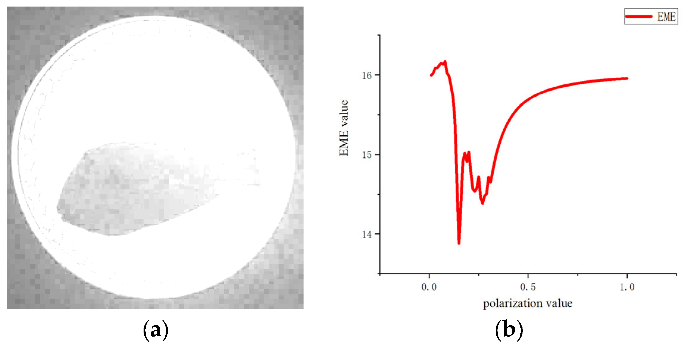
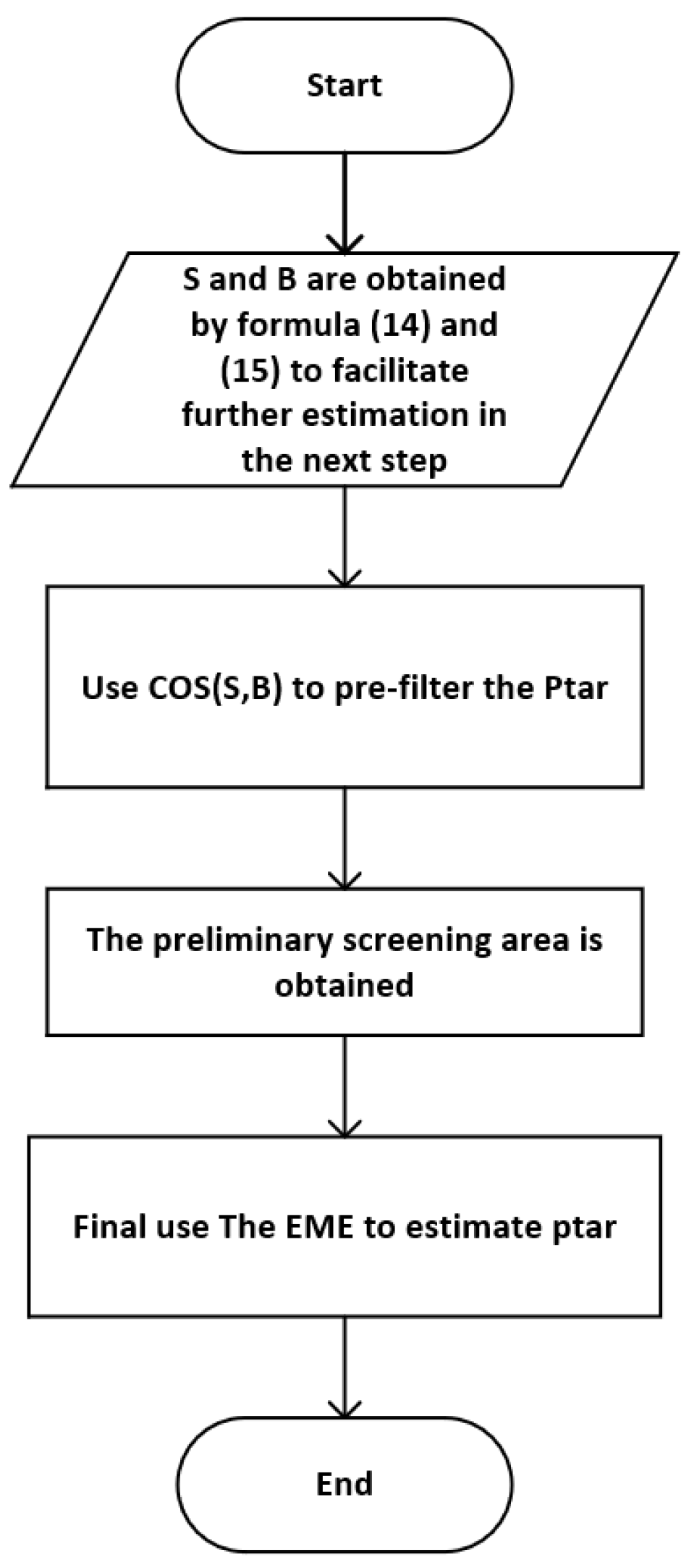
2.5. Joint Estimation of Target Light Polarization
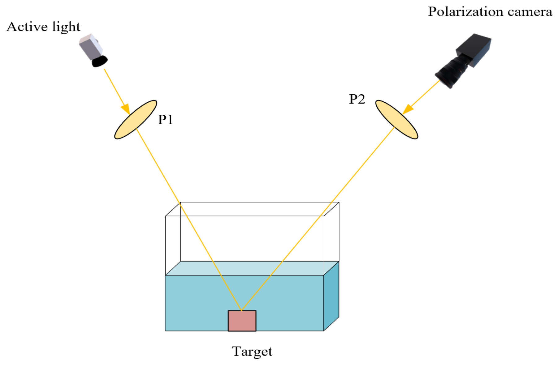
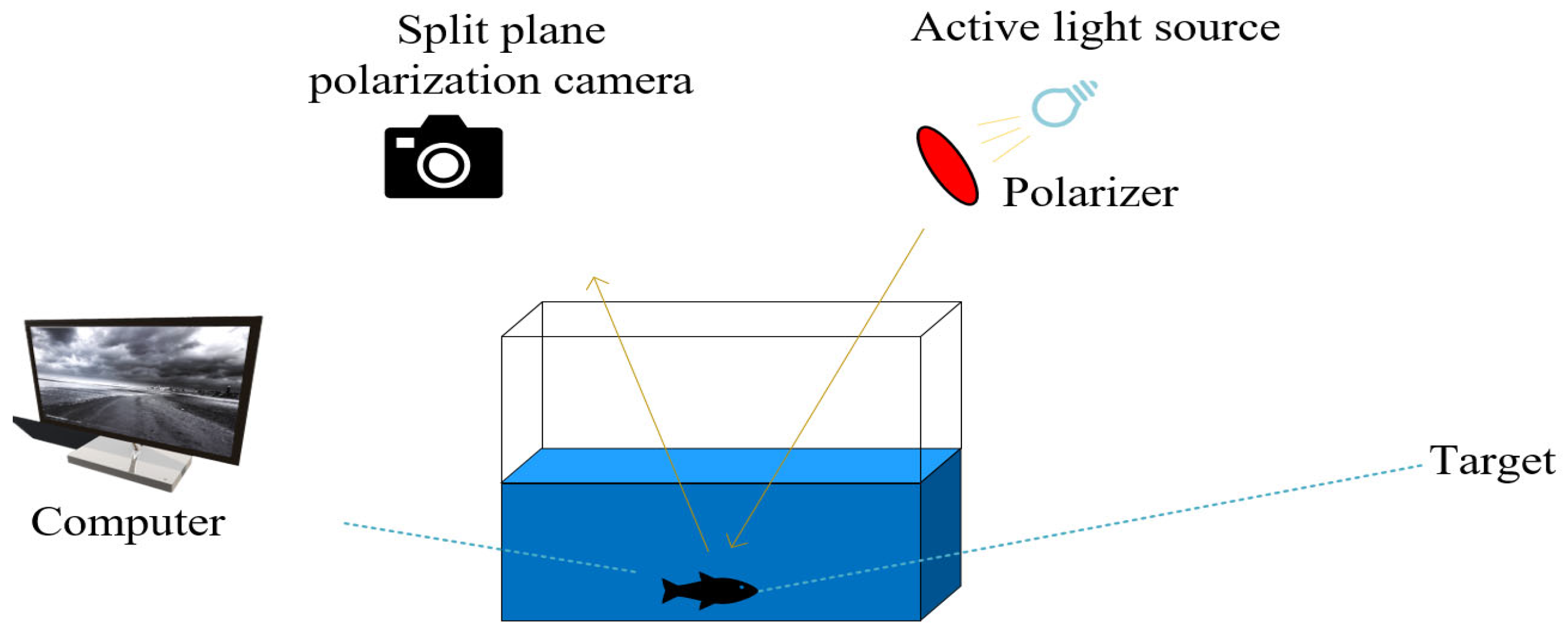
2.6. Experimental Environment
3. Experimental Results and Discussion
4. Conclusions
Author Contributions
Funding
Institutional Review Board Statement
Informed Consent Statement
Data Availability Statement
Conflicts of Interest
References
- Yuan, X.; Guo, L.X.; Luo, C.T.; Zhao, X.T.; Yu, C.T. A Survey of Target Detection and Recognition Methods in Underwater Turbid Areas. Appl. Sci. 2022, 12, 4898. [Google Scholar] [CrossRef]
- Hu, K.; Weng, C.H.; Zhang, Y.W.; Jin, J.L.; Xia, Q.F. An Overview of Underwater Vision Enhancement: From Traditional Methods to Recent Deep Learning. J. Mar. Sci. Eng. 2022, 10, 241. [Google Scholar] [CrossRef]
- Guo, J.C.; Li, C.Y.; Guo, C.L.; Chen, S.J. Research progress of underwater image enhancement and restoration methods. J. Image Graph. 2017, 22, 273–287. [Google Scholar] [CrossRef]
- Zhao, Y.Q.; Dai, H.M.; Shen, L.H. Review of underwater polarization clear imaging methods. Infrared Laser Eng. 2020, 49, 43–53. [Google Scholar] [CrossRef]
- Bazeille, S.; Quidu, I.; Jaulin, L.; Malkasse, J.-P. Automatic underwater image pre-processing. In Proceedings of the CMM’06, Brest, France, 16–19 October 2006. [Google Scholar]
- He, K.M.; Sun, J.; Tang, X.O. Single image haze removal using dark channel prior. In Proceedings of the IEEE Transactions on Pattern Analysis and Machine Intelligence, Miami, FL, USA, 18 August 2009. [Google Scholar] [CrossRef]
- Galdran, A.; Pardo, D.; Picón, A. Automatic Red-Channel underwater image restoration. J. Vis. Commun. Image Represent. 2015, 26, 132–145. [Google Scholar] [CrossRef]
- Zhang, H.J.; Gong, J.R.; Ren, M.Y.; Zhou, N.; Wang, H.T.; Meng, Q.G.; Zhang, Y. Active Polarization Imaging for Cross-Linear Image Histogram Equalization and Noise Suppression in Highly Turbid Water. Photonics 2023, 10, 145. [Google Scholar] [CrossRef]
- Schechner, Y.Y.; Karpel, N. Recovery of underwater visibility and structure by polarization analysis. IEEE J. Ocean. Eng. 2005, 30, 102–119. [Google Scholar] [CrossRef]
- Schechner, Y.Y.; Karpel, N. Clear underwater vision. In Proceedings of the IEEE Conference on Computer Vision and Pattern Recognition, Washington, DC, USA, 19 July 2004. [Google Scholar] [CrossRef]
- Huang, B.J.; Liu, T.G.; Hu, H.F.; Han, J.F.; Yu, M.X. Under-water image recovery considering polarization effects of objects. Opt. Express 2016, 24, 9826–9838. [Google Scholar] [CrossRef] [PubMed]
- Hu, H.F.; Zhao, L.; Huang, B.J.; Li, X.B.; Wang, H.; Liu, T.G. Enhancing Visibility of Polarimetric Underwater Image by Transmittance Correction. IEEE Photonics J. 2017, 9, 6802310. [Google Scholar] [CrossRef]
- Li, H.X.; Zhu, J.P.; Deng, J.X.; Guo, F.Q.; Zhu, J.P. Visibility enhancement of underwater images based on polarization common-mode rejection of a highly polarized target signal. Opt. Express 2022, 30, 43973–43986. [Google Scholar] [CrossRef] [PubMed]
- Zhang, H.J.; Zhou, N.; Meng, Q.G.; Guo, F.Q.; Ren, M.Y.; Wang, H.T. Local optimum underwater polarization imaging enhancement based on connected domain prior. J. Opt. 2022, 24, 10570. [Google Scholar] [CrossRef]
- Li, R.H.; Zhang, S.H.; Cai, C.; Xu, Y.; Cao, H. Underwater polarization image restoration based on a partition method. Opt. Eng. 2023, 62, 068103. [Google Scholar] [CrossRef]
- Li, R.H.; Cai, C.Y.; Zhang, S.H.; Xu, Y.H.; Cao, H.T. Polarization parameter partition optimization restoration method for underwater degraded image. Opt. Precis. Eng. 2023, 31, 3010. [Google Scholar] [CrossRef]
- Wang, J.J.; Wan, M.J.; Cao, X.Q.; Zhang, X.J.; Gu, G.H.; Chen, Q. Active non-uniform illumination-based underwater polarization imaging method for objects with complex polarization properties. Opt. Express 2022, 19, 46926–46943. [Google Scholar] [CrossRef] [PubMed]
- Li, X.B.; Hu, H.F.; Zhao, L.; Wang, H.; Yu, Y.; Wu, L. Polarimetric image recovery method combining histogram stretching for underwater imaging. Sci. Rep. 2018, 8, 12430. [Google Scholar] [CrossRef] [PubMed]
- Shi, C.Y.; Zhu, Z.W.; Yin, G.F.; Gao, X.H.; Wang, Z.M.; Zhang, S.; Zhou, Z.H.; Hu, X.Y. Measurement of Submicron Particle Size Using Scattering Angle-Corrected Polarization Difference with High Angular Resolution. Photonics 2023, 10, 1282. [Google Scholar] [CrossRef]
- Miao, Y.; Sowmya, A. New image quality evaluation metric for underwater video. IEEE Signal Lett. 2014, 21, 1215–1219. [Google Scholar] [CrossRef]
- Agaian, S.S.; Panetta, K.; Grigoryan, A.M. Transform-based image enhancement algorithms with performance measure. IEEE Trans. Image Process. 2001, 10, 367–382. [Google Scholar] [CrossRef] [PubMed]
- Treibitz, T.; Schechner, Y.Y. Active polarization descattering. IEEE Trans. PAMI 2009, 31, 385–399. [Google Scholar] [CrossRef] [PubMed]
- Han, P.; Li, X.; Liu, F.; Cai, Y.; Yang, K.; Yan, M.; Sun, S.; Liu, Y.; Shao, X. Accurate passive 3D polarization face reconstruction under complex conditions assisted with deep learning. Photonics 2022, 9, 924. [Google Scholar] [CrossRef]

| Camera Sensor Resolution | 2248 × 2048 px, 5.0 MP |
| operating temperature | −20 to 50 °C |
| active light | Rawray 150 W LED Light |
| linearly polarized light | USP-50C0.4-38 |
| High-Transparency Acrylic Tank | 40 cm, 40 cm, 50 cm with over 96% light transmission |
| software platform | matlab2020a |
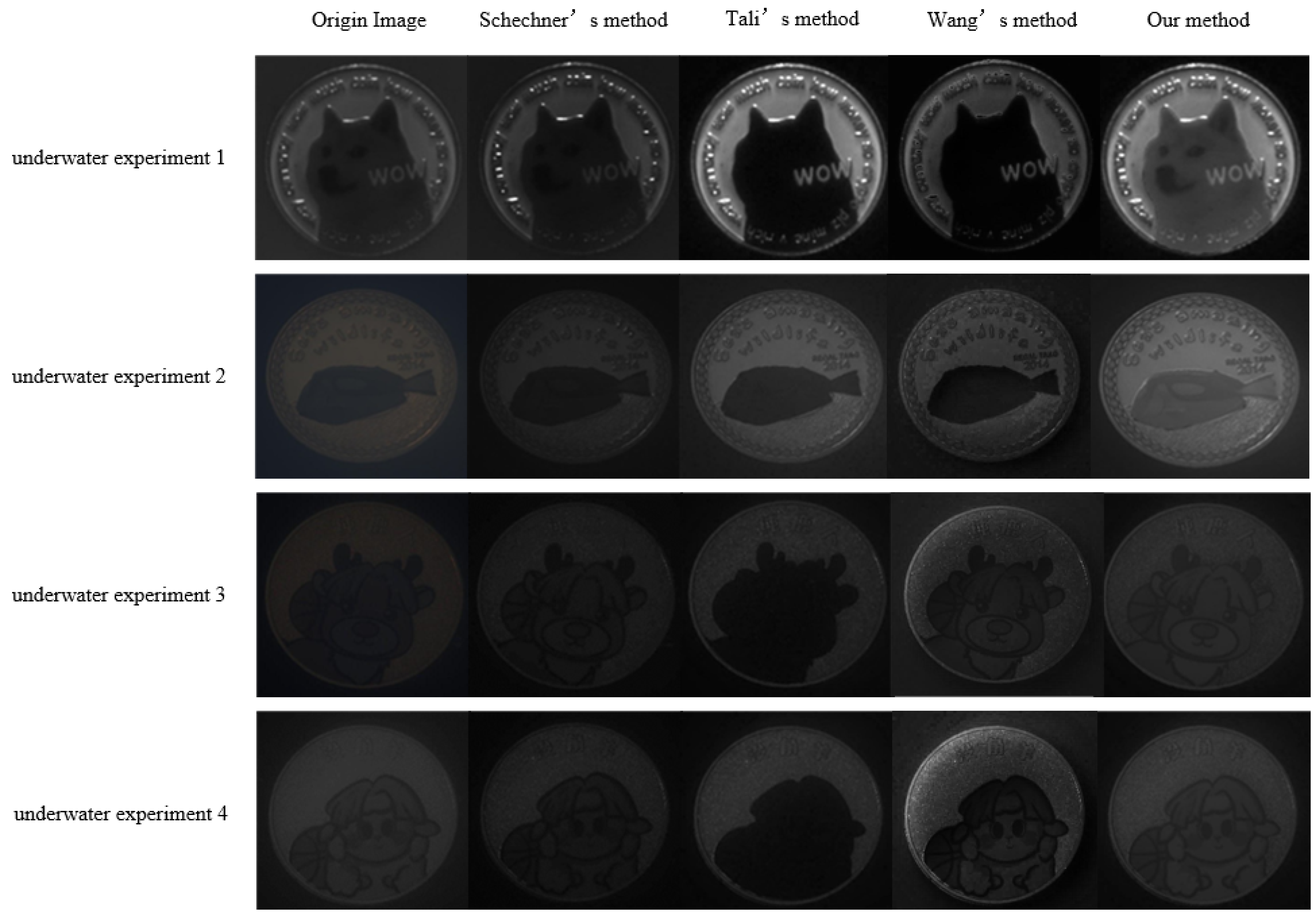
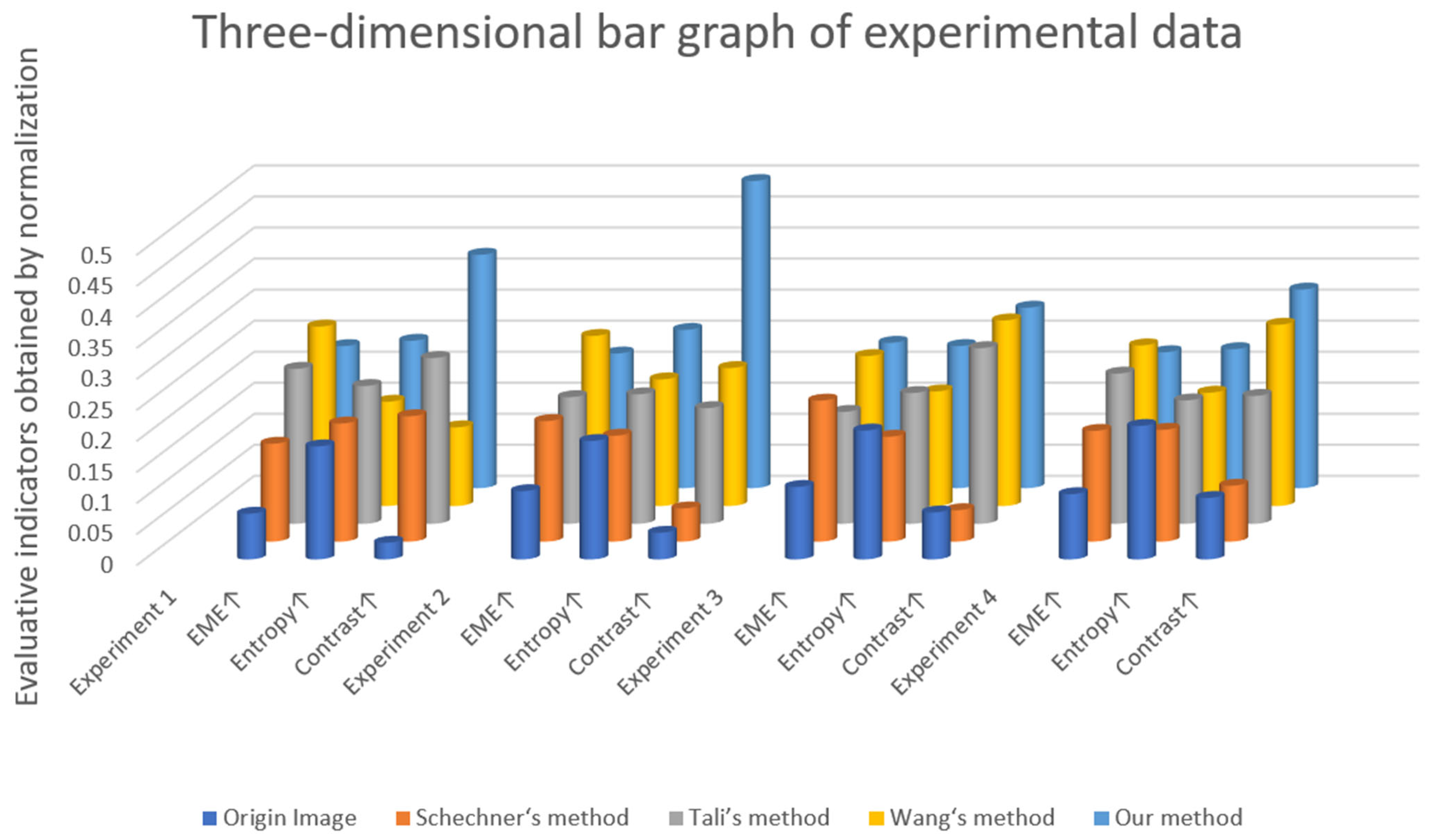
| Underwater Experiment 1 | Joint Evaluation Indicators | ||
|---|---|---|---|
| EME ↑ | Entropy ↑ | Contrast ↑ | |
| Origin Image | 6.026 | 5.180 | 3.216 |
| Schechner‘s method | 12.912 | 5.412 | 24.318 |
| Tali’s method | 20.443 | 6.312 | 32.048 |
| Wang‘s method | 23.734 | 4.777 | 15.181 |
| Our method | 18.727 | 6.751 | 45.058 |
| Underwater Experiment 2 | Joint Evaluation Indicators | ||
| EME ↑ | Entropy ↑ | Contrast ↑ | |
| Origin Image | 4.504 | 5.305 | 2.253 |
| Schechner‘s method | 7.941 | 4.748 | 2.812 |
| Tali’s method | 8.349 | 5.799 | 9.790 |
| Wang‘s method | 11.214 | 5.692 | 11.673 |
| Our method | 8.867 | 6.255 | 25.987 |
| Underwater Experiment 3 | Joint Evaluation Indicators | ||
| EME ↑ | Entropy ↑ | Contrast ↑ | |
| Origin Image | 2.528 | 4.738 | 1.202 |
| Schechner‘s method | 4.916 | 3.866 | 0.803 |
| Tali’s method | 3.902 | 4.808 | 4.491 |
| Wang‘s method | 5.226 | 4.210 | 4.654 |
| Our method | 5.067 | 5.193 | 4.615 |
| Underwater Experiment 4 | Joint Evaluation Indicators | ||
| EME ↑ | Entropy ↑ | Contrast ↑ | |
| Origin Image | 2.130 | 5.363 | 2.242 |
| Schechner‘s method | 3.614 | 4.490 | 2.034 |
| Tali’s method | 4.902 | 4.955 | 4.648 |
| Wang‘s method | 5.239 | 4.550 | 6.585 |
| Our method | 4.365 | 5.560 | 7.029 |
Disclaimer/Publisher’s Note: The statements, opinions and data contained in all publications are solely those of the individual author(s) and contributor(s) and not of MDPI and/or the editor(s). MDPI and/or the editor(s) disclaim responsibility for any injury to people or property resulting from any ideas, methods, instructions or products referred to in the content. |
© 2024 by the authors. Licensee MDPI, Basel, Switzerland. This article is an open access article distributed under the terms and conditions of the Creative Commons Attribution (CC BY) license (https://creativecommons.org/licenses/by/4.0/).
Share and Cite
Cai, C.; Fan, Y.; Li, R.; Cao, H.; Zhang, S.; Wang, M. Underwater Degraded Image Restoration by Joint Evaluation and Polarization Partition Fusion. Appl. Sci. 2024, 14, 1769. https://doi.org/10.3390/app14051769
Cai C, Fan Y, Li R, Cao H, Zhang S, Wang M. Underwater Degraded Image Restoration by Joint Evaluation and Polarization Partition Fusion. Applied Sciences. 2024; 14(5):1769. https://doi.org/10.3390/app14051769
Chicago/Turabian StyleCai, Changye, Yuanyi Fan, Ronghua Li, Haotian Cao, Shenghui Zhang, and Mianze Wang. 2024. "Underwater Degraded Image Restoration by Joint Evaluation and Polarization Partition Fusion" Applied Sciences 14, no. 5: 1769. https://doi.org/10.3390/app14051769
APA StyleCai, C., Fan, Y., Li, R., Cao, H., Zhang, S., & Wang, M. (2024). Underwater Degraded Image Restoration by Joint Evaluation and Polarization Partition Fusion. Applied Sciences, 14(5), 1769. https://doi.org/10.3390/app14051769