Improved Temporal Fuzzy Reasoning Spiking Neural P Systems for Power System Fault Diagnosis


Abstract
1. Introduction
- The ITFRSNP system and its associated reasoning algorithm are proposed. The ITFRSNP system contains new rule neurons and reasoning methods, simplifying the correlation reasoning of confidence degrees and temporal features. The ITFRSNP system can effectively improve the accuracy and fault tolerance of fault diagnosis. This lays a theoretical foundation for constructing a general fault diagnosis model and its diagnosis reasoning method.
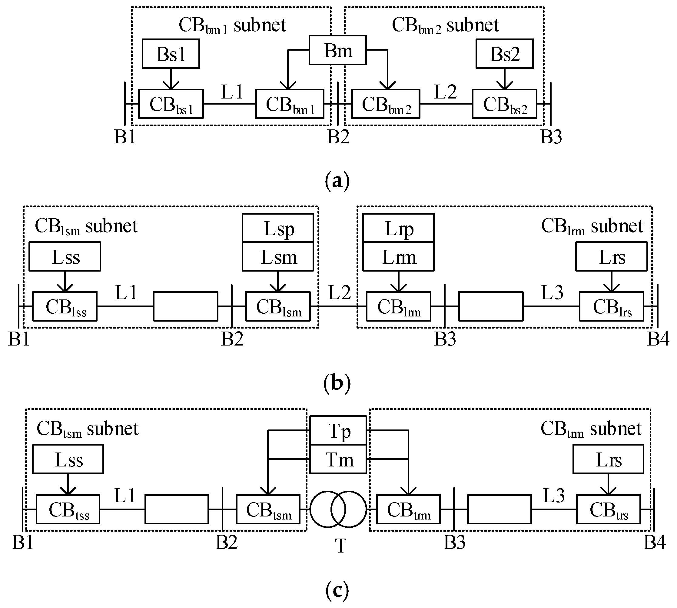
- The CB subnet is defined based on the configuration of the CBs and corresponding protections. A general fault diagnosis model and its fault diagnosis process are developed based on the ITFRSNP system for CB subnets. The proposed model simplifies the modeling process and can be directly applied to fault diagnosis of various components with good versatility and adaptability.
- A search method for suspected faulty components is proposed. The search method does not need to traverse the entire power system and does not miss suspected faulty components. This method narrows the scope of topology search and fault diagnosis and can effectively improve the efficiency of fault diagnosis.
2. ITFRSNP System
2.1. Temporal Constraints and Temporal Reasonings
- The time-point constraint (T(a) = [ta−, ta+]) indicates that event a occurs in the time interval [ta−, ta+]. If ta− = ta+, event a occurs at a specific time.
- The time-distance constraint (D(a, b) = [Δtab−, Δtab+]) indicates that the time distance between the occurrence times of events a and b is within the time interval [Δtab−, Δtab+].
- Reverse reasoning: The time-point constraint T(b) and the time-distance constraint D(a, b) are known. The following definition can be employed to infer the time-point constraint T(a):
- Merge reasoning: If event a is known to satisfy multiple time-point constraints T1(a), T2(a), T3(a), …, Tk(a) simultaneously, the following definition can be employed to infer the time-point constraint T(a).
2.2. The TFRSNP System
- A = {a} is a singleton alphabet (a is called spike).
- Np = {σp1, σp2, …, σpm} denotes the proposition neuron set, where σpi (1 ≤ i ≤ m) is associated with a fuzzy proposition. Each proposition neuron σpi has the form σpi = (αpi, Tpi, θpi, λpi, rpi), where the following are defined:
- αpi (αpi ∈ [0, 1]) is the spike value in σpi;
- Tpi (Tpi = [tpi−, tpi+]) is the time-point constraint in σpi;
- θpi is an integer representing the number of spikes received by σpi;
- λpi is an integer that represents the spike number threshold required for firing σpi;
- rpi is a firing/spiking rule of σpi with the form E/aθ → aβ, where θ and β are real numbers in [0, 1].
- Nr = {σr1, σr2, …, σrn} is the rule neuron set, where σrj (1 ≤ j ≤ n) is associated with a fuzzy production rule. Nr contains two types of rule neurons: TIME-type and OR-type. Each rule neuron σrj has the form σrj = (αrj, Trj, Drj, θrj, λrj, rrj), where:
- αrj (αrj ∈ [0, 1]) is the spike value in σrj;
- Trj (Trj = [trj−, trj+]) is the time-point constraint in σrj;
- Drj (Drj = [Δtrj−, Δtrj+]) is the time-distance constraint in σrj, which denotes the time-distance constraint between the propositions of the input and output proposition neurons associated with σrj;
- θrj is an integer representing the number of spikes received by σrj;
- λrj is an integer that represents the spike number threshold required for firing σrj;
- rrj is a firing/spiking rule of σrj, with the form E/aθ→ aβ, where θ and β are real numbers in [0, 1].
- is a directed graph that indicates the synapses between propositions and rule neurons. Input matrices U1 = {u1(i, j)}m×n and U2 = {u2(i, j)}m×n and output matrix V = {v(j, i)}n×m, where u1(i, j), u2(i, j), and v(i, j) ∈ [0, 1], are used to represent syn. If there is a synapse from proposition neuron σpi to TIME-type neuron σrj, then u1(i, j) = 1; otherwise, u1(i, j) = 0. If there is a synapse from proposition neuron σpi to OR-type neuron σrj, then u2(i, j) = 1; otherwise, u2(i, j) = 0. If there is a directed arc (synapse) from rule neuron σrj to proposition neuron σpi, then v(j, i) = 1; otherwise, v(j, i) = 0.
- I and O are input and output neuron sets, respectively.
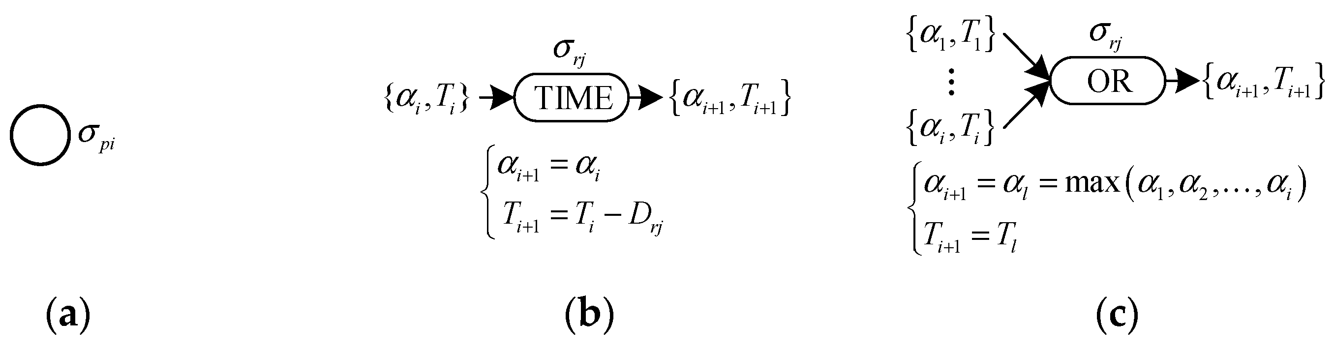
- The proposition neuron (Figure 1a) describes the operational events of PRs and CBs. When a PR alarm message is received, the spike value in the proposition neuron corresponds to its confidence degree, and the time-point constraint corresponds to its operation time. The proposition neuron can delineate the state and time of the PR and CB operations, which are then inputted into the fault diagnosis model for inference. Moreover, this neuron can record the intermediate and output results of the fault diagnosis.
- The TIME-type rule neuron (Figure 1b) receives spikes from the proposition neuron. It then transmits the spike value to the next proposition neuron, and deduces the time-point constraints backward according to Equation (1) before forwarding them. This rule neuron is responsible for characterizing the temporal distance constraints between propositions that correspond to their associated propositional neurons. The TIME-type rule neurons employ reverse reasoning to deduce the time-point constraints for the PRs from those of the corresponding CBs and their time-distance constraints. Similarly, they apply to determine the time-point constraints of the faults by leveraging the time-point constraints and time-distance constraints of the PRs.
- The OR-type rule neuron (Figure 1c) receives spikes from the proposition neurons and takes the maximum spike value αl and the corresponding time-point constraint Tl to transmit to the next proposition neuron. Each component is equipped with multiple sets of protections, including primary, near backup, and remote backup protections. The OR-type rule neuron determines the protection type for isolating the faulty component by selecting the PR and CB with the highest confidence degree.
2.3. The Reasoning Algorithm of the ITFRSNP System
- αp = (αp1, αp2, …, αpm)T and αr = (αr1, αr2, …, αrn)T are vectors consisting of spike values in m proposition and n rule neurons, respectively. αpi (1 ≤ i ≤ m) and αrj (1 ≤ j ≤ n) represent the spike values of the i-th proposition neuron and j-th rule neuron, respectively. This relationship between the vector elements and neurons applies to the subsequent vector definitions as well.
- Tp = (Tp1, Tp2, …, Tpm)T and Tr = (Tr1, Tr2, …, Trn)T are vectors consisting of time-point constraints in m proposition and n rule neurons, respectively.
- Dr = (Dr1, Dr2, …, Drn)T is a vector of the time-distance constraints in n rule neurons.
- θp = (θp1, θp2, …, θpm)T and θr = (θr1, θr2, …, θrn)T are vectors consisting of spike numbers in m proposition and n rule neurons, respectively.
- λp = (λp1, λp2, …, λpm)T and λr = (λr1, λr2, …, λrn)T are vectors consisting of spike number thresholds in m proposition and n rule neurons, respectively.
- βp = (βp1, βp2, …, βpm)T and βr = (βr1, βr2, …, βrn)T are vectors consisting of spike values output from m proposition neurons and n rule neurons, respectively.
- τp = (τp1, τp2, …, τpm)T and τr = (τr1, τr2, …, τrn)T are vectors consisting of time-point constraints output from m proposition and n rule neurons, respectively, after firing.
- bp = (bp1, bp2, …, bpm)T and br = (br1, br2, …, brn)T are vectors consisting of spike numbers output from m proposition neurons and n rule neurons, respectively, after firing.
- Bp = diag(bp) and Br = diag(br) are diagonal matrices, where diag( ) is the diagonal function.
- H = CD:where D and H are t × 1-and s × 1-dimensional vectors of time-distance constraints, respectively, and C is an s × t-dimensional binary matrix.
- J = GH:where G and J are s × 1-dimensional vectors of time-point constraints.
- {P, Q} = {C, D}{F, G}:where F and P are s × 1 and t × 1-dimensional vectors of spike values, and Q is a t × 1-dimensional vector of time-point constraints.
- {P, Q} = {C,D} {F,G}:
- {P, Q} = {,}{,}:where and are t × 1-dimensional vectors of the spike values, and and are t × 1-dimensional vectors of the time-point constraints.
- {P, Q} = {,}{,}:
- {β,τ} = fire (α, T, θ, λ):
- {α,T} = update (α, T, θ, λ):
- b = fire (1, θ, λ):
- θ = update (θ, θ, λ):
- Input parameter matrices and vectors U1, U2, V, λp, λr, Dr, θp, and θr. The number of interactive inferences is g, and the vectors of the spike values and time-point constraints in the g-th iteration are , , , and . Initialize the number of iterations g = 0 and input , , , and .
- Process the firing of proposition neurons:
- Compute , and :
- Process the firing of rule neurons:
- Compute , and :
- If = (0, 0, …, 0)T and = (0, 0, …, 0)T, then halt and export reasoning results ( and ); otherwise, g = g + 1 and return to Step 2.
2.4. Comparison between ITFRSNP and RTSSNPS Systems
3. ITFRSNP System-Based General Fault Diagnosis Model and Its Fault Diagnosis Process
3.1. ITFRSNP System-Based General Fault Diagnosis Model and Fault Diagnosis Principle
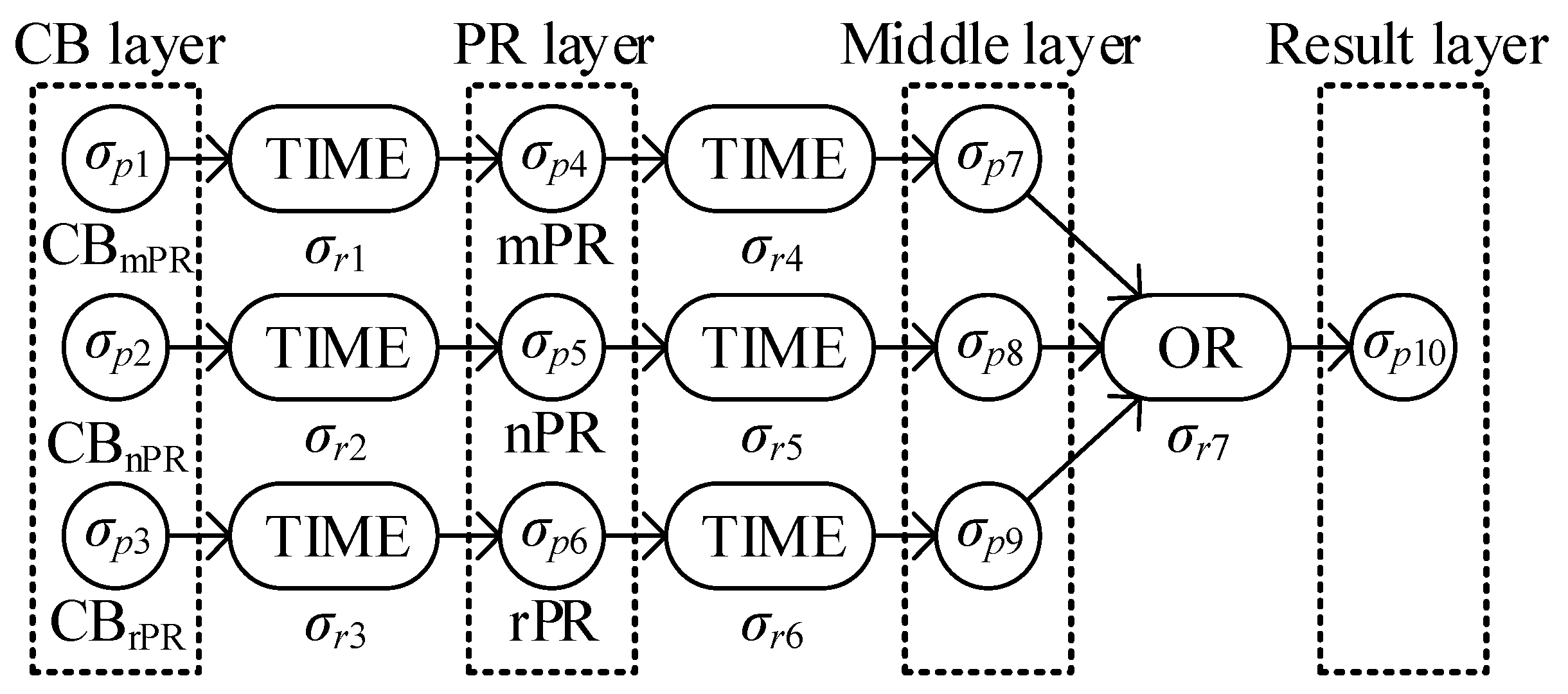
- σp1, σp2, and σp3 fire, and the confidence degrees and time-point constraints of the CBs are input into σr1, σr2, and σr3.
- σr1, σr2, and σr3 infer the time-point constraints of the PRs according to the time-point constraints and time-distance constraints of the CBs. Then, σr1, σr2, and σr3 fire, and the confidence degrees of the CBs and the temporal reasoning results of the PRs are input into σp4, σp5, and σp6.
- σp4, σp5, and σp6 fuse the confidence degrees of the PRs and CBs, and the temporal reasoning results from σp4, σp5, and σp6 are matched with the time-point constraints of the PRs in σp4, σp5, and σp6. Then, σp4, σp5, and σp6 fire, and the confidence fusion results and temporal matching results are input into σr4, σr5, and σr6.
- σr4, σr5, and σr6 infer the fault time based on the temporal matching results and the time-distance constraints of the PRs. Then, σr4, σr5, and σr6 fire, and the confidence fusion results and temporal reasoning results of the fault time are input into σp7, σp8, and σp9. Finally, σp7, σp8, and σp9 fire, these results are input into σr7.
- σr7 is responsible for selecting the highest confidence degree among σp7, σp8, and σp9 and its time-point constraints as the diagnosis result of the subnet output into σp10.
3.2. Model Parameters of the General Fault Diagnosis Model
- The input matrices U1 and U2, and the output matrix V of the general fault diagnosis model are as follows:where I is the unit matrix, O is the zero matrix, and E is the matrix with all the elements equal to 1.
- If the PR/CB operation time is t0, the time-point constraint of the related proposition neuron is [t0, t0]. For PR/CB without an alarm message, the time-point constraint of the related proposition neuron is .
- The time-distance constraints for the bus PR, main PR, near backup PR, and remote backup PR are [10, 40] ms, [10, 40] ms, [310, 340] ms, and [510, 540] ms relative to the fault time, respectively. The time-distance constraint for the CB is [20, 40] ms relative to the protection operation time. Therefore, the vector Dr of the general fault diagnosis model is as follows:
- The spike numbers of the proposition neurons in the PR and CB layers are set to 1, and the spike numbers of the other neurons are set to zero to ensure that spikes from proposition neurons can be delivered to rule neurons. Therefore, the vectors θp and θr of the general fault diagnosis model are as follows:
- Because the PR layer neurons need to obtain spikes from the CB layer neurons to fire, the spike number thresholds of all proposition neurons in the PR layer are set to two, and the spike number thresholds of other proposition neurons are set to one. Rule neurons must obtain spikes from all input proposition neurons to fire; therefore, their spike number thresholds are equal to the number of their input proposition neurons. Therefore, the vectors λp and λr of the general fault diagnosis model are as follows:
3.3. ITFRSNP System-Based General Fault Diagnosis Process
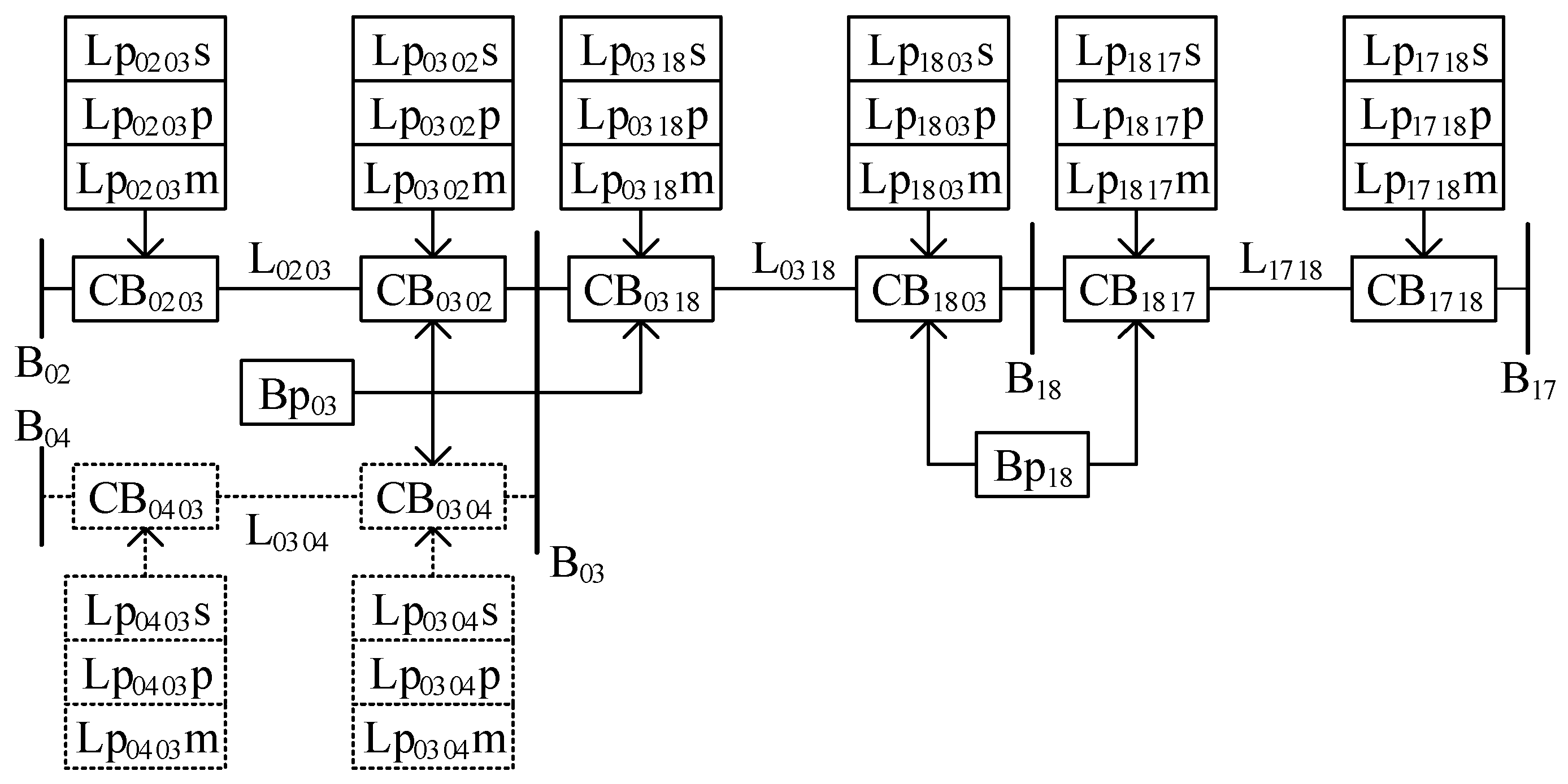
3.3.1. Suspected Faulty Component Search Method
- Alarm messages are received from the W CBs. These CBs form the CB set (CBS). Initialize w = 1 and begin the search.
- Select the w-th CB (CBw) in CBS.
- Buses, lines, and transformers connected to CBw are searched to form the w-th subset of suspected faulty components (COMw).
- Adjacent buses, lines and transformers are searched in the direction of the line or transformer connected to the CBw and placed into COMw.
- If w = W, proceed to the next step; otherwise, w = w + 1 and return to Step 3.
- The suspected faulty component subsets intersect in pairs. If the intersection of two suspected faulty components is not empty, then the intersection results are combined into a total set of suspected faulty components (COMS). If the intersection of a certain suspected faulty component subset with other subsets is empty, all the components in this subset are input into COMS. The components in COMS are suspected to be faulty components.
3.3.2. Fault Diagnosis Process
- After receiving the alarm messages, start the search method for suspected faulty components and set the total number of suspected faulty components as X. Initialize x = 1.
- Select the x-th suspected faulty component and set the number of CBs connected to it as Y. Initialize y = 1.
- Initialize the general fault diagnosis model with neuron spike values of zero and time-point constraints of . The y-th CB is selected for search. If the x-th suspected faulty component is a line or transformer, search for the main PR and near-backup PR corresponding to the CB. If the x-th suspected faulty component is a bus, the bus PR corresponding to the CB is searched. According to the alarm messages, σp1, σp2, σp4, and σp5 in the general fault diagnosis model are assigned spike values and time-point constraints concerning Section 3.1.
- The number of adjacent lines of the y-th CB is set as Z. If Z = 0, skip to Step 8; otherwise, initialize z = 1.
- The initial values of nCBrPR.o, nCBrPR.c, nrPR.o, and nrPR.c are 0; the initial values of TCBrPR.oi and TrPR.oi are . Search for CBs at the far end of the z-th adjacent line. If the CB has an alarm message at tCBrPRz, then nCBrPR.o = nCBrPR.o + 1, and TCBrPR = TCBrPR ∪ [tCBrPRz, tCBrPRz]; otherwise, nCBrPR.c = nCBrPR.c + 1. Search for the remote backup PR corresponding to the CB at the far end of the z-th adjacent line, and if this remote backup PR has an alarm message at trPRz, then nrPR.o = nrPR.o + 1 and TrPR = TrPR ∪ [trPRz, trPRz]; otherwise, nrPR.c = nrPR.c + 1.
- If z < Z, z = z + 1, and return to Step 5; otherwise, substitute nCBrPR.o, nCBrPR.c, nrPR.o, nrPR.c, TCBrPR, and TrPR into (21) to yield αp3, Tp3, αp6, and Tp6.
- Based on the parameter definitions in Section 2.3, the inputs ( and ) are determined for the general fault diagnosis model corresponding to the y-th CB subnet of the x-th suspected faulty component. The reasoning algorithm in Section 2.3 is introduced to obtain the diagnosis result (αp10(xy) and Tp10(xy) of σp10) for the y-th CB subnet.
- If y < Y, then y = y + 1 and return to Step 3; otherwise, the diagnosis results (α(x) and T(x)) of the x-th suspected faulty component are obtained by substituting the diagnosis results of the subnets of this component into the following equations:
- The measured value η(x) of the x-th suspected faulty component is obtained by substituting α(x) and T(x) into the measurement function, as shown in Equation (29). The threshold of the measured value was set to 0.6, considering the uncertainty and timestamp errors of the alarm messages. A component is faulty if η(x) is greater than 0.6.
- If x < X, then x = x + 1 and return to Step 2; otherwise, complete the fault diagnosis for all suspected faulty components and end the fault diagnosis process.
4. Case Studies
4.1. Fault Case Analysis
4.1.1. Case 1 (Bus Fault)
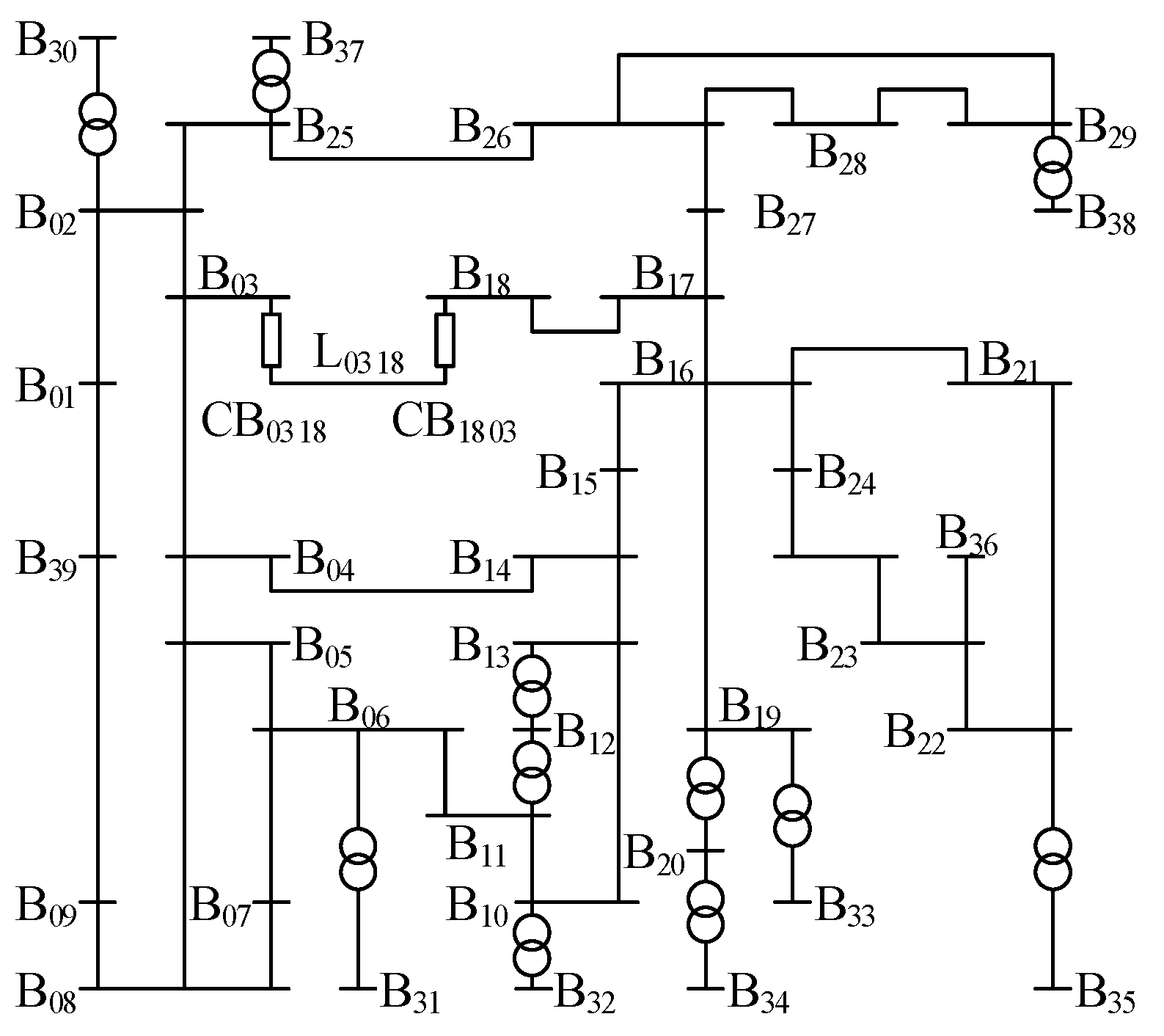
- CBS = {CB1817, CB1803} can be obtained from the alarm message. Traverse CBS and search for suspected faulty components. There are a subset COM1817 = {B18, L1817, B17, L1727, L1617}, a subset COM1803 = {B18, L0318, B03, L0203, L0304}, and a total set COMS = {B18}.
- B18 is selected for fault diagnosis. CB1803 connected to B18 is selected for the search, and its corresponding bus PR is Bp18, respectively. According to the alarm messages, the spike values of σp1, σp2, σp4, and σp5 are 0.9833, 0.85, 0.8564, and 0, respectively, and their time-point constraints are [40, 40], [40, 40], [0, 0], and , respectively.
- The adjacent line corresponding to CB0318 is L0318, the CB at the far end is CB0318, and the remote backup PR is Lp0318s. Because the alarm information is not received from the above PRs and CBs, nCBrPR.o = 0, nCBrPR.c = 1, TCBrPR = , nrPR.o = 0, nrPR.c = 1, and TrPR = . Substituting them into (21) to obtain the spike values and time-point constraints for σp3 and σp6 are 0.2 and , respectively.
- and of the fault diagnosis model for the CB1803 subnet are as follows:
- , and model parameters are imported into the reasoning algorithm, the diagnosis results of the CB1803 subnet are αp10(11) = 0.9199, Tp10(11) = [−40, −10].
- Similarly, and of the fault diagnosis model for the CB1817 subnet are as follows:
- Similarly, the diagnosis results for the CB1817 subnet are αp10(12) = 0.9199 and Tp10(12) = [−40, −10].
- αp10(11), Tp10(11), αp10(12) and Tp10(12) are substituted into (28), and the diagnosis results α(1) = 0.9199 and T(1) = [−40, −10] for B18. α(1) and T(1) are substituted into (29), and the measured value of B18 is η(1) = 0.9439, which is greater than 0.6. Therefore, B18 is a faulty component.
4.1.2. Case 2 (Line Fault with the CB Rejection)
- Based on the alarm messages, COMS = {L0318, L1718, B18} is obtained.
- L0318 is selected for fault diagnosis. The , , , and of the fault diagnosis model for the CB0318 and CB1803 subnets are as follows.
- The diagnosis results for the CB0318 subnet are αp10(11) = 0.9873 and Tp10(11) = [−38, −8]. The diagnosis results of the CB1803 subnet are αp10(12) = 0.725 and Tp10(12) = [−20, 10]. The diagnosis results of L0318 are α(1) = 0.8562 and T(1) = [−20, 10], and its measured value is η(1) = 0.8993, which is greater than 0.6. Thus, L0318 is a faulty component.
- Similarly, the measured values of L1718 and B18 are 0.3733 and 0.42, respectively, and L1718 and B18 are non-faulty components.
4.1.3. Case 3 (Transformer Fault with Missing CB Alarm Message)
- Based on the alarm messages, COMS = {T1213, B12, B13, L1314, L1013} is obtained.
- T1213 is selected for fault diagnosis. The , , , and of the fault diagnosis model for the CB1312 and CB1213 subnets are as follows.
- The diagnosis results for the CB1312 subnet are αp10(11) = 0.4878 and Tp10(11) = [−40, −10]. The diagnosis results of the CB1213 subnet are αp10(12) = 0.8795 and Tp10(12) = [−40, −10]. The diagnosis results of T1213 are α(1) = 0.6836 and T(1) = [−40, −10], and its measured value η(1) = 0.7785, which is greater than 0.6. Thus, T1213 is a faulty component.
- Similarly, the measured values of B12, B13, L1314, and L1013 are 0.2771, 0.2042, 0.1881, and 0.1881, respectively, and they are non-faulty components.
4.1.4. More Cases
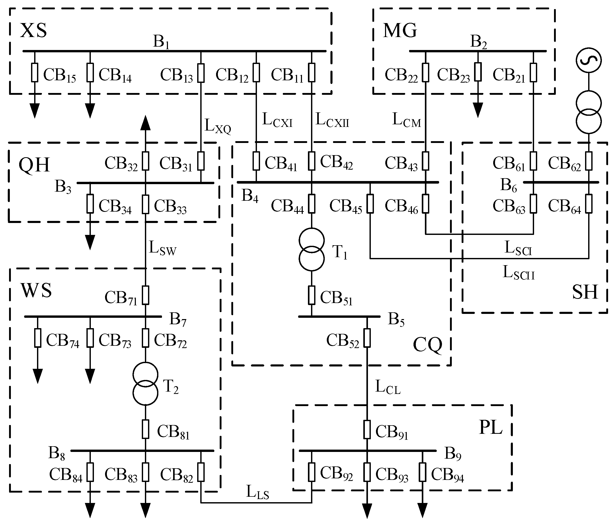
4.2. Actual Case Analysis
4.2.1. Case 1
- CBS = {CB71} can be obtained from the alarm message. Traverse CBS and search for suspected faulty components. There are a subset COM71 = {LSW, LXQ, B3, B7}, and a total set COMS = {LSW, LXQ, B3, B7}.
- LSW is selected for fault diagnosis. The , , , and of the fault diagnosis model for the CB71and CB33 subnets are as follows.
- The diagnosis results for the CB71 subnet are αp10(11) = 0.9873 and Tp10(11) = [−40, −10]. The diagnosis results of the CB33 subnet are αp10(12) = 0.5567 and Tp10(12) = [−35, −5]. The diagnosis results of LSW are α(1) = 0.7915 and T(1) = [−35, −10], and its measured value η(1) = 0.8540, which is greater than 0.6. Thus, T1213 is a faulty component.
- Similarly, the measured values of LXQ, B3 and B7 are 0.2363, 0.14, and 0.2085, respectively, and they are non-faulty components.
4.2.2. Case 2
- CBS = {CB51, CB91} can be obtained from the alarm message. Traverse CBS and search for suspected faulty components. There are a subset COM51 = {B5, T1, B4, LCXI, BCXII, LCM, LSCI, LSCII}, a subset COM91 = {B9, LCL, B5, T1}, and a total set COMS = {B5, T1}.
- B5 is selected for fault diagnosis. The , , , and of the fault diagnosis model for the CB51 and CB52 subnets are as follows.
- The diagnosis results for the CB51 subnet are αp10(11) = 0.9873 and Tp10(11) = [−40, −10]. The diagnosis results of the CB52 subnet are αp10(12) = 0.5567 and Tp10(12) = [−15, 15]. The diagnosis results of B5 are α(1) = 0.7915 and T(1) = [−15, −10], and its measured value η(1) = 0.8540, which is greater than 0.6. Thus, B5 is a faulty component.
- Similarly, the measured value of T1 is 0.2363, and T1 is a non-faulty component.
4.2.3. Case 3
- CBS = {CB44, CB51} can be obtained from the alarm message. Traverse CBS and search for suspected faulty components. There is a subset COM44 = {B4, T1, B5, LCL}, a subset COM51 = {B5, T1, LCXI, B4, LCXII, LCM, LSCI, LSCII}, and a total set COMS = {T1, B4, B5}.
- T1 is selected for fault diagnosis. The , , , and of the fault diagnosis model for the CB44 and CB51 subnets are as follows.
- The diagnosis results for the CB44 subnet are αp10(11) = 0.8797 and Tp10(11) = [−40, −10]. The diagnosis results of the CB51 subnet are αp10(12) = 0.8795 and Tp10(12) = [−40, 40]. The diagnosis results of T1213 are α(1) = 0.8795 and T(1) = [−40, −10], and its measured value η(1) = 0.9156, which is greater than 0.6. Thus, T1 is a faulty component.
- Similarly, the measured values of B4 and B5 are 0.1857 and 0.1881, respectively, and they are non-faulty components.
4.3. Comparison Analysis with Other Methods
4.3.1. Case Result Comparisons
4.3.2. Performance Comparison
5. Conclusions
Author Contributions
Funding
Institutional Review Board Statement
Informed Consent Statement
Data Availability Statement
Conflicts of Interest
References
- Kaluder, S.; Fekete, K.; Jozsa, L.; Klaic, Z. Fault Diagnosis and Identification in the Distribution Network Using the Fuzzy Expert System. Eksploat. I Niezawodn.-Maint. Reliab. 2018, 20, 621–629. [Google Scholar] [CrossRef]
- Perez, R.; Inga, E.; Aguila, A.; Vasquez, C.; Lima, L.; Viloria, A.; Henry, M.-A. Fault Diagnosis on Electrical Distribution Systems Based on Fuzzy Logic. In Proceedings of the 9th International Conference on Swarm Intelligence (ICSI), Shanghai, China, 17–22 July 2018; pp. 174–185. [Google Scholar]
- Xiong, G.; Shi, D.; Zhang, J.; Zhang, Y. A binary coded brain storm optimization for fault section diagnosis of power systems. Electr. Power Syst. Res. 2018, 163, 441–451. [Google Scholar] [CrossRef]
- Wang, S.; Zhao, D.; Yuan, J.; Li, H.; Gao, Y. Application of NSGA-II Algorithm for fault diagnosis in power system. Electr. Power Syst. Res. 2019, 175, 105893. [Google Scholar] [CrossRef]
- Wang, S.-P.; Zhao, D.-M. A Hierarchical Power Grid Fault Diagnosis Method Using Multi-Source Information. IEEE Trans. Smart Grid 2020, 11, 2067–2079. [Google Scholar] [CrossRef]
- Yang, Q.; Le Blond, S.; Aggarwal, R.; Wang, Y.; Li, J. New ANN method for multi-terminal HVDC protection relaying. Electr. Power Syst. Res. 2017, 148, 192–201. [Google Scholar] [CrossRef]
- Han, J.; Miao, S.; Li, Y.; Yang, W.; Yin, H. Faulted-Phase classification for transmission lines using gradient similarity visualization and cross-domain adaption-based convolutional neural network. Electr. Power Syst. Res. 2021, 191, 106876. [Google Scholar] [CrossRef]
- Han, Y.; Tong, X. Power System Fault Diagnosis Based on Dynamic Reasoning Chain. Power Syst. Technol. 2017, 41, 1315–1323. [Google Scholar]
- Lin, S.; Chen, X.; Wang, Q. Fault diagnosis model based on Bayesian network considering information uncertainty and its application in traction power supply system. IEEJ Trans. Electr. Electron. Eng. 2018, 13, 671–680. [Google Scholar] [CrossRef]
- Zhang, Y.; Zhang, Y.; Wen, F.; Chung, C.Y.; Tseng, C.-L.; Zhang, X.; Zeng, F.; Yuan, Y. A fuzzy Petri net based approach for fault diagnosis in power systems considering temporal constraints. Int. J. Electr. Power Energy Syst. 2016, 78, 215–224. [Google Scholar] [CrossRef]
- Kiaei, I.; Lotfifard, S. Fault Section Identification in Smart Distribution Systems Using Multi-Source Data Based on Fuzzy Petri Nets. IEEE Trans. Smart Grid 2020, 11, 74–83. [Google Scholar] [CrossRef]
- Yuan, C.; Liao, Y.; Kong, L.; Xiao, H. Fault diagnosis method of distribution network based on time sequence hierarchical fuzzy petri nets. Electr. Power Syst. Res. 2021, 191, 106870. [Google Scholar] [CrossRef]
- Zhang, X.; Yue, S.; Zha, X. Method of power grid fault diagnosis using intuitionistic fuzzy Petri nets. IET Gener. Transm. Distrib. 2018, 12, 295–302. [Google Scholar] [CrossRef]
- Wang, J.; Peng, H.; Tu, M.; Perez-Jimenez, J.M.; Shi, P. A Fault Diagnosis Method of Power Systems Based on an Improved Adaptive Fuzzy Spiking Neural P Systems and PSO Algorithms. Chin. J. Electron. 2016, 25, 320–327. [Google Scholar] [CrossRef]
- Rong, H.; Yi, K.; Zhang, G.; Dong, J.; Paul, P.; Huang, Z. Automatic Implementation of Fuzzy Reasoning Spiking Neural P Systems for Diagnosing Faults in Complex Power Systems. Complexity 2019, 2019, 2635714. [Google Scholar] [CrossRef]
- Wang, T.; Zhang, G.; Zhao, J.; He, Z.; Wang, J.; Perez-Jimenez, M.J. Fault Diagnosis of Electric Power Systems Based on Fuzzy Reasoning Spiking Neural P Systems. IEEE Trans. Power Syst. 2015, 30, 1182–1194. [Google Scholar] [CrossRef]
- Peng, H.; Wang, J.; Ming, J.; Shi, P.; Perez-Jimenez, M.J.; Yu, W.; Tao, C. Fault Diagnosis of Power Systems Using Intuitionistic Fuzzy Spiking Neural P Systems. IEEE Trans. Smart Grid 2018, 9, 4777–4784. [Google Scholar] [CrossRef]
- Wang, J.; Peng, H.; Yu, W.; Ming, J.; Perez-Jimenez, M.J.; Tao, C.; Huang, X. Interval-valued fuzzy spiking neural P systems for fault diagnosis of power transmission networks. Eng. Appl. Artif. Intell. 2019, 82, 102–109. [Google Scholar] [CrossRef]
- Liu, W.; Wang, T.; Zang, T.; Huang, Z.; Wang, J.; Huang, T.; Wei, X.; Li, C. A Fault Diagnosis Method for Power Transmission Networks Based on Spiking Neural P Systems with Self-Updating Rules considering Biological Apoptosis Mechanism. Complexity 2020, 2020, 2462647. [Google Scholar] [CrossRef]
- Huang, K.; Wang, T.; He, Y.; Zhang, G.; Pérez-Jiménez, M.J. Temporal fuzzy reasoning spiking neural P systems with real numbers for power system fault diagnosis. J. Comput. Theor. Nanosci. 2016, 13, 3804–3814. [Google Scholar] [CrossRef]
- Wang, T.; Wei, X.; Wang, J.; Huang, T.; Peng, H.; Song, X.; Valencia Cabrera, L.; Perez-Jimenez, M.J. A weighted corrective fuzzy reasoning spiking neural P system for fault diagnosis in power systems with variable topologies. Eng. Appl. Artif. Intell. 2020, 92, 103680. [Google Scholar] [CrossRef]
- Lin, D. A fault diagnosis method for power grid based on time sequential spiking neural P systems. New Tech. New Products China. 2022, 2, 1–7. [Google Scholar]
- Xiong, G.; Shi, D.; Zhu, L.; Duan, X. A New Approach to Fault Diagnosis of Power Systems Using Fuzzy Reasoning Spiking Neural P Systems. Math. Probl. Eng. 2013, 2013, 815352. [Google Scholar] [CrossRef]
- Guo, W.; Wen, F.; Ledwich, G.; Liao, Z.; He, X.; Huang, J. A new analytic approach for power system fault diagnosis employing the temporal information of alarm messages. Int. J. Electr. Power Energy Syst. 2012, 43, 1204–1212. [Google Scholar] [CrossRef]


| Components | Line | Bus | Transformer | |
|---|---|---|---|---|
| Main | PR | 0.9913 | 0.8564 | 0.7756 |
| CB | 0.9833 | 0.9833 | 0.9833 | |
| Near backup | PR | 0.80 | 0 | 0.75 |
| CB | 0.85 | 0 | 0.8 | |
| Remote backup | PR | 0.70 | 0.70 | 0.70 |
| CB | 0.75 | 0.75 | 0.75 | |
| No. | Fault Descriptions | Brief Descriptions | Suspected Faulty Components | Spike Values | Time-Point Constraints | Measured Values | Faulty Components |
|---|---|---|---|---|---|---|---|
| 4 | The fault occurs on B18, and the alarm message of CB0318 is missing. | Bp18(0), CB1817(29) | B18 | 0.7240 | [−40, −20] | 0.8068 | B18 |
| B17 | 0.2917 | 0.2042 | |||||
| L1718 | 0.3958 | 0.2771 | |||||
| L1727 | 0.2688 | 0.1881 | |||||
| L1617 | 0.2688 | 0.1881 | |||||
| 5 | A fault occurs on B18, CB1803 fails to trip, Lp0318s operates, and CB0318 trips. | Bp18(0), CB1718(29), Lp0318s(520), CB0318(540) | B18 | 0.8549 | [−20, −10] | 0.8757 | B18 |
| L1718 | 0.5625 | 0.3938 | |||||
| 6 | A fault occurs on B03, and the alarm on Bp03 is missing. | CB0302(29), CB0304(31), CB0318(32) | B03 | 0.5917 | [−48, −1] | 0.7142 | B03 |
| 7 | A fault occurs on B03, Bp03 fails to operate, and remote backup PRs operate. | Lp1803s(0), Lp0403s(2), Lp0203s(6), CB1803(32), CB0403(35), CB0203(36) | B03 | 0.725 | [−534, −510] | 0.8075 | B03 |
| L0203 | 0.6583 | 0.4608 | |||||
| L0304 | 0.6583 | 0.4608 | |||||
| L0318 | 0.6583 | 0.4608 | |||||
| 8 | A fault occurs on L0318, Lp1803m fails to operate, and Lp1803p operates, but the timestamp of Lp1803p is incorrect. | Lp0318m(0), CB0318(30), Lp1803p(200), CB1803(325) | L0318 | 0.9062 | [−40, −5] | 0.9343 | L0318 |
| 9 | A fault occurs on L0318, CB1803 fails to trip, and the alarm message of Lp0318m is missing. | Lp1803m(0), CB0318(25), Lp1718s(500), CB1718(515) | L0318 | 0.6583 | [−40, −10] | 0.7608 | L0318 |
| L1718 | 0.5333 | 0.3733 | |||||
| B18 | 0.6 | 0.42 | |||||
| 10 | A fault occurs on L0318, CB1803 fails to trip, and the alarm message of CB0318 is missing. | Lp0318m(0), Lp1803m(5), Lp1718s(500), CB1718(515) | L0318 | 0.6603 | [−35, −10] | 0.7622 | L0318 |
| L1718 | 0.3958 | 0.2771 | |||||
| B18 | 0.4625 | 0.3238 | |||||
| B17 | 0.3958 | 0.2771 | |||||
| 11 | A fault occurs on T1213 and the alarm message of CB1312 is missing. | Tp1213m(0), CB1213(5) | T1213 | 0.6836 | [−40, −10] | 0.7785 | T1213 |
| B12 | 0.3958 | 0.2771 | |||||
| B13 | 0.2917 | 0.2042 | |||||
| L1314 | 0.2688 | 0.1881 | |||||
| L1013 | 0.2688 | 0.1881 | |||||
| 12 | A fault occurs on T1213, CB1803 fails to trip, Lp1413 and Lp1013s operate, and CB1413 and CB1013 trip. | Tp1213m(0), CB1213(32), Lp1413s(525), Lp1013s(530), CB1413(540), CB1013(545) | T1213 | 0.8224 | [−15, −10] | 0.8757 | T1213 |
| B13 | 0.475 | 0.3325 | |||||
| L1314 | 0.5333 | 0.3733 | |||||
| L1013 | 0.5333 | 0.3733 | |||||
| 13 | A fault occurs on L0318, the alarm message of CB0318 is missing. A fault occurs on L1718. | Lp0318m(0), Lp1803m(5), CB1803(35), Lp1817m(120), Lp1718m(128), CB1817(145), CB1718(153) | L0318 | 0.7915 | [−35, −10] | 0.8540 | L0318 L1718 |
| L1718 | 0.9873 | [88, 110] | 0.9911 | ||||
| B17 | 0.3306 | 0.2314 | |||||
| B18 | 0.5917 | 0.4142 | |||||
| 14 | A fault occurs on L0318, and CB1803 fails to trip. A fault occurs on B17. | Lp1803m(0), Lp0318m(2), CB0318(30), Lp1718s(520), CB1718(541), Bp17(100), CB1727(135), CB1716(140), | L0318 | 0.8562 | [−20, 10] | 0.8993 | L0318 B17 |
| L1718 | 0.5333 | 0.3733 | |||||
| B17 | 0.9199 | [60, 80] | 0.9493 | ||||
| B18 | 0.6 | 0.42 | |||||
| 15 | A fault occurs on B03, the alarm message of CB0318 is missing. A fault occurs on B03, but the timestamp of CB1415 is incorrect. | Bp03(0), CB0302(29), CB0304(31), Bp14(250), CB1404(275), CB1415(284), CB1413(385) | B03 | 0.8549 | [−27, −10] | 0.8984 | B03 B14 |
| B14 | 0.9199 | [210, 240] | 0.9493 | ||||
| 16 | A fault occurs on B18, Bp18 fails to operate, and remote backup PRs operate. A fault occurs on T1213, and the alarm on Bp11 is missing; a fault occurs on L0204. | Lp0318s(0), Lp1718s(5), CB0318(32), CB1718(35) CB1312(50), CB1213(60) | B18 | 0.725 | [−534, −510] | 0.8075 | B18 T1213 |
| L0318 | 0.6583 | 0.4608 | |||||
| L1718 | 0.6583 | 0.4608 | |||||
| T1213 | 0.5917 | [−20, 20] | 0.7142 | ||||
| B12 | 0.3958 | 0.2771 | |||||
| B13 | 0.3306 | 0.2314 |
| No. | Suspected Faulty Components | Fault Diagnosis Results | Faulty Components | ||||||||
|---|---|---|---|---|---|---|---|---|---|---|---|
| [16,21,22] | This Study | [13] | [23] | [17] | [18] | [20] | [21] | [22] | This Study | ||
| 1 | B18 | B18 | B18 | B18 | B18 | B18 | B18 | B18 | B18 | B18 | B18 |
| 2 | L0318, L1718, B18 | L0318, L1718, B18 | L0318, B18 | L0318 | L0318, B18 | L0318, B18 | L0318 | L0318, B18 | L0318 | L0318 | L0318 |
| 3 | - | T1213, B12, B13, L1314, L1013 | T1213 | - | T1213 | - | - | T1213 | - | T1213 | T1213 |
| 4 | - | B18, B17, L1718, L1727, L1617 | B18 | - | B18 | B18 | B18 | B18 | B18 | B18 | B18 |
| 5 | L0318, B03 | B18, L1718 | B18 | B18 | B18 | B18 | B18 | B18 | B18 | B18 | B18 |
| 6 | B03 | B03 | B03 | - | - | - | - | - | B03 | B03 | B03 |
| 7 | B03, L0203, L0304, L0318 | B03, L0203, L0304, L0318 | B03, L0203, L0304, L0318 | B03 | B03, L0203, L0304, L0318 | B03, L0203, L0304, L0318 | B03 | B03 | B03 | B03 | B03 |
| 8 | L0318 | L0318 | L0318 | L0318 | L0318 | L0318 | L0318 | - | L0318 | L0318 | L0318 |
| 9 | L0318, L1718, B18 | L0318, L1718, B18 | L0318, B18 | - | L0318, B18 | L0318, B18 | - | B18 | L0318 | L0318 | L0318 |
| 10 | - | L0318, L1718, B18, B17 | L0318, B18, L1718 | - | L0318, B18 | L0318, B18 | - | B18 | L0318 | L0318 | L0318 |
| 11 | - | T1213, B12, B13, L1314, L1013 | T1213 | - | T1213 | - | - | T1213 | - | T1213 | T1213 |
| 12 | T1213, B13, L1314, L1013 | T1213, B13, L1314, L1013 | T1213, B13, L1314, L1013 | - | T1213, B13, L1314, L1013 | B13, L1314, L1013 | - | T1213 | - | T1213 | T1213 |
| 13 | B18, L1718 | L0318, L1718, B17, B18 | L1718 | L1718 | L1718 | L1718 | L1718 | L1718 | L1718 | L0318, L1718 | L0318, L1718 |
| 14 | L0318, L1718, B17, B18 | L0318, L1718, B17, B18 | L0318, B17, B18 | L0318, B17 | L0318, B17 | L0318, B17 | L0318, B17 | L0318, B17 | L0318, B17 | L0318, B17 | L0318, B17 |
| 15 | B14 | B03, B14 | B14 | B14 | B14 | B14 | B14 | B14 | B14 | B03, B14 | B03, B14 |
| 16 | B18, L0318, L1718, T1213 | B18, L0318, L1718, T1213, B12, B13 | B18, L0318, L1718, T1213 | B18 | B18, L0318, L1718 | B18, L0318, L1718 | B18 | B18 | B18 | B18, T1213 | B18, T1213 |
| [13] | [23] | [17] | [18] | [20] | [21] | [22] | This Study | |
|---|---|---|---|---|---|---|---|---|
| Consideration of temporal features | No | No | No | No | Yes | Yes | Yes | Yes |
| Consideration of neighboring components configured with the backup protection | No | Yes | No | No | Yes | Yes | Yes | Yes |
| Consideration of incorrect operations of the PRs and CBs | Yes | Yes | Yes | Yes | Yes | Yes | Yes | Yes |
| Consideration of missing alarms of the boundary CBs | No | No | No | No | No | No | No | Yes |
| Consideration of the uncertainty of alarm messages | Yes | No | Not considering the main protection of the bus and transformer | Not considering the main protection of the bus and transformer | Not considering the main protection of the bus and transformer | Not considering the main protection of the bus and transformer | Yes | Yes |
| Consideration of timing errors | No | No | Yes | No | Yes | No | Yes | No |
| Accuracy and fault tolerance | General | Poor | General | General | Good | Good | Excellent | Excellent |
| Method | Fault Diagnosis Models | Search Method for Suspected Faulty Components | Calculation Tasks | Calculation Methods and Calculation Amounts | Performance |
|---|---|---|---|---|---|
| This study | No need to build separate models No need to adjust diagnosis models for topology changes | Search for suspected faulty components configured the tripped CBs | Correlation reasoning between confidence degrees and temporal constraints | Matrix operation with a calculation amount of μν | Simple reasoning and calculation principles Strong generality and adaptability of the fault diagnosis model |
| [24] | Construction of the objective function based on the alarm message | Search the outage area to identify suspected faulty components | Fault hypothesis with the minimum loss value | Look-up table and optimization algorithm with a calculation amount of | Relatively slow convergence speed High calculation complexity |
| [10] | Individual construction of fault diagnosis models for suspected faulty components. Need for reconstruction of models based on topology changes for fault diagnosis. | Temporal matching of alarm messages Fuzzy reasoning of confidence degrees | Event correlation, look-up table, and matrix operation with a calculation amount of μ2ν | Independence of confidence reasoning and temporal reasoning processes High complexity in the alarm message association and temporal matching process | |
| [20] | Temporal matching and classification of alarm messages Fuzzy reasoning of confidence degrees | Event correlation, look-up table, and matrix operation with a calculation amount of 2μν | |||
| [21] | Temporal matching of alarm messages Fuzzy reasoning of confidence degrees | Event correlation, look-up table, and matrix operation with a calculation amount of 2μν | |||
| [22] | Correlation reasoning between confidence degrees and temporal constraints | Matrix operation with a calculation amount of μν | Relatively complex reasoning and calculation process in fault diagnosis High efficiency in diagnosis Lack of consideration for transformer fault diagnosis |
Disclaimer/Publisher’s Note: The statements, opinions and data contained in all publications are solely those of the individual author(s) and contributor(s) and not of MDPI and/or the editor(s). MDPI and/or the editor(s) disclaim responsibility for any injury to people or property resulting from any ideas, methods, instructions or products referred to in the content. |
© 2024 by the authors. Licensee MDPI, Basel, Switzerland. This article is an open access article distributed under the terms and conditions of the Creative Commons Attribution (CC BY) license (https://creativecommons.org/licenses/by/4.0/).
Share and Cite
Shao, N.; Chen, Q.; Xie, D.; Sun, Y.; Yu, C. Improved Temporal Fuzzy Reasoning Spiking Neural P Systems for Power System Fault Diagnosis. Appl. Sci. 2024, 14, 1753. https://doi.org/10.3390/app14051753
Shao N, Chen Q, Xie D, Sun Y, Yu C. Improved Temporal Fuzzy Reasoning Spiking Neural P Systems for Power System Fault Diagnosis. Applied Sciences. 2024; 14(5):1753. https://doi.org/10.3390/app14051753
Chicago/Turabian StyleShao, Ning, Qing Chen, Dan Xie, Ye Sun, and Chengao Yu. 2024. "Improved Temporal Fuzzy Reasoning Spiking Neural P Systems for Power System Fault Diagnosis" Applied Sciences 14, no. 5: 1753. https://doi.org/10.3390/app14051753
APA StyleShao, N., Chen, Q., Xie, D., Sun, Y., & Yu, C. (2024). Improved Temporal Fuzzy Reasoning Spiking Neural P Systems for Power System Fault Diagnosis. Applied Sciences, 14(5), 1753. https://doi.org/10.3390/app14051753