Electro-Magnetic and Stress Analysis of a −400 T²/m High-Field Gradient Magnet with a Room-Temperature Bore Size of 200 mm

Featured Application

The superconducting magnet designed in this article will be used as an experimental device to provide various gravity field environments at different levels for Ga_1−xIn_xSb crystal growth research topics.

Abstract

High-field-strength gradient superconducting magnets have been widely used in many fields. With advancements in technology, the demand for large-aperture magnets is gradually increasing, but there is relatively little research on the design and stress–strain of large-aperture gradient magnets. This article presents the design and analysis of a superconducting magnet characterized by a high field strength of 10 T, a strong gradient of −400 T²/m, and a large room-temperature bore of 200 mm. The aim of this project is to establish an experimental setup for the growth of Ga_1−xIn_xSb crystals. The study starts with an overview of the development process and applied research related to strong-gradient magnets. The study employs a magneto–electric force coupling method based on generalized stretching to theoretically optimize the gradient coil pre-stress parameters through orthogonalization parameter scanning. In addition, an analysis of the stress distribution in both the magnet coil and the mandrel is carried out. The results indicate that the stress and strain values for both the gradient coils and the frame are within the allowable range of their respective materials. The magnets can be designed to operate stably in theory. This article may provide a reference for designers in related fields in optimizing the design and stress–strain analysis of large, strong-gradient magnets.

1. Introduction

The abbreviations and acronyms mentioned in this article are presented in

Table 1. The abbreviations and acronyms mentioned in this article.

Serial Number	Abbreviations and Acronyms	Original Text before Abbreviation
1	JASTEC	Japan Superconductor Technology, Inc. (Kobe, Japan)
2	JMTA-16T50MF	Large-gradient high-field superconducting magnet with a central magnetic field of 16 T and a room-temperature bore of 50 mm
3	LH15T40	Large-gradient high-field superconducting magnet with a central magnetic field of 15 T and a room-temperature bore of 40 mm
4	WM4	Large-gradient high-field superconducting magnet in the Chinese High Magnetic Field Laboratory (Hefei, China)
5	LG-HMF	Large-gradient high magnetic field
6	S-HGMS	Superconducting high-gradient magnetic separation
7	HG-TFM	High-gradient trapped-field magnet

.

Superconducting magnets with high-field-strength gradients are widely used in various domains. A typical manufacturer of such superconducting magnets is JASTEC (Kobe, Japan). JASTEC [1] has developed and manufactured JMTA-16T50MF superconducting magnets with LG-HMF capabilities. These magnets are particularly suitable for simulating stable microgravity and supergravity through the application of gradient magnetic fields. Several researchers have used this device for research projects related to protein crystal growth [2,3,4,5,6]. The magnet has a maximum magnetic field strength of 16.12 T, with magnetic field gradients extending up to −1500 T²/m. However, a notable drawback of this superconducting magnet is its dependency on a continuous supply of liquid helium and liquid nitrogen during operation [7].

JASTEC also designs and manufactures another magnet: the LH15T40. The magnet can generate magnetic field gradients up to −150 T/m and operates normally without current. Yin et al. [8] successfully used this magnet to obtain a quasi-microgravity environment. Later, Wakayama et al. [9] used the same magnet to simulate the microgravity environment in space and studied the crystallization of orthogonal lysozyme under pseudo-microgravity conditions.

In 2020, Qingping Tao [10] and others used the WM4 superconducting magnet manufactured by the Chinese Academy of Sciences to detect the magnetic properties of non-fixed, non-dehydrated living cells and cell components. The characteristic of this magnet is that it can generate extremely high field strengths, but because of its small aperture, the applicable sample diameter and the use of test instruments are limited. Combined with Er-Kai Yan’s [7] introduction to gradient magnets, the advantages and disadvantages of various high-field-strength gradient magnets are summarized in

Table 2. The advantages and disadvantages of various high-field-strength gradient magnets.

Magnets	Room-Temperature Bore Size	Center Field Strength	Advantages and Disadvantages
JMTA-16T50MF	50 mm	16.12 T	The magnetic field gradient value is high and the operation is stable, but it requires a continuous supply of liquid helium and the aperture is small at room temperature.
LH15T40	40 mm	15 T	The magnet can generate magnetic field gradients up to 150 T/m and operates normally without current.
WM4	32 mm	23.5 T	This magnet can reach extremely high field strengths, and both the gradient value and the field strength value can be adjusted. However, the use space is limited, and it is not highly adaptable to large-sized experimental materials.

.

As science and technology continue to advance, high-gradient magnets have found diverse applications. Li Yongkui [11] used superconducting high-gradient magnetic separation (S-HGMS) to extract quartz from sea sand. Weak magnetic particles in sea sand are selectively converted into tailings, and quartz pre-enrichment is achieved under high magnetic field intensity. Xie Yucai [12] employed a miniature triple-coil multi-pollutant detection sensor based on high-gradient magnetic fields to detect ferromagnetic particles, non-magnetic particles, and moisture. It shows that the micro three-coil multi-pollutant detection sensor based on high-gradient magnetic field can achieve high-precision detection of ferromagnetic particles, non-ferromagnetic particles, and moisture.

In 2021, Takahashi Keita et al. [13,14] introduced a conceptual study on the design of a high-gradient trapped-field magnet (HG-TFM) with the objective of creating quasi-zero-gravity conditions on Earth. Within their project, numerical simulations were employed to analyze the electromagnetic stresses associated with this magnet. Similarly, the team led by D. N. Diev [15] analyzed and computed the electromagnetic stress within the electromagnetic system of their designed magnetic separator, accompanied by preliminary testing activities.

From the above cases, two pieces of information can be found:

• The main method of researchers is to directly utilize gradient magnets as experimental tools, while paying limited attention to the design process and stress analysis of the high-gradient magnet itself.
• Although existing high-gradient magnets can achieve higher gradient values, their room-temperature pore sizes are usually small, which makes them insufficient to meet the changing needs of technological advancement.

During the operation of the magnet coil, the electromagnetic stress generated by the Lorentz force will become an inducing factor for the displacement of the superconducting wire in the coil winding. When the electromagnetic stress is too large, it will also cause the magnet to lose its superconductivity. Most importantly, as the center-field strength of the magnet increases, the effect of electromagnetic stress in the magnet windings becomes more severe. Given that these types of gradient magnets typically exhibit a substantial central magnetic field strength and a high magnetic field gradient, the operation of the magnets can result in the generation of significant electromagnetic stress in the superconducting coils and supporting structures [16].

The commonly used methods for calculating electromagnetic stress include the analytical method and the finite element method. For gradient superconducting magnets, due to their complex magnetic field distribution and uneven stress distribution, it is generally difficult to handle these problems using the analytical method. In particular, as the design diameter of the magnet becomes larger, the design difficulty of the magnet gradually increases. For large-diameter high-field-intensity gradient magnets, the stress condition of the mechanical system is severe. Through finite element analysis, one can attain the results that have been shown in the aforementioned literature, as well as understanding the stress distribution state inside the magnet coil; you can also calculate the stress and strain conditions of mechanical systems beyond those of the magnet coil, through multi-field coupling analysis. On this basis, you can quickly optimize the parameters of the magnet. In this study, we will analyze the electromagnetic stress–strain values of a high-field-gradient magnet with a gradient of −400 T²/m, designed by our laboratory, using the finite element method. The objective is to offer design insights and methodological references for researchers engaged in the study of strong-gradient magnets.

2. High-Field-Gradient Magnet Structures

2.1. Electromagnetic Parameters of the Gradient Magnet

Table 3. Design prerequisites for the gradient magnet.

Central Magnetic Field	Magnetic Field Gradient Extreme Value (Absolute Value)	Room-Temperature Diameter	System Outer Diameter	Cooling Method
10 T	400 T2/m	200 mm	≤1100 mm	Zero-liquid helium evaporation refrigeration system

lists the basic design prerequisites for gradient magnets. The original standard required that the central magnetic field strength should exceed 10 T to effectively control crystal growth behavior in high magnetic fields. Secondly, in order to control the simulated gravity, it is necessary to calculate the distribution and extreme point of the product of the magnetic field and the field gradient on the z-axis, which is expressed in its functional form as B (dB/dz).

In order to form a 0–2 g gravity simulation field, the second standard stipulates that the maximum gradient absolute value along the central axis should reach 400 T²/m. The remaining indicators are determined by experimental parameters. As new crystal growth research continues to unfold, new requirements are put forward for the size of the operating space.

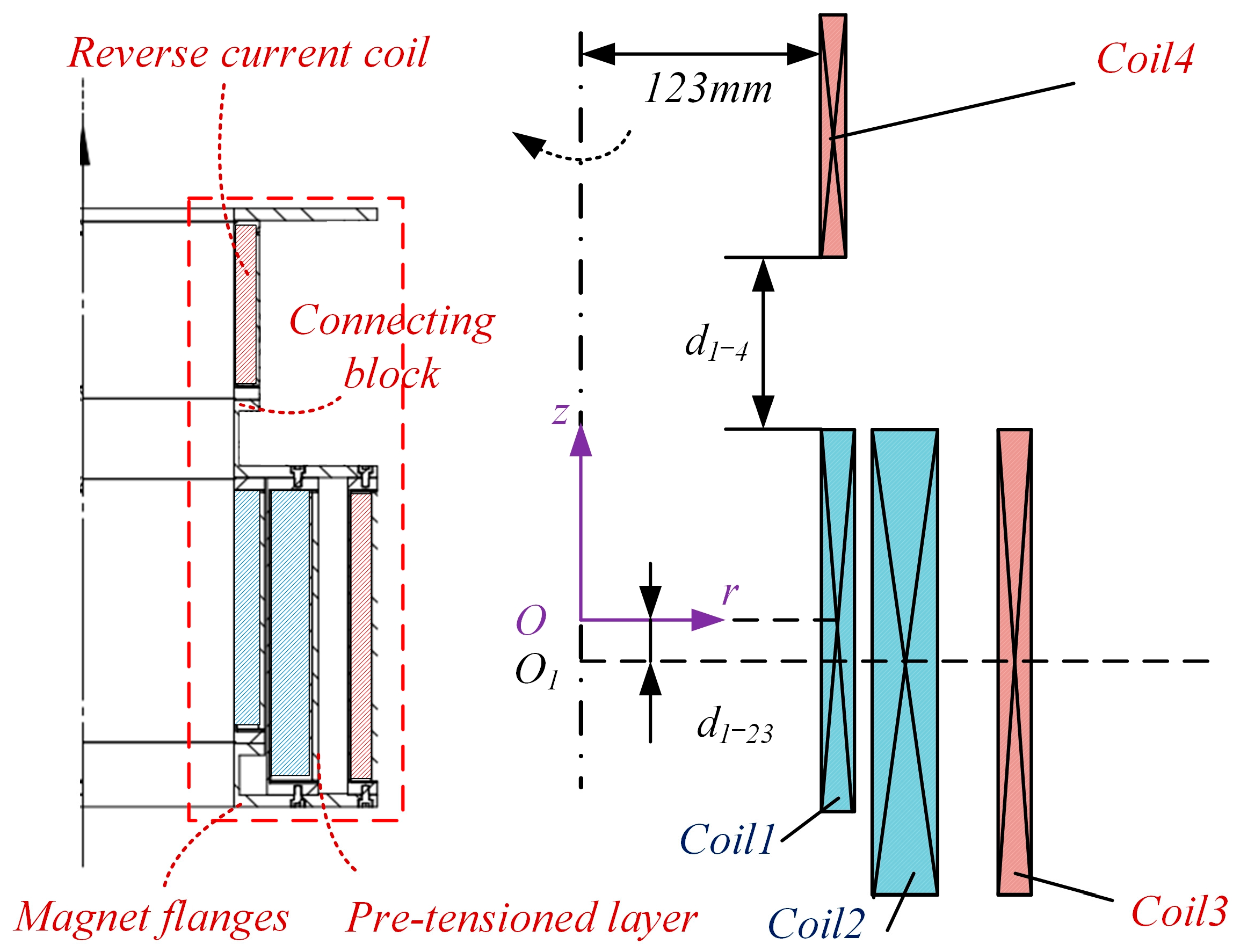
As shown in Figure 1, the magnet coil is intended to be wound using an odd–even layer winding technique. To enhance the magnetic field gradient and reduce the external diameter of the magnet, an additional coil with reverse current is added in the longitudinal direction.

The magnet utilizes a zero-liquid helium evaporation system for cooling. Given the necessity for a room-temperature aperture of ≥200 mm, the installation of a cold screen and vacuum chamber is imperative between the room-temperature aperture and the inner diameter of the magnet. Drawing from practical experience, a minimum space of at least 20 mm needs to be allocated on one side. Therefore, the predetermined diameter for the magnet’s cooling aperture is set at 246 mm.

While satisfying the specified magnet parameters, the design places emphasis on the combined structure of the magnet coils, involving several variables: the axial distance (d_1–4) between coils 1 and 4; the deviation distance (d_1–23) between the centers of coil 1 and coils 2 and 3, between the single-layer turns, and between the layers of coil 4, as well as between the single-layer turns and the layers of coils 1, 2, and 3. According to engineering practice, one must note the distance between coils 1 and 2 and the gaps between coil 3, which consist of the thickness of the insulation layer, the thickness of the preload layer, and that of the coil gap. Under the premise of leaving a certain margin, these three types of thickness are all fixed values, and the space for optimization is small. Therefore, in this design, the gaps between coils 1, 2, and 3 do not need to be optimized. The ultimate goal of optimization is to minimize the cost of wire usage for the coils.

Table 4. Magnetic coil parameters.

Coil Number	Coil 1	Coil 2	Coil 3	Coil 4
Superconducting wire categories	HF Nb3Sn	ITER Nb3Sn	ITER PF NbTi	ITER PF NbTi
Wire diameter/mm	0.98	0.97	0.777	0.777
Inside diameter/mm	125.6	152.46	218.24	125.6
Outer diameter/mm	142.86	186.64	234.70	138.73
Bottom coordinate/mm	−99.64	−143.02	−142.70	189.64
Top coordinate/mm	99.64	99.64	99.64	316.35
Layers	20	40	24	19
Number of turns in odd-numbered layers	200	246	306	160
Peak field/T	13.04	9.972	6.139	5.680

presents the crucial electromagnetic parameters obtained after optimizing the magnet. The optimization iteration of electromagnetic field design is carried out step by step according to the following rules (Figure 2).

2.2. Structural Design of the Gradient Magnet

The gradient magnet comprises four coaxial but non-concentric coils, as illustrated in Figure 3. Coils 1–4 are wound around their respective mandrels, with each mandrel assembled as a unit through the articulating mandrel and articulating flange. Coils 1 and 2 are fabricated from HF Nb₃Sn/ITER Nb₃Sn, while coils 3 and 4 are composed of ITER PF NbTi. The sub-coils were wound on a 2 mm thick stainless steel (SS-316L) mandrel using a winding tension of 20 N. At 4.2K, the critical current of HF Nb₃Sn short wire samples exceeds 622 A at 12 T. For ITER Nb₃Sn, the critical current is 240 A at 12 T, and for ITER PF NbTi, the critical current is 190 A at 7 T. The wire parameters are detailed in

Table 5. Parameters of wires.

Parameters	HF Nb3Sn	ITER Nb3Sn	ITER PF NbTi
Dwire-insulated/mm	0.98	0.97	0.777
Dwire-bare/mm	0.85	0.818	0.727
Cu/non-Cu	0.46	1.0	2.3
RRR	>100	>100	>100
[email protected] K/A	≥622 @12T	≥240 @12T	≥190 @7T

.

Additionally, the quench–protection system is mounted on the top surface of the upper flange. This is because the diodes in the quench–protection system cannot withstand excessively strong magnetic fields. At the same time, in order to facilitate line connection, the quench–protection system should be as close as possible to the coil. In coils 1–4, the pre-tensioned layer is located outside the winding. The pre-tensioned layer material for Nb₃Sn coil is φ0.78 mm SS-316L stainless steel wire (Nanjing Futeng Electromechanical Equipment Co., Ltd., Nanjing, China), while for NbTi coil, it is a cross-section of 1.6 mm × 0.8 mm 6061 aluminum alloy tape (Wuxi Tongli Electrician Co., Ltd., Wuxi, China). Insulating layers are placed between the coil and the mandrel, as well as between the coil and the pre-tensioned layer, to preserve coil insulation.

2.3. Magnet Electromagnetic Field Simulation and Analysis

In this article, the finite element analysis software COMSOL Multiphysics 6.1 is employed for the simulation and analysis of the magnet’s electromagnetic scheme.

During the simulation process, the following settings need to be made to the model.

Model selection: This study selected a two-dimensional axisymmetric electromagnetic model, which was created from the solidworks 2021 version and imported into COMSOL; COMSOL was used to simplify the model. For the boundaries of the simulation domain, this study uses the infinite element function to add additional boundaries to the air domain. This processing can increase the speed of calculation and obtain more accurate results.

Grid processing: In order to simplify the calculation amount and improve the convergence speed, quadrilateral meshes are used for rectangular-shaped superconducting coils, and triangular meshes are used for irregularly shaped domains to ensure the continuity and continuity of the grids between each domain’s coupling. In particular, the grid in the air domain of this study is densified along the central axis, and the number of densification intervals is set to 500 to obtain an accurate simulation curve.

At an operating current of approximately 176.5 A, the magnet’s total energy storage is theoretically estimated to be around 1623.457 kJ, with an inductance value close to 104.23 H. The central (O₁) and peak magnetic fields of the magnet are 10.78 T and 13.04 T. Figure 4a illustrates the standard magnetic field concerning the radial coordinates of the magnet (z = 0), while Figure 4b illustrates the standard magnetic field concerning the axial coordinates of the magnet (r = 0). From Figure 4a, the radial standard magnetic field distribution can be obtained. When the magnetic induction line passes through the coil, the magnetic field will undergo a sudden change, and the corresponding point of change has been marked in the figure. At the same time, the cloud map in the lower left corner shows the distribution status of the magnetic field on the cross-section of the coil. From Figure 4b, the standard axial magnetic field distribution can be obtained. It can be seen that the magnetic field strength of the central axis of the magnet reaches a peak of 10.8 T in the middle of the three coils below. At the same time, the cloud map in the lower left corner shows the distribution of the magnetic field on the cross-section of the coils.

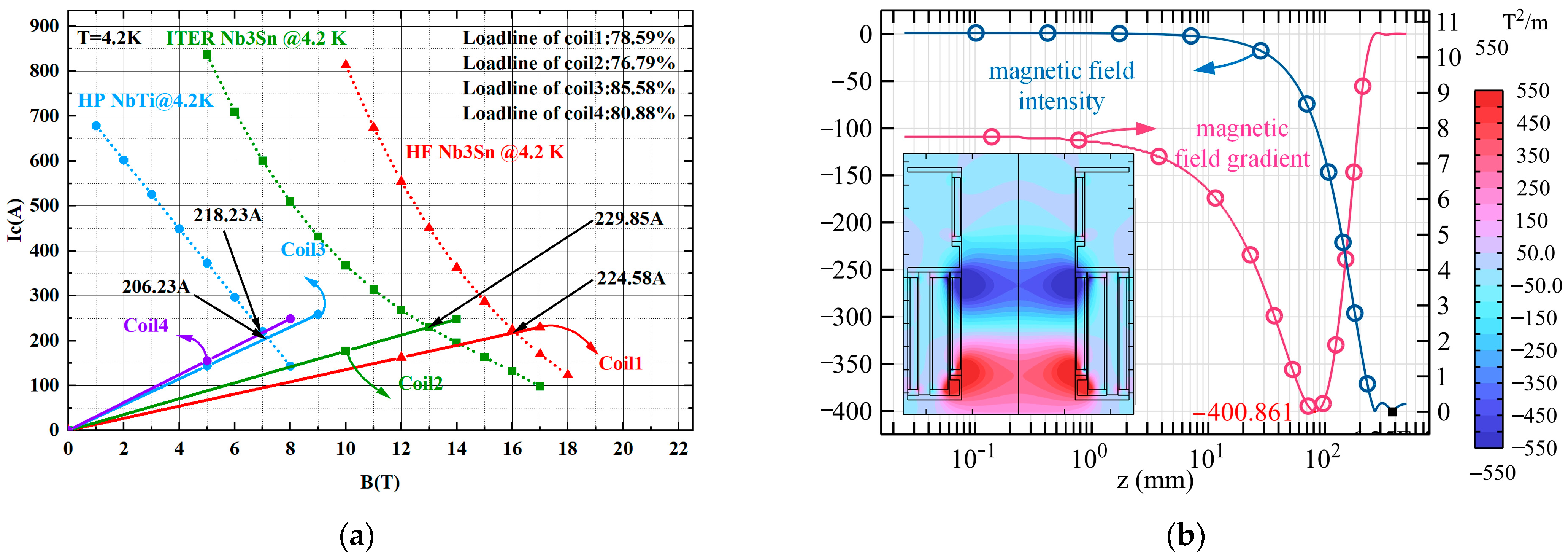
Based on the simulation results, load lines for the sub-coils can be plotted under the variation of the critical current with the magnetic field for the given superconducting short wire samples. The current utilization efficiency for coil 1 (defined as the ratio of the operating current to the critical current from the load line) is estimated to be 78.59%, for coil 2 it is estimated to be 76.79%, for coil 3 it is estimated to be 85.58%, and for coil 4 it is estimated to be 80.88%. These results are presented in Figure 5a. It can be seen from the figure that the current margin of the magnet coil is within an appropriate range and the risk of magnet quench is low.

The gradient value constitutes a critical design parameter for gradient magnets. To generate any horizontal simulated gravity field within the range of 0–2 g during the operation of superconducting magnets, the design requirements specify that the absolute value of the maximum gradient on the central axis of the magnet must exceed 400 T²/m. Figure 5b illustrates the gradient distribution along the center axis. In this figure, the gradient pole value of the magnetic field on the magnet’s central axis reaches approximately −400.861 T²/m, positioned at z = 81.19 mm, aligning with the established design criteria.

3. Theoretical Basis for Magnetic Coupled Field Simulation

3.1. Magnet-Averaged Finite Element Model

The adoption of a gradient magnet with a small superconducting wire diameter and a higher number of turns and layers result in a significant increase in the number of meshes and node density when using a detailed finite element model. This can lead to reduced convergence in model calculations. Therefore, an average finite element model [17,18,19] is introduced to treat the magnet equivalently. This approach considers different windings of superconducting wire or windings of the same type of superconducting wire with different duty cycles as independent domains for the solution. It is worth noting that, after vacuum impregnation or mixing with epoxy resin, the mechanical properties of the coil will no longer exhibit isotropy, and it is necessary to analyze its anisotropic parameters. According to this theory, each coil winding comprises a continuous anisotropic material that is equivalent to the winding. Consequently, the equivalent physical properties of the material must be determined using the composite law. When employing the average finite element model for simulation calculations, the impact of the original material’s discontinuity on the results is not considered.

As depicted in Figure 6, the average finite element model of the magnet utilizes the parity layer winding method for its winding. The main feature of this coil winding method is that the odd-numbered layers in the winding have one more turn than the even-numbered layers, and the wires in adjacent layers alternate with each other in the central axis direction, forming a regular hexagonal structure with a center angle of 60°. The smallest unit of the winding is a positive triangle, with superconducting wires constituting 90% and epoxy resin constituting 10%. Based on the above conclusion, the material of the superconducting coil is regarded as a composite material composed of epoxy resin and superconducting wire, which is equivalent to epoxy resin as the substrate, superconducting wire as fibers, with a fiber ratio of 0.9. The fibers are evenly distributed along the direction of the wire in the substrate.

For a circular superconducting wire with a rectangular cross-section, the equivalent Young’s modulus E₂, equivalent shear modulus G₁₂, and equivalent Poisson’s ratio v₁₂ are determined by the following empirical equations as follows [20]:

$$\frac{E_2}{E_m}=\frac{1+2\eta V_f}{1-\eta V_f}$$

(1)

$$\eta =\frac{\left(E_f/E_m\right)-1}{\left(E_f/E_m\right)+2}$$

(2)

$$\frac{G_{12}}{G_m}=\frac{1+\eta V_f}{1-\eta V_f}$$

(3)

$$\eta =\frac{\left(G_f/G_m\right)-1}{\left(G_f/G_m\right)+1}$$

(4)

$$v_{12}=v_f{V}_f+v_m{V}_m$$

(5)

The remaining variables in the formula are as follows: Young’s modulus of epoxy resin—E_m; Young’s modulus of superconductor—E_f; shear modulus of epoxy resin—G_m; shear modulus of superconductor—G_f; Poisson’s ratio of epoxy resin—v_m; Poisson’s ratio of superconductor—v_f; volume fraction of epoxy resin—V_m; volume fraction of superconductor—V_f.

The anisotropic physical property parameters of the equivalent material can be obtained, as shown in

Table 6. Equivalent physical properties of magnet materials (Western Superconducting Technology Co., Ltd., Xi’an, China).

Name	NbTi Coil	Nb3Sn Coil	316L
E-R/GPa	51.56	59.7	207
E-PHI/GPa	116	165	207
E-Z/GPa	51.56	59.7	207
v-RPHI	0.2964	0.354	0.29
v-PHIZ	0.296	0.36	0.29
v-RZ	0.2964	0.354	0.29
G-RPHI/GPa	16	17.6	-
G-PHIZ/GPa	44.75	60.6	-
G-RZ/GPa	16	17.6	-
ρ/kg/m3	6535	7048	7960

.

3.2. Magnetic Coupling Method Based on Generalized Stretching

Upon developing the average finite element model of the magnet, this study does not incorporate the electromagnetic–structural coupling node for electromagnetic stress analysis. This decision is based on the axisymmetric property of the gradient magnet, which enables the establishment of a two-dimensional rotating coordinate system O_r-z. The electromagnetic load is segmented into radial and circumferential components using the generalized stretching command, and these components are then applied to each node of the coil through the body load command to facilitate the calculation of electromagnetic and mechanical field coupling. Simultaneously, the program considers the magnet as a rotating body, simplifying the magnet model, and disregards the impact of coil insulation and coil outlet on the structural integrity of the magnet.

4. Magnet Stress Simulation and Analysis

4.1. Stress Analysis without Preload

When a magnet operates in a magnetic field, radial electromagnetic stresses are generated in the coil. For superconducting magnets, it is generally advised that the radial stress on each coil should be maintained at a relatively low level, with the theoretically optimal maximum value ideally being less than 0. In this particular magnet design, it is postulated that the electromagnetic stress in coils 1–3 could be potentially reduced by implementing pre-tensioned layer. As illustrated in Figure 7, without pre-tensioned layer to balance the electromagnetic force, the radial stress might reach approximately 26.9 MPa, and the peak equivalent stress on the mandrel could possibly attain 469 MPa, potentially surpassing the acceptable stress limit for 316L mandrel material by about 286 MPa at 4.2 K. Therefore, in addition to coil 4 remaining unchanged (the electromagnetic force of the reverse coil cannot be offset by the preload layer), applying an inward preload force on the outer surface of coils 1–3 is an ideal method of reducing system stress.

In gradient magnets, as the magnetic field distribution of the magnet is more irregular compared to that of a uniform field magnet, the coils are distributed asymmetrically in the mandrel, and after the mandrels are connected through the upper and lower end flanges, the preload force between different coils will be correlated to a certain extent. The principle is that the preload force triggers an overall deformation of the mandrel and has an influence on the stress values of the remaining coils. Excessive coil preload not only leads to increased stresses in the mandrel, but may also increase the radial stresses in the remaining coils. In the actual parameterization process, the reliability of the parameters cannot be determined by manual parameterization.

4.2. Optimization of Preload Parameters Based on Three-Factor Orthogonal Test

As mentioned in the previous subsection, manual tuning of the preload parameters in such gradient magnets poses challenges due to the response surface properties of the tuning parameters. To optimize these parameters for each coil, an experimental design based on three-factor orthogonal testing was implemented using the orthogonal parametric sweep function in COMSOL. The experimental design consisted of setting the highest stress value for coils 1–3 as the dependent variable, upper, and lower bounds on the design parameters and the number of levels, as detailed in

Table 7. Upper- and lower-parameter limits and levels of factors.

Name	Level	Minimum	Maximum
P1	21	40 [MPa]	50 [MPa]
P2	21	55 [MPa]	65 [MPa]
P3	11	5 [MPa]	10 [MPa]

.

We established a parameter scan in COMSOL, supplemented the manual parameterization, and conducted a parametric analysis of the preload forces P1, P2, and P3 of coils 1–3. Taking into account the actual working conditions of aluminum alloy strip winding (in large-size coil manufacturing, the preload force provided by the aluminum alloy strip is difficult to exceed 12 MPa), especially for the preload layer of coil 3, the upper limit of the preload force is set to 10 MPa.

The purpose of establishing a scan in this study is to quickly find the target interval value. Therefore, a between-parameters sensitivity analysis is not necessary. Since, in COMSOL, a single simulation time is very short, the weights of the preload forces P1, P2, and P3 can be set the same; they are quickly calculated by encrypting their respective intervals to simplify the process of parametric analysis. Using this method, 4851 sets of orthogonal parameter tests were generated, and the processing time was about 5 min.

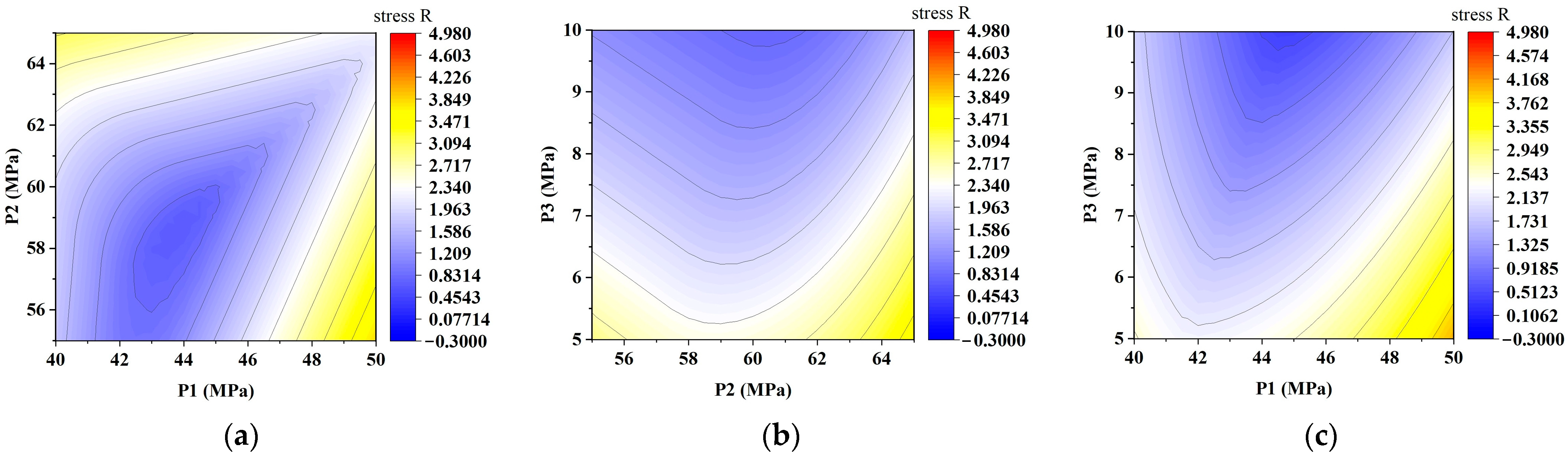
After solving, 4851 sets of maximum stress values of coils 1–3 can be obtained. After processing the data, the P1P2, P2P3, and P1P3 factor response surfaces are obtained, as shown in Figure 8. It can be seen from the figure that the response surface plot is tile-shaped. In the optimal solution area, 30 groups of solutions with negative stress peaks can be obtained, all of which are valid solutions. The contour line in the figure is the sum of the maximum radial stresses on the three coils. It can be seen that the effective solutions are distributed in the dark-blue area, and the darkest area is the theoretical optimal solution.

For all valid solutions, the maximum radial stress of the three coils can be close to 0. In order to reduce the difficulty of winding and the burden on the skeleton, this paper selects the parameters with the smallest total preload force in the solution area as the final design parameters, that is, P1 = 44.5 MPa, P2 = 57.5 MPa, and P3 = 9.5 MPa.

4.3. Magnet Coil and Mandrel Stress Results and Analysis

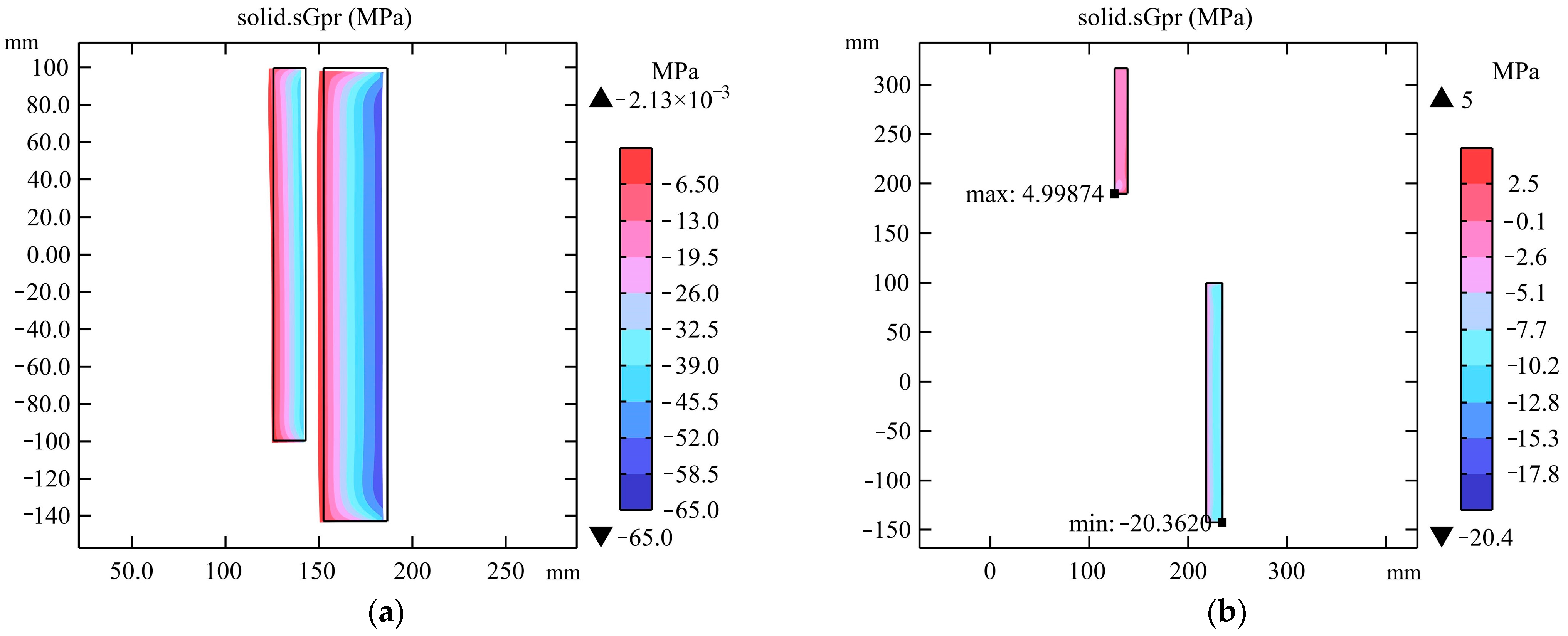
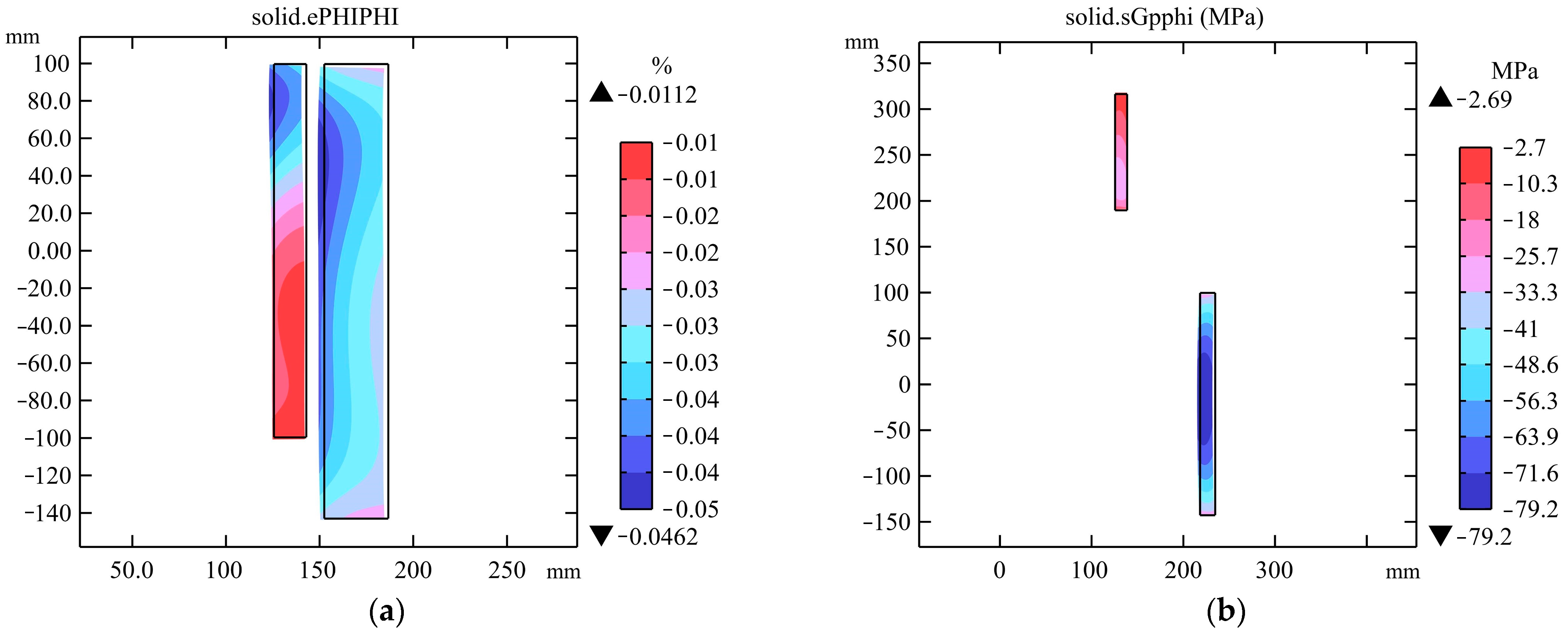
After determining the preload parameters using the method mentioned earlier, calculate the stress distribution of the magnet under the preload condition. Add generalized stretching modules in non-local coupling to the domain where each coil is located in COMSOL to obtain radial and circumferential stretching vectors. Afterwards, radial and circumferential Lorentz force loads were added to the coil domain in the electromagnetic module, and the radial and circumferential stress distributions for each coil were calculated as shown in Figure 9 and Figure 10. From Figure 9, it can be seen that the maximum radial stress of coils 1 and 3 is −2.13 × 10⁻³ MPa, close to 0. At the same time, the maximum radial stress of coil 4 is 5 MPa, which is still lower than the allowable shear stress of epoxy resin of 20 MPa.

Regarding circumferential stress, the maximum value for NbTi is found to be 79.2 MPa in Figure 10. This value is significantly lower than the allowable stress limit of 250 MPa at 4.2 K. In the case of Nb₃Sn coils, the engineering standard is often gauged by the ultimate yield strain, which is 0.2% of the material’s strength [19]. As illustrated in Figure 10, the maximum cyclic strain observed is 0.0462%, which falls well below the permissible strain value for the material at 4.2 K.

Figure 11 shows the radial stress changes of magnet coils 1–3 before and after adding preload force. It can be seen from the figure that after adding coil pre-tightening force, the peak radial stress of each coil dropped from the previous 11.94 MPa, 2.89 MPa, and 1.81 MPa to negative values, respectively.

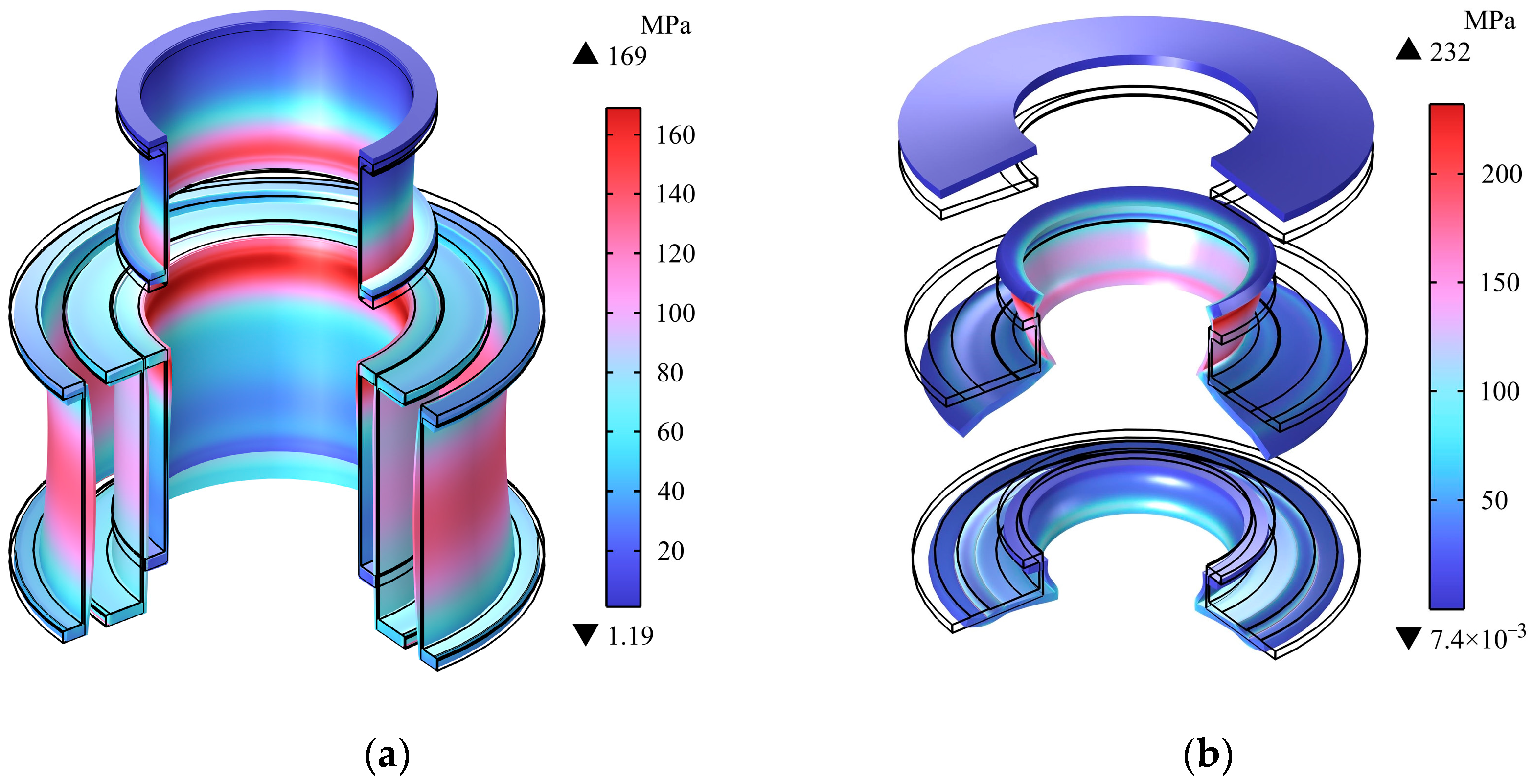
The calibration results for the equivalent stress of the mandrel and connecting block are illustrated in Figure 12. These figures reveal that the highest equivalent stress in the mandrel assembly part reaches 232 MPa. This value is lower than the permissible stress threshold of 316L stainless steel, which is 286 MPa at 4.2 K. The maximum stress predominantly occurs at the central region of the mandrel, specifically in the middle and upper parts of the connecting block.

Through calculation and simulation electromagnetic and stress analysis, the following conclusions are drawn: the magnet can be designed to operate stably in theory, and it is feasible to manufacture large-aperture high-field strong-gradient magnets with the structure described in this article.

5. Conclusions

This article presents the design of a gradient magnet with a maximum absolute gradient value of 400 T²/m. The room-temperature aperture of the gradient magnet is 200 mm, and it achieves a central magnetic field of 10.78 T. Employing a magnetic–force coupling method grounded in generalized stretching, the preload parameters of gradient coils are optimized through orthogonal parameter scanning. The study conducts a comprehensive analysis and calculation of the stress distribution in the magnet coils and mandrel. Key conclusions include the following: the electromagnetic design parameters of the magnet meet the design requirements; the stress–strain values of gradient magnet coils are within the permissible limits of their respective materials; the maximum equivalent stress in the mandrel assembly part is 232 MPa, which is below the permissible material stress of 286 MPa at 4.2 K. The peak stress is observed in the middle and upper part of the connecting block in the middle of the mandrel. From the results, there are two points to pay attention to in the design of large gradient magnets. Firstly, due to the influence of the electromagnetic distribution characteristics of gradient magnets, stress concentration may occur at the connection points of mechanical structures. If necessary, the structure can be strengthened. Secondly, in the design of gradient magnets, adding a pre tensioning layer can effectively reduce the electromagnetic stress in the system.

This article provides insights into magnet design optimization and stress–strain analysis methods in related fields. On a technical level, it can provide a reference for magnet design methods and stress calibration methods for researchers in the same field when designing similar high-gradient magnet structures. In terms of economic benefits, through finite element analysis, this design can save the costs in materials testing and stress testing or provide theoretical support. Meanwhile, the large-aperture high-field-strength gradient magnet designed in this study can generate considerable economic benefits in multiple fields such as life sciences, metal smelting, scientific research, semiconductors, and deep space exploration.