Abstract
Green roofs can be a valid solution for stormwater management in urban environments. The objective of this study was to develop a laboratory procedure for the hydraulic characterization of artificial substrates, used in the realization of green roofs, based on transient evaporation and steady-state unit hydraulic gradient (UHG) experiments. The retention, θ(h), and hydraulic conductivity, K(h), curves of two commercial substrates Terra Mediterranea® (TMT) and AgriTERRAM® (ATV) and a specifically developed substrate made by mixing peat, compost and sandy loam soil (MIX) were investigated. The unimodal van Genuchten–Mualem (VGM) hydraulic functions obtained by the direct evaporation method with different choices of the fitting parameters were compared with UHG measurements of K(h) conducted close to saturation. A numerical inversion of the transient evaporation experiments performed by Hydrus-1D software was also conducted, assuming that the hydraulic properties could be expressed either by unimodal or bimodal VGM models. The results indicated that an appropriate a priori choice of the residual water content parameter improved the estimation of the water retention curve. Moreover, the water retention data estimated from the direct evaporation method were not statistically different from those obtained with the inverse Hydrus-1D. The unsaturated hydraulic conductivity estimations obtained by the direct and inverse methods were highly correlated and the use of the bimodal VGM model improved the estimation of K(h) in the wet range. The numerical inversion of laboratory evaporation data with the hydraulic characteristics expressed by the bimodal VGM model proved to be a reliable and effective procedure for hydraulic characterization of artificial substrates, thus improving the reliability of simulated water fluxes in green roofs.
1. Introduction
Green roofs are low-impact development measures aimed at mitigating the effects of flooding in urban areas [1]. Green roofs are able to reduce and delay the peak rate into the sewage system through two mechanisms: (i) the retention of rainfall and (ii) the detention of runoff. The retention capacity is the volume of rainfall that is stored by the growing medium and lost via evapotranspiration. Detention refers to the temporal delay occurring between rainfall that is not retained and emerges as runoff [2]. Considering that roofs may represent a large portion of the total impervious surfaces in urban areas, green roofs are one of the key options for hydrologic restoration and stormwater management [3].
Conceptual models for green roof hydrologic functioning, e.g., [4], include lumped parameters that are case sensitive and need to be calibrated against experimental data, thus limiting their general applicability [5,6]. Physically based models such as Environmental Protection Agency (EPA)’s Storm Water Management Model (SWMM) [6,7], Soil Water Atmosphere and Plant (SWAP) model [8] and Hydrus model [9,10,11,12] in either one-dimensional [13,14], two-dimensional [15,16] and three-dimensional versions [5] were successfully applied to simulate the water balance and the hydrologic response of a vegetated roof. Knowledge of the hydraulic properties, i.e., the relationships between the soil water pressure head, h, the volumetric water content, θ, and the soil hydraulic conductivity, K, is necessary to apply simulation models based on the numerical solution of the Richards equation [8,14]. However, few studies have provided a comprehensive hydraulic characterization of green roof substrates. In most cases, the hydraulic properties of green roofs were highly simplified or limited to some specific soil characteristics (e.g., field capacity, wilting point, or particle size distribution) and generally focused only on the soil water retention curves. For example, in [13], only field capacity and wilting point were measured. These data, in conjunction with the bulk density and particle size distribution, were used to estimate the hydraulic properties of substrates using a pedotransfer function. Similarly, Refs. [8,17] assumed water retention parameters from the literature. Li and Babcock [15] acquired the shape parameters (α and n) of the van Genuchten model for water retention [18] from the hanging water column and saturated hydraulic conductivity from laboratory falling head experiments. A comprehensive estimation of both θ(h) and K(h) functions for a mineral green roof substrate was conducted by [5] and [14] who used a simplified version of the evaporation method with an extended measurement range [19,20]. However, they assumed the saturated soil hydraulic conductivity, Ks, as a fitting parameter and their estimations of soil hydraulic conductivity function basically relies on measurements conducted in the dry range between 10 and 30% of volumetric water content.
In the range of θ values near to soil saturation, an accurate determination of K(h) (or K(θ)) is critically important for highly permeable porous media, like green roof substrates, given they must ensure rapid drainage and avoid water ponding on the surface even during intense precipitation. However, the high non-linearity of hydraulic functions represents a major difficulty as a small change in θ may change K by several orders of magnitude.
A very effective and rapid transient laboratory method for simultaneous determination of both θ(h) and K(h) relationships for the same sample is the evaporation method, firstly proposed by Wind [21]. The water retention characteristic θ(h) is first estimated from the average water content and pressure head readings at several locations of the soil sample by an iterative procedure. Then, the unsaturated hydraulic conductivity function is determined from the pressure head profile and the changes in water content distribution. A simplified version of Wind’s method was proposed by [22] in which tensiometers are installed at only two depths within a short soil column. However, the linearizing assumptions of the simplified method with respect to time, space and the water content–pressure head relationship could result in marked deviations from the true hydraulic properties for the coarse-textured pore media that are commonly used for green roof design [23].
Apart from this, other limitations may affect the evaporation method. Water cavitation in the tensiometers, typically occurring around −70 to −90 kPa, limits the measurement range on the dry end [19,20]. On the wet end, the major limitations arise from the inability to obtain accurate estimates of the hydraulic conductivity because the hydraulic gradients are too small and subject to uncertainties in tensiometric readings [19,24]. However, many hydrologic and agronomic studies require soil hydraulic property measurements at both lower and higher tensions. Therefore, the integration of evaporation data with independent measurements conducted for both the wet and/or the dry ends seems a valuable solution to improve the soil hydraulic functions’ reliability. Water retention data at low pressure head values can be readily obtained by the pressure plate apparatus [25] whereas measurements of near-saturated hydraulic conductivity may be obtained from steady-state head-controlled infiltration experiments, like the unit hydraulic gradient (UHG) [26]. Although the combination of these two techniques is attractive, to our knowledge, measurements of near-saturated hydraulic conductivity on the same sample used for evaporation experiments were conducted only by [19,27]. Furthermore, provided that θ(h) and K(h) data collected from the evaporation method are generally fitted by closed-form empirical functions like the van Genuchten–Mualem (VGM) model [18], the consistency between modelled functions and additional steady-state measurements (pressure plate and UGH data) may be problematic and need to be specifically assessed. This is particularly true close to saturation where, due to the influence of the macropore domain, unimodal functions may be inappropriate to describe the hydraulic properties of green roof substrates [3,28,29,30].
Parameter optimization based on an inverse solution of the Richards equation has been largely used for soil hydraulic characterization (e.g., [31,32]). One of the advantages of the inverse method is the flexibility in modelling the hydraulic properties of the porous media. Though numerically more expensive, inverse modelling was considered preferable to simplified evaporation methods for coarse media with narrow pore-size distribution [33]. The optimization module of the Hydrus-1D model [9] was used to estimate the water retention curve and the hydraulic conductivity function of green roof substrates from simulated rainfall experiments [34,35,36,37] but the feasibility of estimating the parameters of the bimodal VGM [28] from an inverse approach was not explored.
The present study was performed with the main objective of developing a laboratory procedure for the hydraulic characterization of green roof artificial substrates based on evaporation and steady-state UHG experiments. The hydraulic properties of the substrates obtained with the direct Wind method were compared with those obtained by numerical inversion of the evaporation transient experiments performed by Hydrus-1D software. The agreement with independent near-saturated K measurements was assessed with the aim of establishing the reliability of unimodal and bimodal VGM models to describe the hydraulic properties of the considered artificial substrates. Specific aims were addressed, including the following: (i) evaluating the influence of fixing the parameters related to the dry portion of θ(h) and K(h) functions, namely the residual volumetric water content θr and the shape parameter λ, and (ii) establishing the best approach to obtain mean θ(h) and K(h) functions representative of several replicate samples.
2. Materials and Methods
2.1. Substrate Characteristics
Three green roof substrates were considered in this investigation, including two commercial substrates and a specifically developed growing substrate that showed good hydraulic characteristics for use in ornamental plant production [38]. The first commercial substrate is Terra Mediterranea® (TMT), manufactured by Harpo Verdepensile (Harpo spa, Trieste, Italy), consisting of a mixture of 80% mineral fraction (lapillus, pumice and zeolite) and 20% organic fraction (peat and compost). According to the technical specifications released by the manufacturer, the substrate dry bulk density, ρb, is 850–1000 kg m−3, the saturated hydraulic conductivity, Ks, is larger than 1200 mm h−1 and the field capacity (i.e., water content at 100 cm suction), θfc, is 0.30–0.45 m3m−3.The second commercial substrate is AgriTERRAM® TV (ATV) manufactured by Perlite Italiana srl (Corsico, Milan, Italy). The mineral fraction (75–80%) includes lapillus, pumice and expanded perlite and the organic fraction (20–25%) includes peat, bark, coconut fiber and organic conditioners. Technical specifications certify that ρb = 400 kg m−3, Ks > 780 mm h−1 and θfc > 0.50 m3m−3. The third growing substrate (MIX) was prepared by mixing on a volume basis 25% peat, 25% compost and 50% mineral soil. Commercial 100% sphagnum peat moss (Vigorplant, Fombio, Lodi, Italy) and 5-month-aged compost from orange juice processing wastes and garden cleaning [39] were used as organic fractions. The mineral fraction was obtained using 2 mm sieved sandy loam soil (Typic Rhodoxeralf, clay = 15.9%, silt = 27.2%, sand = 56.9%, USDA).
For each substrate, four replicated samples were prepared by compacting a given weight of material into plastic cylinders with a 9.3 cm inner diameter and 12 cm height. In order to avoid artefacts due to sample preparation, compaction was conducted in four successive steps by beating the substrates with five strokes from a height of 5 cm followed by five rotations with a pestle at each increment.
2.2. Evaporation and UHG Experiments
Given the evaporation method yields the drying branch of the unsaturated hydraulic functions (Figure 1a), the UHG experiment was performed prior to the evaporation experiment and following a descending sequence of applied pressure heads. A device similar to the one described by [26] was used (Figure 1b). Samples were saturated from the bottom on the porous plate of a glass funnel, with an air entry value of −40 cm, connected to an outflow tube that could be moved in height to establish a given h value at the bottom of the sample. A pressure head at the top of the sample was applied using a tension infiltrometer with an 8.5 cm diameter porous disk (Soil Measurement Systems, Tucson, AZ, USA). A thin layer of 2 mm sieved material was spread on the surface of TMT and ATV to ensure a good and stable hydraulic connection with the infiltrometer plate. The same h value was applied at both the upper and lower boundaries in order to establish and maintain a downward unit gradient flux. Under the assumption that the hydraulic gradient is a unit, the unsaturated hydraulic conductivity is equal to the measured downward steady-state flux. Steady-state conditions were considered to be achieved when the infiltration rate, at each imposed pressure head value, was constant with time. A sequence of pressure head values of −6, −12 and −18 cm was applied in succession.
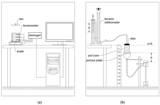
Figure 1.
Experimental setup for the Wind evaporation method (a) and apparatus for measuring unsaturated hydraulic conductivity with UHG method (b).
At the end of the UHG experiment, the sample bottom was sealed and three micro-tensiometers were horizontally inserted into holes drilled at 2, 6 and 10 cm heights in order to measure pressure head profiles during the evaporation experiment. The ceramic cups of 3 cm length and 0.6 cm outer diameter were connected to pressure transducers (SDEC, Reignac sur Indre, France). The soil core was then placed on a scale (maximum load 4000 g, resolution 0.1 g) and the evaporation process was allowed to start. Data from scales and tensiometers were automatically acquired and recorded by a CR1000 datalogger (Campbell Scientific, Shepshed, UK) at 1 min time intervals until the upper tensiometer stopped working properly. A blower was used to enhance the soil evaporation rate. For the entire duration of the evaporation experiments, the laboratory temperature was maintained at 22 ± 1 °C.
Depending on the characteristics of the tested substrates, the duration of evaporation experiments was from 72 to 170 hr for TMT, from 141 to 324 hr for ATV and from 222 to 489 h for MIX. The range of the explored pressure head values was rather limited, with the minimum measured h value equal to –282, –87 and –439 cm for TMT, ATV and MIX, respectively, but in line with the results obtained by [14] for TMT and [40] for coarse textured green roof substrates.
At the end of the experiment, the tensiometers were removed and the final water content of the substrate was determined by weighing the sample after oven drying at 105 °C. The average water contents of the soil sample at different times were backward calculated from recorded weights and final water content. For the calculation of hydraulic properties with the Wind iterative method [21], the soil core was divided into three compartments, centered on the tensiometer positions, with a constant thickness of 4 cm.
The volumetric water contents at a h value of −150 m, θ150, were determined by the pressure plate extractors on three replicated samples of 5-cm diameter by 1 cm height [25].
2.3. Determination of the Soil Hydraulic Functions
On the assumption that the soil column is homogeneous, determination of the water retention characteristic involved the following iterative procedure:
- An initial guess fitting of the van Genuchten [18] water retention curve was achieved from the mean values of the pressure head at the three depths, and the average sample water contents, , measured at the same time;
- Using the fitted water retention curve, water contents, θk,i, were estimated at depths and times at which the pressure heads were measured;
- The estimated average water contents were compared with the measured water storages of the soil sample obtained from weighting and the differences equally redistributed among the three compartments;
- From these θk,i vs. hk,i pairs, an updated water retention curve was obtained;
- Steps 3 and 4 were repeated until the maximum absolute change in water storage values between two successive iterations was < 0.0001 m3m−3.
In general, three iterations were sufficient to reach convergence.
Temporal changes in water content for each of the three compartments were used to compute hydraulic conductivity by means of a modified instantaneous profile method. During the time interval , the water flux, qk (L T−1) from the compartment k upward in the compartment k + 1 is approximated by:
in which Δz (L) is the compartment thickness (in this case Δz = 4 cm). The hydraulic conductivity, K (L T−1), was consequently computed according to the Darcy equation as follows:
where (∆h/∆z)k,k+1 is the average pressure head gradient between two consecutive compartments as measured from tensiometer readings at two consecutive times (ti and ti+1).
Corresponding h (or θ) values for the K(h) (or K(θ)) relationships were calculated from:
In view of the high uncertainty at low gradients due to the limited sensitivity of tensiometers, all K values obtained from hydraulic gradients lower than −0.2 m m−1 were excluded from the analysis.
2.4. Data Analysis
Coupled h vs. θ and K vs. h data obtained for each soil sample from the UHG and evaporation experiments were fitted by the unimodal van Genuchten–Mualem model [18] (VGM):
where Se is the effective water content, Ks (LT−1), is the saturated hydraulic conductivity, θr and θs (L3L−3) denote the residual and the saturated water contents, respectively, λ is a pore connectivity parameter, and α (L−1), n, and m (=1 − 1/n) are empirical parameters. Given that θr and λ influence the dry end of the soil hydraulic functions [41,42], it is likely that these parameters, when left unconstrained, could be poorly estimated. Therefore, it appeared worthwhile to evaluate if fixing θr and λ to an a priori fixed value could influence the quality of estimated θ(h) and K(h) functions.
In order to verify the role of fixing/estimating θr and λ parameters, the following preliminary analyses were conducted:
- 6.
- The retention data obtained by the evaporation method were fitted using Equation (5) considering α, n, and θs as fitting parameters, whereas θr was either fitted or fixed at θ150;
- 7.
- The hydraulic conductivity data obtained by the evaporation method were fitted using Equation (6) considering α, n, θs and θr values obtained from the previous step, Ks as a fitting parameter and λ either fitted or fixed at λ = 0.5.
The quality of fitting was evaluated for each substrate sample in terms of the Root Mean Square Error (RMSE) and Nash–Sutcliffe Efficiency (NSE) [43,44]. When the estimates obtained considering a different number of fitted parameters were compared, the Akaike’s information criterion (AIC) was also considered. The best fitting approach was selected as the one with the smallest value of AIC in order to penalize overfitting [5,45].
The possibility of estimating parameters of Equations (5) and (6) by the inverse method was also evaluated. To this aim, the sample weights and the pressure heads in the three compartments of the sample collected at 1 h intervals during the transient evaporation process were used as the input of the inverse method package of Hydrus-1D software [9]. Parameters α, n, and θs and Ks were estimated, while θr and λ were fixed at the optimal values obtained in the preceding step. Soil hydraulic properties obtained by the inverse method were compared with those obtained by the direct Wind method. Comparison was conducted either considering each replicated sample separately or the average θ(h) or K(h) curves obtained by the four replicates. Specifically, average θ(h) or K(h) curves were obtained by two approaches: (i) θ and K values were sampled at fixed h values (46 values for both θ and K) and averaged, the parameters of averaged θ(h) or K(h) curves were then obtained by fitting the VGM model; (ii) the VGM parameters of the four samples were averaged and a curve corresponding to the average parameters considered.
Finally, the mean K(h) relationships obtained from direct and inverse methods were compared with the mean near-saturated hydraulic conductivity values measured at −6, −12 and −18 cm by the UHG method. This last analysis aimed at evaluating the ability of the evaporation experiment when analyzed using the direct or inverse method to estimate accurate K values close to saturation. In order to increase the flexibility of θ(h) or K(h) function to fit the measured data, the bimodal van Genuchten–Mualem model was used as follows [28]:
where ω1 and ω2 are the weighting factors for the two flow regions (micro- and macropores), and αi, ni, mi (=1 − 1/ni), and λ are empirical parameters of the separate hydraulic functions (i = 1, 2).
3. Results
3.1. Estimation of Soil Hydraulic Functions by Direct Wind Method
The retention curves obtained for the different replicated samples of the three considered substrates are plotted in Figure 2. For both conditions (θr fitted or fixed at θ150), the estimated retention curves effectively reproduced the measured θ(h) values and the two curves mostly overlapped in the measurement range. The estimated values of the volumetric water content at saturation, θs, ranged from 0.46 to 0.48 cm3cm−3 and from 0.53 to 0.59 cm3cm−3 for the TMT and MIX substrates, respectively. For these substrates, the differences in θs estimated with the two procedures were the most equal to 0.01 cm3cm−3. It was concluded that a close estimation of θs can be obtained independently of the considered estimation strategy. The only exception was for two samples of the ATV substrate in which the difference between the two estimated θs values reached 0.09 cm3cm−3.
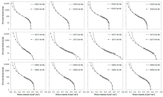
Figure 2.
Retention curves obtained for each sample of the three substrates (TMT, ATV and MIX) by assuming θr was fitted (θr = fit) or fixed at θ150 (θr = fix). The grey dots represent the measured values.
For all the considered experiments (n = 12), when θr was estimated (θr = fit), the iterative Wind procedure yielded θr = 0 as the best solution and, therefore, θr was fixed at zero. Compared to the θr = θ150 strategy, this resulted in a systematic underestimation of θ(h) in the dry range of the water retention curve. The goodness of fit for both strategies is indicated by the low RMSE values and the NSE value close to one. Specifically, the RMSE values ranged from a minimum of 0.002 to a maximum of 0.013 cm3cm−3, whereas the NSE index was always higher than 0.97.
For the TMT and ATV substrates, no clear preference for a specific estimation strategy could be claimed. For the MIX substrate, fixing the residual water content at the value measured for h = θ150 m generally yielded better estimates of the water retention curve (Table 1). From these findings, it can be deduced that the estimation of the retention curve carried out with the direct Wind method is more accurate if an appropriate choice of the θr parameter is made.

Table 1.
Parameters of the retention curves obtained by the direct Wind method by assuming θr was fitted or fixed at θ150.
The measured values of unsaturated soil hydraulics showed a large dispersion at higher pressure heads (h > −30 cm) particularly for the two commercial substrates (TMT and ATV) (Figure 3). The uncertainty in K(h) measurements close to saturation is a known drawback of the evaporation method due to the influence of measurement errors when the hydraulic gradients are low. In the case of the commercial substrate, the measurement error influence is probably emphasized by the coarser nature of the material that makes the hydraulic contact with the ceramic cup of the tensiometers more problematic.
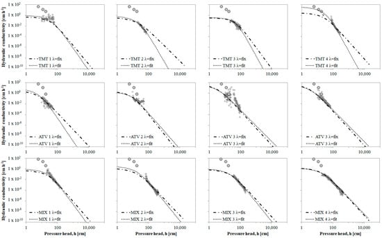
Figure 3.
Hydraulic conductivity curves obtained for each sample of the three substrates by considering λ fitted (λ = fit) or fixed at 0.5 (λ = fix). The grey crosses and dots represent the values measured by direct Wind and UGH methods, respectively.
For both the considered conditions (λ fitted or fixed at 0.5), the estimated hydraulic conductivity curves overlapped the experimental K(h) values in the measured range of pressure heads (Figure 3). The two estimated K(h) relationships diverged for drier conditions (i.e., low h values). In this range, fitting of the λ parameter generally resulted in an underestimation of the unsaturated hydraulic conductivity function. This was the case for TMT, for which λ ranged from 1.51 to 6.57, sample 1 of ATV (λ = 3.0) and samples 1, 2 and 3 of MIX (λ = 1.32–1.77). Conversely, overestimated K(h) functions in the dry range corresponded to fitted values of λ lower than 0.5 (samples 2, 3 and 4 of ATV and sample 4 of MIX). Due to the direct correlation existing between Ks and λ [32,46], higher estimated saturated hydraulic conductivity values corresponded to higher λ values (Table 2). Fitting a λ parameter greater than 0.5 resulted in an overestimation of Ks by a mean factor of 3.1. When fitted λ was lower than 0.5, Ks was underestimated by a mean factor of 0.87. Therefore, overestimation of Ks when λ was left unconstrained was a more frequent and relevant outcome than the opposite one (underestimation of Ks). It is worth noting that even an overestimation of Ks up to a factor of 2 was not able to fit the near saturated hydraulic conductivity values estimated from UHG experiments (Figure 3). The only exception was for sample 4 of TMT, for which Ks estimated with unconstrained λ was a factor of 12.4 larger than the one estimated with λ = 0.5.
Table 2.
Parameters of hydraulic conductivity curves obtained with the Wind iterative approach by assuming λ fitted or fixed at 0.5.
The RMSE and NSE values indicated a very good estimation performance for the MIX substrate and a relatively good performance for the other two substrates (Table 2). Only sample 1 of TMT showed negative values of NSE and high values of RMSE. In terms of RMSE and NSE, the two considered estimation strategies (λ fitted or fixed at 0.5) were practically equivalent. For 10 out of 12 samples, the AIC values for fitted λ were lower than those for fixed λ. The two exceptions were sample 1 of TMT and sample 3 of ATV that showed poor RMSE and NSE values. Therefore, the strategy involving fitting of the λ parameter was considered preferable to that assuming a constrained λ value equal to 0.5.
3.2. Estimation of Soil Hydraulic Functions by Inverse Method
The retention and hydraulic conductivity curve parameters of three substrates estimated by the inverse method applied to the evaporation experiments are shown in Table 3. According to the results of the previous section, the θr parameter was set at θ150 and the λ parameter was estimated. Comparison between the mean soil hydraulic parameters obtained by the direct and inverse methods is reported in Table 4.
Table 3.
Parameters of retention and hydraulic conductivity curves obtained by applying the inverse method approach.
Table 4.
Soil hydraulic parameters obtained by the direct Wind method and the inverse Hydrus-1D method by considering two averaging approaches.
The parameters of the water retention curves (i.e., α, n, and θs) obtained as the mean of the parameters of Equation (5) fitted to the individual samples were practically identical to those obtained by fitting Equation (5) to the mean water retention data. Minor differences in the two averaging approaches were found for hydraulic conductivity function parameters (Ks and λ). However, the differences in estimated Ks were reported within a factor of 0.96–1.04 that is negligible in practice. It was concluded that the two averaging approaches yielded coincident estimations of the substrate hydraulic properties as far as the unimodal VGM model is considered.
The retention curves and hydraulic conductivity functions obtained for the single samples of the three substrates with the direct and inverse method are compared in Figure 4. The plots confirm the good agreement of water retention curve estimates obtained by the direct and inverse methods with coefficients of determination, R2, that ranged between 0.9768 and 1.00 (Table 5). On average, the best agreement between the water retention curve estimated by the two methods (i.e., direct and inverse) was observed for the MIX substrate (mean R2 = 0.9997) and the worst for the TMT substrate (mean R2 = 0.9973). The correlation for the hydraulic conductivity function was generally lower than the water retention curve, confirming that the two methods could yield different results for K(h) (Table 5). The largest discrepancies were observed for substrate TMT with a mean R2 of 0.9741. The remaining substrates were characterized by similar mean R2 values (R2 = 0.9915 for ATV and R2 = 0.9916 for MIX). It is worth noting, however, that the worse correspondence observed for the TMT substrate is mostly determined by a single sample (sample TMT 1) that resulted in a very different estimation of λ parameters with the two approaches.
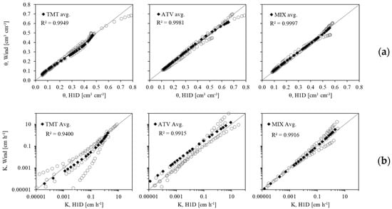
Figure 4.
Comparison between (a) volumetric water content θ and (b) hydraulic conductivity K values estimated for a given h value by the direct Wind and inverse Hydrus-1D methods. Symbols in grey represent the individual samples, while symbols in black represent the average values.
Table 5.
Correlation parameters for the water retention and hydraulic conductivity curves obtained from direct Wind and inverse Hydrus-1D methods.
The results demonstrated how the two methods of analysis of the evaporation tests yielded similar results both in terms of the estimated water retention curve and unsaturated hydraulic conductivity functions. However, even with the inverse method, the marked tendency to underestimate the near saturated hydraulic conductivity measured with the UHG method was confirmed.
The bimodal VGM model was used in order to improve the predictive ability of the inverse Hydrus-1D method at high-pressure head values (Table 6). Due to the increased flexibility of the bimodal hydraulic functions, higher values of Ks were obtained that better approached the independently measured values. At the same time, larger λ values were estimated (Table 6). For the TMT substrate, Ks values estimated by the inverse method and the bimodal VGM model ranged from 54.1 to 473.4 cm h−1 with an average value of 182.4 cm h−1. For the ATV substrate, estimated Ks values ranged from 75.3 to 315.7 cm h−1 with an average value of 235.4 cm h−1. Finally, for the MIX substrate, the estimated Ks values were between 135.8 and 315.6 cm h−1 with an average value of 179.2 cm h−1.
Table 6.
Parameters of the van Genuchten bimodal water retention (Equation (7)) and hydraulic conductivity (Equation (8)) functions obtained by the inverse method.
The mean hydraulic conductivity curves obtained by the inverse method considering unimodal and bimodal unsaturated hydraulic conductivity functions are plotted in Figure 5. Compared to the unimodal model, the bimodal model was more effective in fitting the experimental data points obtained with the UHG method at a pressure head close to zero.
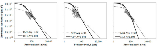
Figure 5.
Hydraulic conductivity curves obtained by the inverse method considering unimodal (Equations (5) and (6), dot line) and bimodal (Equations (7) and (8), continuous line) VGM models. Lines represent the average of four replicated samples. Grey crosses and dots represent the measured K(h) values of individual samples measured by direct Wind and UGH methods, respectively.
4. Discussion
The direct Wind [21] evaporation method with a pressure head measured at three heights allowed an accurate description of the unimodal water retention curve of the three considered substrates, provided the θr parameter is fixed at the water content value measured at h = −150 m. Despite showing a relative larger dispersion at high h values, the measured unsaturated hydraulic conductivity data were adequately fitted by the unimodal VGM model when the λ parameter was left unconstrained. The direct Wind and the inverse Hydrus-1D methods yielded estimations of the water retention data that were practically coincident and highly correlated (R2 > 0.97) estimations of K(h). The experimental setup consisting of three tensiometers at 4 cm intervals seemed adequate to estimate the hydraulic properties of coarse green roof substrates that may be problematic with the simplified evaporation method, making use of only two tensiometers [23,33]. A very good estimation performance for the MIX substrate and a relatively good performance for the coarser TMT and ATV substrates was obtained, thus confirming that this sample schematization improved identification of the non-linearity of h(t) profiles in the initial stage of the transient process and reduced errors caused by linearization and quasi steady-state assumptions [24]. However, for pressure heads higher than −30 cm, direct measurement of K(h) was inaccessible due to the estimates of the hydraulic gradient that become too small. This is a well-known limitation of the evaporation method that can be overcome by conducting UHG and evaporation experiments in succession on the same sample [20,27]. However, our results showed that this strategy was not enough in the case of green roof substrates that present a heterogeneous composition with a double order of pores of different sizes, i.e., micropores and macropores [30]. Indeed, the independently measured hydraulic conductivity values close to saturation were always underestimated.
When the inverse method with the hydraulic properties expressed by the bimodal VGM model was used, a close description of the K(h) function in the range from saturation to the lower limit of the evaporation method was obtained. The effective benefit of using the bimodal VGM model was sometimes questioned. Peng et al. [3] and Liu and Fassman-Beck [29] showed that the bimodal VGM model improved the description of substrates’ water retention but the hydraulic conductivity was effectively improved only when a three-modal function was considered. Turco et al. [30] showed that although the substrate could have a bimodal behavior, the differences between uni- and bimodal soil hydraulic characteristics had minimal effects on the hydrological functioning of a green roof, given the error in simulated runoff volume is less than 1%. They concluded that the unimodal model must be preferred instead of the bimodal due to the lower number of estimated parameters.
5. Conclusions
The knowledge of the substrate hydraulic properties, i.e., the relationships between the water pressure head, h, the volumetric water content, θ, and the hydraulic conductivity, K, of the porous medium, is crucial for the simulation of water fluxes in green roofs by mechanistic models. The evaporation method could be a very effective and rapid transient laboratory method for simultaneous determination of θ(h) and K(h) relationships. In this study, we applied the Wind evaporation method supplemented by steady-state independent measurements of K(h) conducted close to saturation to estimate the hydraulic properties of artificial substrates designed for green roof preparation. The results confirmed that the evaporation method, either direct or inverse, is inadequate to estimate the near saturated hydraulic conductivity of heterogeneous pore media like the substrates under study. A much better description of the K(h) function could be obtained only when the inverse method with the bimodal VGM model was used. Therefore, this approach could be recommended as an effective strategy for green roof substrate characterization.
However, further investigation is necessary to assess the effectiveness of the bimodal models in improving the simulation of the hydraulic processes that occur in extensive green roofs subjected to natural rainfall and evapotranspiration.
Author Contributions
Conceptualization, M.I.; methodology, D.A., V.A. and C.B.; formal analysis, D.A. and V.A.; investigation, D.A., V.A. and C.B.; data curation, D.A. and M.I.; writing—original draft preparation, D.A. and M.I.; writing—review and editing, D.A., V.A., C.B. and M.I. All authors have read and agreed to the published version of the manuscript.
Funding
This research was funded by the European Union—FESR or FSE, PON Research and Innovation 2014–2020—DM 1062/2021 and PRIN 2022 PNRR “NBS4STORWATER”, Next Generation EU, M4C2, CUP B53D23023760001.
Institutional Review Board Statement
Not applicable.
Informed Consent Statement
Not applicable.
Data Availability Statement
The raw data supporting the conclusions of this article will be made available by the authors on request.
Conflicts of Interest
The authors declare no conflicts of interest.
References
- Czemiel Berndtsson, J. Green Roof Performance towards Management of Runoff Water Quantity and Quality: A Review. Ecol. Eng. 2010, 36, 351–360. [Google Scholar] [CrossRef]
- Stovin, V.; Poë, S.; De-Ville, S.; Berretta, C. The Influence of Substrate and Vegetation Configuration on Green Roof Hydrological Performance. Ecol. Eng. 2015, 85, 159–172. [Google Scholar] [CrossRef]
- Peng, Z.; Smith, C.; Stovin, V. The Importance of Unsaturated Hydraulic Conductivity Measurements for Green Roof Detention Modelling. J. Hydrol. 2020, 590, 125273. [Google Scholar] [CrossRef]
- Kasmin, H.; Stovin, V.R.; Hathway, E.A. Towards a Generic Rainfall-Runoff Model for Green Roofs. Water Sci. Technol. 2010, 62, 898–905. [Google Scholar] [CrossRef] [PubMed]
- Brunetti, G.; Šimůnek, J.; Piro, P. A Comprehensive Analysis of the Variably Saturated Hydraulic Behavior of a Green Roof in a Mediterranean Climate. Vadose Zone J. 2016, 15, vzj2016-04. [Google Scholar] [CrossRef]
- Peng, Z.; Garner, B.; Stovin, V. Two Green Roof Detention Models Applied in Two Green Roof Systems. J. Hydrol. Eng. 2022, 27, 04021049. [Google Scholar] [CrossRef]
- Krebs, G.; Kuoppamäki, K.; Kokkonen, T.; Koivusalo, H. Simulation of Green Roof Test Bed Runoff. Hydrol. Process 2016, 30, 250–262. [Google Scholar] [CrossRef]
- Metselaar, K. Water Retention and Evapotranspiration of Green Roofs and Possible Natural Vegetation Types. Resour. Conserv. Recycl. 2012, 64, 49–55. [Google Scholar] [CrossRef]
- Simunek, J.; Sejna, M.; Saito, H.; Sakai, M.; van Genuchten, M.T. The HYDRUS-1D Software Package for Simulating the One-Dimensional Movement of Water, Heat, and Multiple Solutes in Variably-Saturated Media; Version 4.08. HYDRUS Softw. Ser. 3; University of California-Riverside Research Reports: Riverside, CA, USA, 2009. [Google Scholar]
- Simunek, J.; Van Genuchten, M.T.; Sejna, M. The HYDRUS Software Package for Simulating the Two- and Three-Dimensions Movement of Water, Heat, and Multiple Solutes in Variably-Saturated Media. Tech. Man. 2011, 1, 241. [Google Scholar]
- Ghazouani, H.; M’Hamdi, B.D.; Autovino, D.; Bel Haj, A.M.; Rallo, G.; Provenzano, G.; Boujelben, A. Optimizing Subsurface Dripline Installation Depth with Hydrus 2D/3D to Improve Irrigation Water Use Efficiency in the Central Tunisia. Int. J. Metrol. Qual. Eng. 2015, 6, 402. [Google Scholar] [CrossRef]
- Basile, A.; Albrizio, R.; Autovino, D.; Bonfante, A.; De Mascellis, R.; Terribile, F.; Giorio, P. A Modelling Approach to Discriminate Contributions of Soil Hydrological Properties and Slope Gradient to Water Stress in Mediterranean Vineyards. Agric. Water Manag. 2020, 241, 106338. [Google Scholar] [CrossRef]
- Hilten, R.N.; Lawrence, T.M.; Tollner, E.W. Modeling Stormwater Runoff from Green Roofs with HYDRUS-1D. J. Hydrol. 2008, 358, 288–293. [Google Scholar] [CrossRef]
- Palermo, S.A.; Turco, M.; Principato, F.; Piro, P. Hydrological Effectiveness of an Extensive Green Roof in Mediterranean Climate. Water 2019, 11, 1378. [Google Scholar] [CrossRef]
- Li, Y.; Babcock, R.W. Modeling Hydrologic Performance of a Green Roof System with HYDRUS-2D. J. Environ. Eng. 2015, 141, 04015036. [Google Scholar] [CrossRef]
- Brunetti, G.; Šimůnek, J.; Turco, M.; Piro, P. On the Use of Surrogate-Based Modeling for the Numerical Analysis of Low Impact Development Techniques. J. Hydrol. 2017, 548, 263–277. [Google Scholar] [CrossRef]
- Palla, A.; Gnecco, I.; Lanza, L.G. Unsaturated 2D Modelling of Subsurface Water Flow in the Coarse-Grained Porous Matrix of a Green Roof. J. Hydrol. 2009, 379, 193–204. [Google Scholar] [CrossRef]
- van Genuchten, M.T. A Closed-Form Equation for Predicting the Hydraulic Conductivity of Unsaturated Soils. Soil Sci. Soc. Am. J. 1980, 44, 892–898. [Google Scholar] [CrossRef]
- Schindler, U.; Durner, W.; von Unold, G.; Müller, L. Evaporation Method for Measuring Unsaturated Hydraulic Properties of Soils: Extending the Measurement Range. Soil Sci. Soc. Am. J. 2010, 74, 1071–1083. [Google Scholar] [CrossRef]
- Schindler, U.; Durner, W.; von Unold, G.; Mueller, L.; Wieland, R. The Evaporation Method: Extending the Measurement Range of Soil Hydraulic Properties Using the Air-Entry Pressure of the Ceramic Cup. J. Plant Nutr. Soil Sci. 2010, 173, 563–572. [Google Scholar] [CrossRef]
- Wind, G.P. Capillary Conductivity Data Estimated by a Simple Method. In Water in the Unsaturated Zone, Proceedings of Wageningen Symposium; Institute for Land and Water Management Research: Wageningen, The Netherlands, 1969; Volume 1, p. 1. [Google Scholar]
- Schindler, U. Ein Schnellverfahren Zur Messung Der Wasserleitfähigkeit Im Teilgesättigten Boden an Stechzylinderproben. Arch. Acker Pflanzenbau Bodenkd. 1980, 24, 1–7. [Google Scholar]
- Peters, A.; Iden, S.C.; Durner, W. Revisiting the Simplified Evaporation Method: Identification of Hydraulic Functions Considering Vapor, Film and Corner Flow. J. Hydrol. 2015, 527, 531–542. [Google Scholar] [CrossRef]
- Peters, A.; Durner, W. Simplified Evaporation Method for Determining Soil Hydraulic Properties. J. Hydrol. 2008, 356, 147–162. [Google Scholar] [CrossRef]
- Dane, J.H.; Hopmans, J.W. Pressure Plate Extractor. In Methods of Soil Analysis, Part 4, Physical Methods; Dane, J.H., Topp, G.C., Eds.; Soil Science Society of America, Inc.: Madison, WI, USA, 2002; pp. 680–683. [Google Scholar]
- Bagarello, V.; Castellini, M.; Iovino, M. Comparison of Unconfined and Confined Unsaturated Hydraulic Conductivity. Geoderma 2007, 137, 394–400. [Google Scholar] [CrossRef]
- Sarkar, S.; Germer, K.; Maity, R.; Durner, W. Measuring Near-Saturated Hydraulic Conductivity of Soils by Quasi Unit-Gradient Percolation—2. Application of the Methodology. J. Plant Nutr. Soil Sci. 2019, 182, 535–540. [Google Scholar] [CrossRef]
- Durner, W. Hydraulic Conductivity Estimation for Soils with Heterogeneous Pore Structure. Water Resour. Res. 1994, 30, 211–223. [Google Scholar] [CrossRef]
- Liu, R.; Fassman-Beck, E. Pore Structure and Unsaturated Hydraulic Conductivity of Engineered Media for Living Roofs and Bioretention Based on Water Retention Data. J. Hydrol. Eng. 2018, 23, 04017065. [Google Scholar] [CrossRef]
- Turco, M.; Palermo, S.A.; Polizzi, A.; Presta, L.; Pirouz, B.; Piro, P. The Assessment of the Effectiveness of the Unimodal and Bimodal Models to Evaluate the Water Flow through Nature-Based Solutions Substrates. Water Sci. Technol. 2023, 88, 932–946. [Google Scholar] [CrossRef] [PubMed]
- Šimůnek, J.; van Genuchten, M.T.; Wendroth, O. Parameter Estimation Analysis of the Evaporation Method for Determining Soil Hydraulic Properties. Soil Sci. Soc. Am. J. 1998, 62, 894–905. [Google Scholar] [CrossRef]
- Crescimanno, G.; Iovino, M. Parameter Estimation by Inverse Method Based on One-Step and Multi-Step Outflow Experiments. Geoderma 1995, 68, 257–277. [Google Scholar] [CrossRef]
- Iden, S.C.; Blöcher, J.R.; Diamantopoulos, E.; Peters, A.; Durner, W. Numerical Test of the Laboratory Evaporation Method Using Coupled Water, Vapor and Heat Flow Modelling. J. Hydrol. 2019, 570, 574–583. [Google Scholar] [CrossRef]
- Huang, S.; Garg, A.; Mei, G.; Huang, D.; Chandra, R.B.; Sadasiv, S.G. Experimental Study on the Hydrological Performance of Green Roofs in the Application of Novel Biochar. Hydrol. Process 2020, 34, 4512–4525. [Google Scholar] [CrossRef]
- Wang, J.; Garg, A.; Liu, N.; Chen, D.; Mei, G. Experimental and Numerical Investigation on Hydrological Characteristics of Extensive Green Roofs under the Influence of Rainstorms. Environ. Sci. Pollut. Res. 2022, 29, 53121–53136. [Google Scholar] [CrossRef]
- Bouzouidja, R.; Séré, G.; Claverie, R.; Ouvrard, S.; Nuttens, L.; Lacroix, D. Green Roof Aging: Quantifying the Impact of Substrate Evolution on Hydraulic Performances at the Lab-Scale. J. Hydrol. 2018, 564, 416–423. [Google Scholar] [CrossRef]
- Gan, L.; Garg, A.; Wang, H.; Mei, G.; Liu, J. Influence of Biochar Amendment on Stormwater Management in Green Roofs: Experiment with Numerical Investigation. Acta Geophys. 2021, 69, 2417–2426. [Google Scholar] [CrossRef]
- Gugliuzza, G.; Verduci, A.; Iovino, M. Water Retention Characteristics of Substrates Containing Biochar and Compost as Peat and Perlite Replacements for Ornamental Plant Production. Acta Hortic. 2021, 1305, 507–512. [Google Scholar] [CrossRef]
- Bondì, C.; Castellini, M.; Iovino, M. Compost Amendment Impact on Soil Physical Quality Estimated from Hysteretic Water Retention Curve. Water 2022, 14, 1002. [Google Scholar] [CrossRef]
- Sandoval, V.; Bonilla, C.A.; Gironás, J.; Vera, S.; Victorero, F.; Bustamante, W.; Rojas, V.; Leiva, E.; Pastén, P.; Suárez, F. Porous Media Characterization to Simulate Water and Heat Transport through Green Roof Substrates. Vadose Zone J. 2017, 16, 1–14. [Google Scholar] [CrossRef]
- Nimmo, J.R. Comment on the Treatment of Residual Water Content in “A Consistent Set of Parametric Models for the Two-phase Flow of Immiscible Fluids in the Subsurface” by L. Luckner et Al. Water Resour. Res. 1991, 27, 661–662. [Google Scholar] [CrossRef]
- Shinomiya, Y.; Takahashi, K.; Kobiyama, M.; Kubota, J. Evaluation of the Tortuosity Parameter for Forest Soils to Predict Unsaturated Hydraulic Conductivity. J. For. Res. 2001, 6, 221–225. [Google Scholar] [CrossRef]
- Moriasi, D.N.; Arnold, J.G.; Van Liew, M.W.; Bingner, R.L.; Harmel, R.D.; Veith, T.L. Model Evaluation Guidelines for Systematic Quantification of Accuracy in Watershed Simulations. Trans. ASABE 2007, 50, 885–900. [Google Scholar] [CrossRef]
- Duc, L.; Sawada, Y. A Signal-Processing-Based Interpretation of the Nash-Sutcliffe Efficiency. Hydrol. Earth Syst. Sci. 2023, 27, 1827–1839. [Google Scholar] [CrossRef]
- Jarvis, N.; Koestel, J.; Messing, I.; Moeys, J.; Lindahl, A. Influence of Soil, Land Use and Climatic Factors on the Hydraulic Conductivity of Soil. Hydrol. Earth Syst. Sci. 2013, 17, 5185–5195. [Google Scholar] [CrossRef]
- Weynants, M.; Vereecken, H.; Javaux, M. Revisiting Vereecken Pedotransfer Functions: Introducing a Closed-Form Hydraulic Model. Vadose Zone J. 2009, 8, 86–95. [Google Scholar] [CrossRef]
Disclaimer/Publisher’s Note: The statements, opinions and data contained in all publications are solely those of the individual author(s) and contributor(s) and not of MDPI and/or the editor(s). MDPI and/or the editor(s) disclaim responsibility for any injury to people or property resulting from any ideas, methods, instructions or products referred to in the content. |
© 2024 by the authors. Licensee MDPI, Basel, Switzerland. This article is an open access article distributed under the terms and conditions of the Creative Commons Attribution (CC BY) license (https://creativecommons.org/licenses/by/4.0/).