Towards Real-Time Machine Learning-Based Signal/Background Selection in the CMS Detector Using Quantized Neural Networks and Input Data Reduction

Abstract

The Large Hadron Collider (LHC) is being prepared for an extensive upgrade to boost its particle discovery potential. The new phase, High Luminosity LHC, will operate at a factor-of-five-increased luminosity (the number proportional to the rate of collisions). Consequently, such an increase in luminosity will result in enormous quantities of generated data that cannot be transmitted or stored with the currently available resources and time. However, the vast majority of the generated data consist of uninteresting data or pile-up data containing few interesting events or electromagnetic showers. High-Luminosity LHC detectors, including the Compact Muon Solenoid (CMS), will thus have to rely on innovative approaches like the proposed one to select interesting collision data. In charge of data reduction/selection at the early stages of data streaming is a level 1 trigger (L1T), a real-time event selection system. The final step of the L1T is a global trigger, which uses sub-system algorithms to make a final decision about signal acceptance/rejection within a decision time of around 12 microseconds. For one of these sub-system L1T algorithms, we propose using quantized neural network models deployed in targeted L1T devices, namely, field-programmable gate arrays (FPGA), as a classifier between electromagnetic and pile-up/quantum chromodynamics showers. The developed quantized neural network operates in an end-to-end manner using raw detector data to speed up the classification process. The proposed data reduction methods further decrease model size while retaining accuracy. The proposed approach was tested with simulated data (since the detector is still in the production stage) and took less than 1 microsecond, achieving real-time signal–background classification with a classification accuracy of $97.37$% for 2-bit-only quantization and $97.44$% for quantization augmented with the data reduction approach (compared to $98.61$% for the full-precision, standard network).

1. Introduction

Exploration of the essential nature of space and discoveries of exotic particles would not be possible without particle accelerators, which are primary tools in high-energy physics (HEP). The world’s largest particle accelerator, the Large Hadron Collider (LHC) [1], is built to understand the fundamental laws of nature and test different predictions of elementary particle physics. In 2012, the LHC experiments A Toroidal LHC Apparatus and Compact Muon Solenoid (CMS) [2] confirmed the existence of the Higgs boson through the discovery of the predicted fundamental particle. The current phase aims to fully characterize the Higgs boson properties and search for phenomena beyond the standard model.

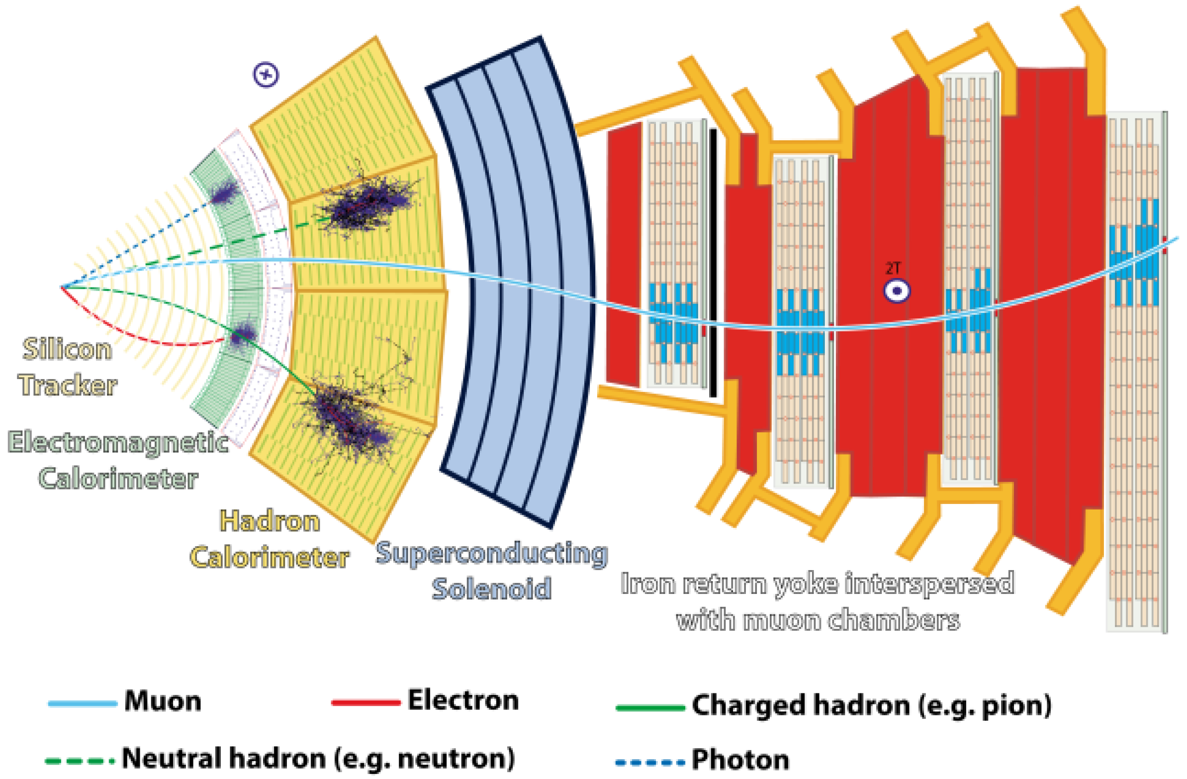
In the LHC ring, high-energy proton collisions occur every 25 ns. To analyze the results of the collisions, four detectors surround collision points and record the obtained data. One of four LHC detectors is CMS, a cylindrically shaped general-purpose detector with several concentric layers of components (Figure 1). When interesting particles are produced as a result of the collision, they immediately decay into lighter, stable particles. As shown in Figure 1, decay products pass through detector layers and interact with them, allowing their direction and momentum to be measured. Among the detectable decay products, there are electrically charged leptons (electrons and muons) and particle jets (collimated streams of particles originating from quarks and gluons) [3].

The CMS is undergoing a major upgrade for the High-Luminosity (HL)-LHC era, and one of the most important enhancements is the design of the high-granularity calorimeter (HGCAL) [5], a radiation-hard replacement of endcaps. It is a sampling calorimeter characterized by very-high granularity using 6 million silicon and 400 thousand scintillator channels. Silicon cells are fine-segmented, radiation tolerant, and fast enough to mitigate PU. Hence, they will be used as active elements in high-radiation areas, and, to reduce cost, scintillators will be used as active elements in lower-radiation areas (Figure 2). The HGCAL consists of an electromagnetic part (CE-E) containing 14 layers of hexagonal silicon sensors, which alternate with absorber layers made of lead, copper–tungsten, and copper. The hadronic part (CE-H) consists of another 8 silicon layers and 14 mixed layers with silicon and scintillator. 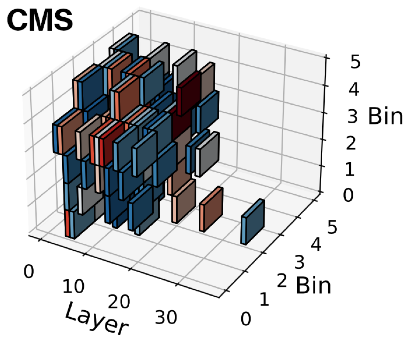At the moment when the experiment presented herein was initiated, there were a total of 50 layers set to be used in HGCAL [6], as was planned to be used in the experiment. In the recent design revision, the number of layers was reduced to 47 [7] but could also be changed up until actual production.

This paper concentrates on the electromagnetic calorimeter sub-detector part, where particles such as electrons and photons are detected. Combining the data coming from different sub-detectors, the ultimate goal was to obtain a complete picture of the collision event and enable the application of a wide range of physical analyses. However, due to the high rate of collisions (40 MHz), the detector produces tens of terabytes of data per second, exceeding the available processing and storage resources. Thus, the crucial part of the CMS dataflow consists of the event data selection algorithms in the early dataflow stage. Such algorithms should decide which data are potentially interesting, enabling transmission of only those data for more detailed analysis (and irretrievably rejecting the rest) while adhering to strict resource constraints (in terms of power, time, storage, and bandwidth). This process is overseen by an event-processing system called level 1 trigger (L1T), which runs in real-time and requires a fast decision on the input data stream. The decision will be even more demanding in the HL-LHC phase because of the increased luminosity, the unprecedented radiation dose, and the vast majority of uninteresting additional proton–proton interactions referred to as pile-up (PU). Thus, the purpose of this paper is not a physical analysis but the introduction of input data reduction algorithms, as well as the implementation of a real-time model for signal versus background classification.

An expected increase in the data rate for the HL-LHC requires advanced approaches that would enable efficient real-time analysis methods for the HGCAL L1 trigger. Artificial intelligence, especially machine learning (ML), has become a standard tool in analyzing big data and is gradually becoming a common tool in HEP. The development of sophisticated ML algorithms, specifically convolutional neural networks (CNN), has been shown as a powerful tool in image recognition, solving many computer vision problems. Until recently, the main drawback of real-time implementation was the fact that running capable ML methods requires time and powerful hardware. Advanced approaches have enabled the integration of ML methods in real-time processing tasks [8,9,10].

Figure 2. The HGCAL endcap mechanical construction (left) and a single electromagnetic and hadronic calorimeter layer (right), adjusted from [5,11].

Figure 2. The HGCAL endcap mechanical construction (left) and a single electromagnetic and hadronic calorimeter layer (right), adjusted from [5,11].

However, in restricted conditions under which the collection and primary selection of data take place inside the LHC detectors, the standard hardware and operating systems used for typical ML applications are not possible to use. Because of radiation exposure, restricted budget, the possibility of material damage, and the enormous data rate, a choice has been made on field-programmable gate arrays (FPGAs) to be used as a platform for L1 trigger algorithms. Compared to central processing units or graphic processing units, they are very efficient because of very high throughput, low latency, and low power budget. Recently, scientists have begun to explore using ML techniques, specifically neural networks (NN), on FPGAs to improve real-time event processing. This paper deals with the same topic and presents a case study for real-time signal/background classification of the HGCAL data using quantized neural networks deployed on FPGAs. The reason behind network quantization is an effort to reduce the network requirements since limited resources are available on the target FPGA, shared between multiple algorithms. Moreover, input data reduction is applied using selection and quantization procedures to additionally decrease the model size and reduce latency and memory requirements.

This paper is organized as follows. Section 2 describes the application of NN in HEP, particularly for triggering purposes in particle detectors. Section 3 presents the methodology of the conducted study: the process of generating the image data set is described, together with details of NN model optimization. The section ends with the introduction to the hls4ml tool. Section 4 illustrates the performance of the described models via several data refinement approaches and comparisons with baseline particle classification methods. The results of the implementation of selected models in FPGA using hls4ml are discussed at the end of the section. Section 5 concludes the paper, followed by the references used. Readers should also note that, before the References, a brief Glossary of physics-related terms used throughout this manuscript is included. Understanding these terms is not critical to solving the engineering challenges that the manuscript addresses, but it should aid the interested reader with the manuscript’s readability.

2. Previous Work

This section is divided into four main parts, reflecting the different (but interconnected) topics under consideration. The first part is dedicated to exploring the different applications of NNs in HEP, encompassing particle identification, tracking, and event classification, among others. The second part provides an extensive overview of the historical usage of low-level data for NN implementation in HEP. This section also highlights the connection between detector data and image pixels and gives examples of its usage. The third part, “Neural Networks for Triggering”, offers a history of NN usage in HEP for both levels of the trigger system. The fourth and final part, “Neural Network Quantization”, comprehensively addresses NN quantization, detailing the available approaches.

When reviewing similar work, the reader should keep in mind that the NN models presented in the review use entirely different datasets and types of features to make predictions for their respective applications (some of which are similar to ours). As a result, directly comparing the accuracy or efficiency of one ML model to another (either ours or models from other studies) is not a straightforward process. Each model is optimized to be used for a specific set of features; therefore, the comparison of their performance must also be based on the same criteria. Failure to do so could result in misleading conclusions that do not accurately reflect the true capabilities of the models.

2.1. Applications of Neural Networks in HEP

Because of their efficiency in processing large amounts of data, ML techniques have been used frequently in HEP data analysis. High computational requirements and execution time limited their use mainly to offline analysis. In particular, ML techniques such as NNs are applied at LHC for different purposes: event simulation and reconstruction [12,13], event classification [14,15], anomaly detection [16,17], and in monitoring the supply current to ensure stable operation of the detector [18]. In doing so, different types of NNs are used. Fully connected neural networks in [19] search for new long-lived particles that decay into jets. Qasim et al. [20], using a graph neural network named GravNet, perform grouping, classification, and regression of energy and position. Graph neural networks have also been used to track charged particles [21]. Generative adversarial networks are often used as a substitute for computationally intensive parts of Monte Carlo simulations, such as the modeling of electromagnetic showers [22] and the reconstruction of jet images, which was shown by the authors in [23]. The group of authors in [24] based on the raw data obtained from the CMS calorimeter reconstructs, discusses, and simulates particles (electrons, photons, charged pions, and neutral pions) using various machine learning methods. For HGCAL sensors to function properly, in the [25], authors suggest a deep-learning-based pre-selection algorithm that fully automates visual inspection to ensure that sensors satisfy quality control criteria. Otherwise, defects and dust on a sensor surface can lead to sensor failures. ML is also used in other parts of the CMS experiment, in the Drift Tubes detector, for generating trigger primitives [26]. Guest et al. [27] provide a systematic survey on the application of deep learning in LHC physics.

2.2. Neural Networks on Low-Level Detector Data

The initial use of ML methods was mainly based on manual tuning/finding high-level features, requiring more detailed knowledge of particle decay phenomenology. Before the development of deep learning, methods based on high-level features (which required preprocessing of the data) achieved better results than those using raw data. Baldi [3] found that in some classification problems in HEP, shallow NNs using low-level data achieve almost the same performance as those using tuned features. It is shown that deep learning techniques based on low-level data can discover the insight contained in high-level features. Cogan et al. [28] recognized that the projection of the calorimeter structure, which is present in almost all detectors used in HEP, is similar to image pixels. This way of data representation allowed physicists to use new tools in image processing, such as CNNs. Andrews et al. [14] were among the first to present an approach based on the classification of images obtained on simulated CMS detector data. The paper studies the decay of the Standard Model Higgs boson to two photons using the 2012 CMS open data, simulated using the Geant4 simulator. The images were generated using data on the deposited energy of the particles without any processing related to the type of particle. Andrews later applied the same technique in the classification of various types of particles: the classification of quarks and gluons [29] and boosted top quarks [30]. All research is carried out on CMS open data, collision, and simulated data that were recorded in older experiments and are now publicly available to enable the most successful collaboration of CMS with the ML community. Today, CNNs are widely used in HEP because of their efficiency in image processing and pattern recognition [30,31,32].

2.3. Neural Networks for Triggering

The idea of using NNs to increase trigger efficiency was introduced for the first time in 1990. in [33]. Four hundred fifty samples representing the 8 × 8 area around the cell in the calorimeter with the largest energy deposit were used to train the feedforward network in the Collider Detector experiment at Fermilab. There was a huge gap between training and testing accuracy, and the plan was to implement NN in hardware. At that time, large-scale NNs implemented in silicon began to appear, and with latency times on the order of 1 ms, they were suitable for the trigger systems of the time. Since then, NNs have been continuously used in triggers, but high resource requirements (including energy constraints) did not allow their real-time application. In high-level CMS triggers, with no such resource constraints, NNs are used for different purposes, for example, for track seed filtering [34] or to label jets [35]. In CMS L1T, because of the limited size, required latency, and radiation exposure, the traditional approach to NNs is not acceptable. For this reason, work has begun on new approaches that enable NN use in limited resource environments.

2.4. Neural Network Quantization

The reduction in memory requirements while maintaining the NN accuracy was attempted to be achieved by quantization of the network. The first very efficient approaches to aggressive NN quantization were given in 2015. when Courbariaux et al. [36] presented BinaryConnect, an NN that uses binary weight values while maintaining model accuracy. Rastegari et al. [37] presented XNOR-Net, a binary CNN, by evaluating it on the ImageNet data set. Two different approaches were tested: in the first one, only the weights were binarized (Binary-Weight-Networks), while in the other (XNOR-Networks), the input to the network is also binarized. In both approaches, a memory saving of ∼32× was achieved, and the binary weights allowed the performance of convolutions without using the multiplication operation, which in the first case results in a speedup of ∼2×, and in the second, of ∼58×, compared to the model where the network and data were used in complete precision. The first approaches to network quantization were performed so that the network is trained and then quantized, called post-training quantization, a technique that mainly suffers from a significant loss of accuracy. In the quantization-aware training approach, quantization is performed during training, which generally gives a smaller accuracy drop compared to the previous technique. The QKeras [38] and Larq [39] libraries are designed as a quantization extension of the Keras API. In the paper, QKeras enables the approximation of NN weights, biases, and activation functions with low bit values that significantly reduce the network size.

Therefore, the development of such tools and the emergence of ML-compatible FPGA devices have opened up new possibilities for implementing classification networks on L1T. The paper investigates the possibility of additional resource reduction using data selection and quantization. Applied methods enable the usage of the proposed quantized models in classification within the set time limit of 12 $\mu$s.

3. Materials and Methods

3.1. Data Set

The data set used in the experiments was generated by CMS Software Components (CMSSW) version 12.1.0, a software stack consisting of more than 2 million lines of code and maintained by more than 250 authors, with regular updates [40]. It is a collection of software tools needed to reconstruct and simulate CMS detector event data so that scientists can perform different types of analysis. It produces Monte Carlo simulation events, where primary physics processes are generated by programs such as Pythia [41]. A detailed simulation of the CMS detector entails the use of Geant4 [42], a tool that simulates particle interactions with the detector material, and it matches the exact HGCAL structure.

Simulated data are routinely used to design and optimize this detector’s geometry, material composition, and readout electronics and to test the performance of the suggested classifiers. They are extremely valuable during the stages of detector development, when real data are not yet available (as is currently the case). The validity of data generated in such a manner was confirmed in previous studies [40,43] for the current version of HGCAL.

3.1.1. Process and Simulation

An electromagnetic (EM) shower was chosen for the data that represent a signal since they are in the focus of the CMS detector. EM showers, produced by electrons and photons, are processes of interest from a physical standpoint because the decay of interesting heavy particles, like the Higgs boson, can produce electrons or photons, and it is necessary to isolate them from the often-generated and physically irrelevant PU or QCD jets. They are obtained by simulating electrons with a transverse momentum (pt) between 2 and 200 GeV, where pt is a component of momentum perpendicular to the beam line, with a PU value of 200. A minimum bias (neutrino) simulation with a number of PU events of 200 is used to create the background samples. This paper also considers another type of background, quantum chromodynamics (QCD) jets, sprays of particles produced by the hadronization of quarks and gluons. QCD jets background is obtained by simulating the QCD sample with pt from 50 to 80, with a PU value of 200.

3.1.2. Event Selection

For EM shower, three-dimensional (3D) clusters close to generated electrons and positrons $(\Delta R<0.2)$ are considered, where angular distance is calculated as $\Delta R=\sqrt[]{{({\eta }_{cluster}-{\eta }_{genPart})}^2+{({\varphi }_{cluster}-{\varphi }_{genPart})}^2)},$ where $\eta$ is the pseudorapidity, the spatial coordinate describing the angle of a particle relative to the beam axis, while $\varphi$ is an angle that describes the rotation of a particle’s trajectory in the plane perpendicular to the beamline. The requirement for the cluster’s pt is that it has to be higher than 10 GeV. If there are more 3D clusters close to the generated particle, the clusters whose pt is between 80% and 120% of the pt of the belonging generated particle are selected, and the one with the highest pt value is picked. For PU, 3D clusters with pt higher than 5 GeV, that are not close to generated photons, electrons, and positrons $(\Delta R>0.2)$ are chosen. For QCD jets, 3D clusters close $(\Delta R<0.4)$ to genjets with $pt>30$ GeV are selected. Genjets are jets produced from generator-level Monte Carlo particles, and they contain information about fractions from different types of generated particles (charged hadrons). Using the above description, 54,000 samples are generated: 18,000 EM samples, 18,000 PU samples, and 18,000 QCD jet samples. In this study, only low-level features are used: pt, position (x,y,z), layer number, pseudorapidity $\left(\eta \right)$, azimuthal angle $\left(\varphi \right)$, and particle ID given by the generator.

The generated events were split into training (68%), validation (17%), and testing (15%) data. This enabled us to use a validation set for hyperparameter optimization while ensuring that no overfitting occurred (through loss function analysis).

3.1.3. Image Formation

As shown in [28], energy deposited in calorimeter cells can be treated as pixels of an image, which allows the usage of powerful image-processing techniques. Also, this approach has a significant advantage since additional preprocessing needed for traditional methods for this kind of classification problem, like random forest (RF) or boosted decision trees (BDT), is avoided. Each HGCAL layer is represented as a separate image, resulting in 36 two-dimensional (2D) images. Considering that the first 14 layers belong to the CE-E part of the endcap and the last 22 to CE-H, the classifier can deal with a complete 36-layer image or take only the CE-E or CE-H part.

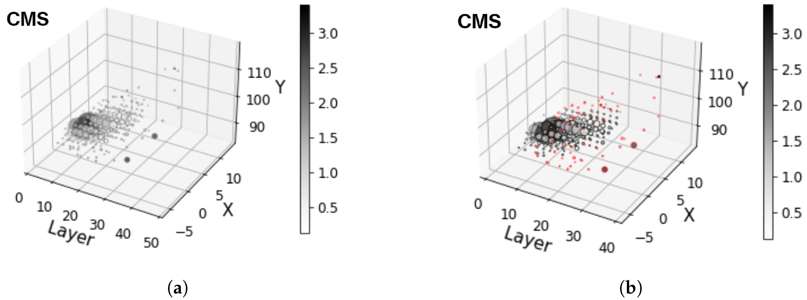
Passing through the calorimeter layers, the particles/decay products deposit energy in sensor cells grouped into trigger cells (TC). The trigger cells with the highest energies are grouped into 2D clusters within a single layer. Then, individual 2D clusters are connected into 3D ones, which gives complete 3D information about the shower (Figure 3a). If the targeted image size is smaller than an individual 2D cluster range, not all trigger cells participate in such image creation. It is shown in Figure 3b, where all TCs are bordered depending on whether they participate in image generation (black border) or not (red border).

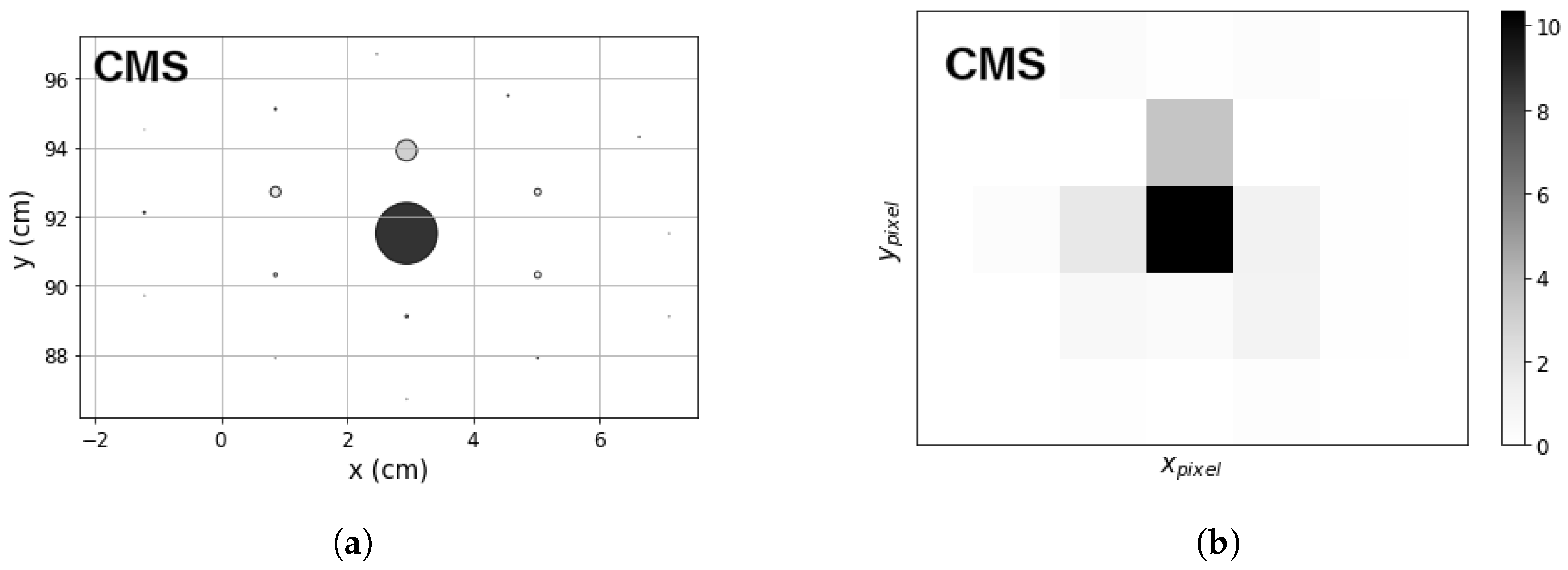
Subsequently, from the 3D cluster data obtained from CMSSW, virtual images are created by applying the following steps: the line between the center of mass of the 3D cluster and the center of the detector represents the deposition axis. The intersection point of the axis with each individual layer is the center of the region of interest (ROI) on that layer (Figure 4a). Afterward, the range along the coordinate axes is calculated according to the center depending on the target size of the ROI. Finally, a 2D histogram of 5 × 5 bins, with a bin size 2 × 2 cm² (adjusted to the size of the trigger cell), is applied to summarize all the energies (Figure 4b). The study [44] has shown that with a similar data set, window size enlargement does not significantly impact model accuracy.

As a result of the described image generation procedure, 3D images with a shape 5 × 5 × 36 are generated. The 5 × 5 parameter represents the window size, while the third value indicates the number of displayed layers (i.e., depth).

Since every second layer is used for triggering in the electromagnetic part of the calorimeter, it is described with 14 images, while the hadronic part consists of the remaining 22 layers, one for each layer. Figure 5 represents the longitudinal profile for EM (Figure 5a), PU (Figure 5b), and QCD showers (Figure 5c). It is clear that compared with EM showers (on average), PU and QCD start showering earlier, with a peak reached before layer 10 and a higher energy deposit in the hadronic part.

Observing the distribution of the total energy of EM clusters with PU and QCD clusters, shown in Figure 6, it is evident that EM clusters, on average, have significantly higher energy than background clusters.

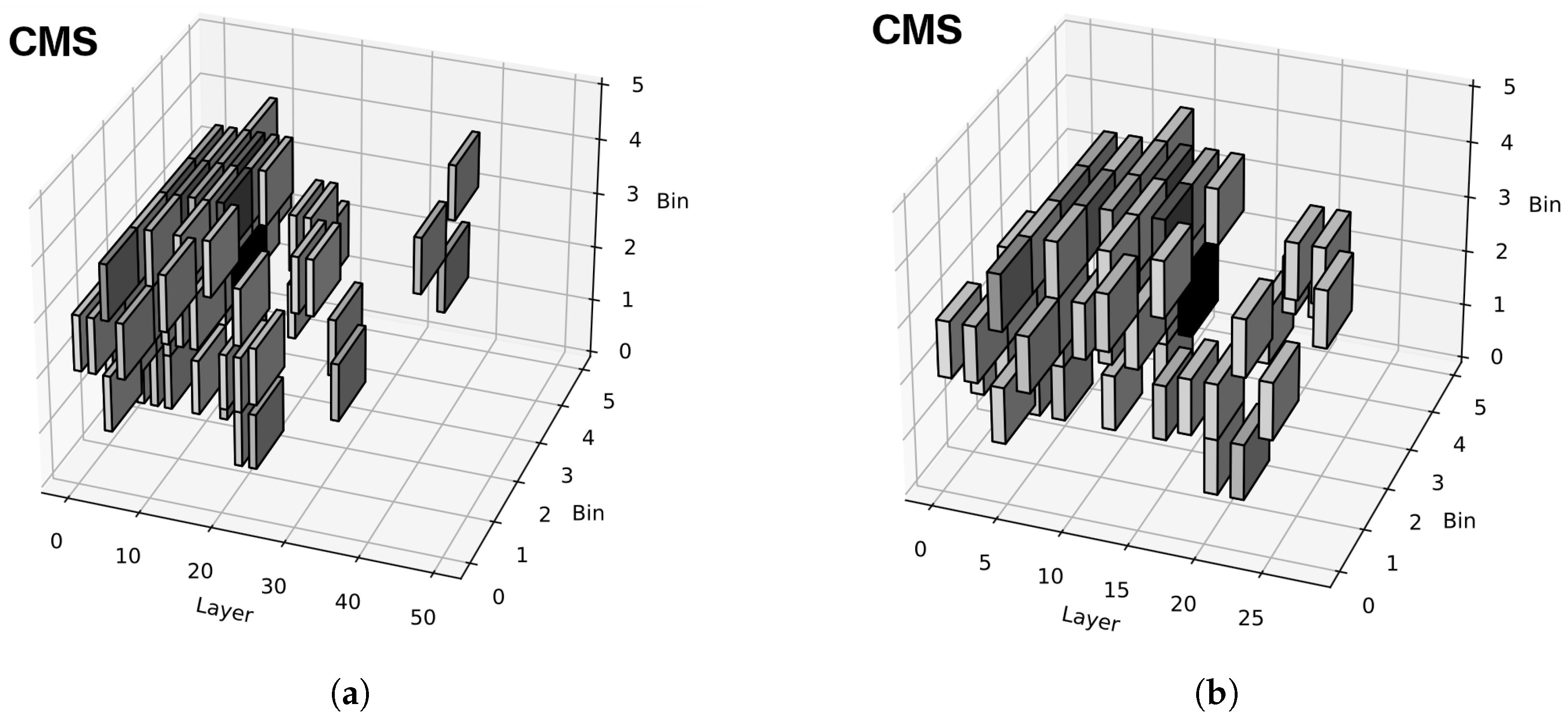
The models are tested on full HGCAL image (Figure 7a), but for some of the tested approaches, like a reduction in the longitudinal profile, the HGCAL image is split into CE-E and CE-H image parts. CE-E image has a shape 5 × 5 × 14 (Figure 7b) and shows only the electromagnetic part of the calorimeter, while CE-H image with a shape 5 × 5 × 22 represents the hadronic part.

3.1.4. Image Preprocessing

Pixel intensities can have large variations between different images; quite often, they span a few orders of magnitude. In addition, there are a significant number of outliers, especially in the PU data set. If left unaddressed, these data could potentially dominate the classification procedure (due to their larger scale) [45] or hinder the modeling/learning process [46]. Thus, we introduced a couple of carefully chosen pre-processing techniques to address this issue while ensuring data validity and accurate NN performance.

Feature normalization is applied to improve the numerical stability of model(s) and speed up the training process. In regard to outliers in a dataset, the straightforward procedure for handling outliers is to remove them from a dataset. But in our case study, outliers are the highest energy points, and deleting them would mean losing vital information. Some standard approaches in the presence of outliers are to use (quantile-based) capping [47] or robust scaler normalization [45].

Tests were performed with both techniques, and they showed similar results in terms of accuracy performance. However, capping proved simpler to implement and demonstrated better performance in terms of stability and resource utilization when applied to FPGAs. Thus, it was selected and applied only in some test cases, as is presented in more detail in Section 3.2.

The selection and quantization of input data are also considered to reduce the model’s memory footprint, enabling its implementation on FPGAs and the execution of event selection in the set time frame (<12 $\mu$s). Two types of data quantizers are created: linear, where the quantization levels are evenly distributed, and non-linear, where the relationship between the quantization levels is logarithmic.

3.2. Data Refinement

In addition to the data set containing complete HGCAL images, given in full precision, different ways of data refinement are considered. Although the size of the images is small (5 × 5), a high number of channels (HGCAL layers) results in a high number of pixels-features. Depending on the studied number of layers, it is 350 (for the CE-E part) or 900 for the complete HGCAL. Therefore, although the new detector structure enables analysis of a detailed collision image, the possibility of dimensionality reduction (the process of reducing the number of features) is examined. In the case where image data are observed, the number of pixels can be considered the number of features; each pixel represents one feature. Thus, the aim of the data refinement process, consisting of data selection and data quantization, is to reduce the quantity of data (i.e., data complexity) that the network needs to deal with to achieve lower inference time while retaining a similar performance level. This, in turn, is driven by the strict timing constraints of L1T.

Two main approaches in dealing with high-dimensional data are feature extraction (FE) and feature selection (FS). FE creates new features combining the existing ones, while FS identifies the relevant features and removes the redundant and irrelevant features. In [48], the authors review FE methods that reduce processing time while providing higher recognition accuracy. Although FE is the preferred approach in image processing, because of time and resource constraints, both approaches are used to scale down the dimensionality of the data without performance degradation. The experiment uses ad-hoc solutions suitable for our specific physically motivated classification problem. Considering the low computational time, two techniques are applied: filtering out the irrelevant pixel values (FS approach) and combining/summing particular layers (FE approach). Further reduction in resource consumption is achieved by data quantization. Data refinement is conducted in two steps: first, data selection, followed by data quantization. Particular techniques were chosen based on physics-based and logical-based reasoning, which is presented for each respective approach, while their applicability was determined through exhaustive testing.

3.2.1. Selection

In the first step, the selection is applied to full-precision data using one of the rules:

• Keep energies above the threshold.
  Here, a fixed threshold value of 0.1, 0.5, 1, 2 GeV is applied, all pt values greater than the threshold are kept, and others are set to 0. The smallest energy values are assumed to have minimal impact on determining if a cluster represents a signal or background. The reason behind the small values proposed for the thresholds is that TC energies are much smaller than cluster pt.
• Keep layer maximum (single sample per layer).
  With this approach, just the maximum value in each layer is kept, while other values are set to 0. This approach assumes that the highest pt deposits have a decisive role in shower classification.
• Capping.
  Data capping is a method in which the maximum value of a feature is set to a specific value. It is a standard technique to treat outliers and is often a necessary step in executing the model in FPGA. A preliminary test with models implemented in FPGA using hls4ml has shown a drop in the accuracy of even 10% in dealing with non-capped data (compared with QKeras model accuracy).
• Reduction in longitudinal profile.
  Similar to the approach presented in [49] where detector images consist of three subdetector channels: one each for CE-E, CE-H, and one for the reconstructed tracks, the following data refinement method is based on summing pt/pixels from particular detector layers. By summing the values of individual layers, it is possible to considerably reduce the image (channels) size, drastically decreasing the NN model’s size. Two different solutions are examined:
  • Considering the fact that EM shower leaves pt deposits mainly in the CE-E part of the HGCAL, all CE-H layers are projected in one plane, reducing the number of CE-H layers from 22 to 1. This approach is named E+Hf, and the same logic with the CE-H part is also applied in the next solution.
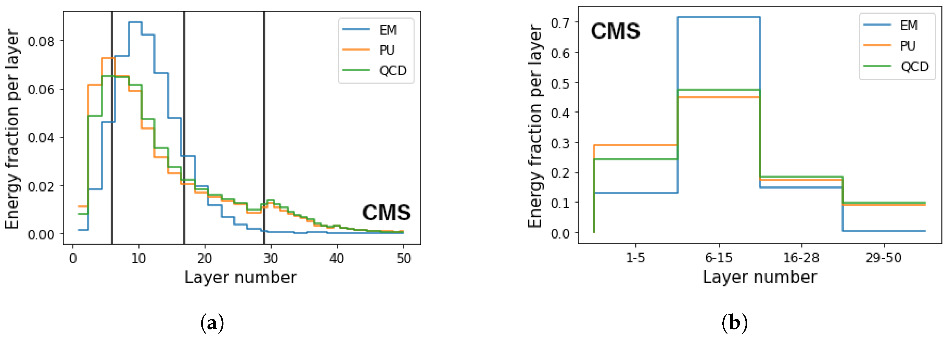
  • Here, the fact that EM starts showering in the earlier detector layers and reaches the peak between layers 10 and 15 is used. The CE-E is divided into three parts: layers 1–5, where the EM shower starts; layers 6–15, where the most pt is deposited; and layers 16–28, shown in Figure 8a. Each part is summed (Figure 8b), resulting in 3 5 × 5 CE-E images, and the CE-H part is reduced, creating a 5 × 5 CE-H image. This approach is referred to as 3Ef+Hf.

3.2.2. Quantization

The reason behind the data quantization is it enables additional limitations of resource usage. Data are quantized in three ways using custom quantizers:

• Selection bit(s).
  Here, all data values that have passed the previously applied selection steps have a value of 1. Using this approach, FPGA implementation requires just 1 bit for each value in the input data layer presentation.
• Uniform quantizer.
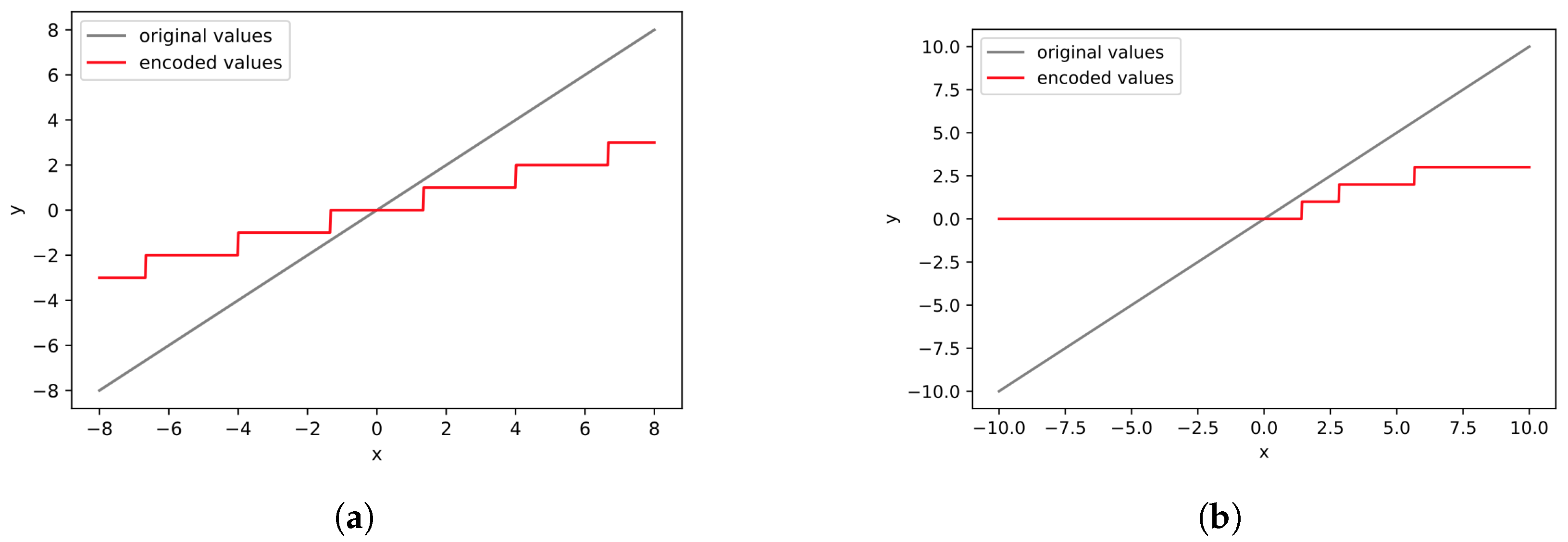
  Min-max normalization is applied on capped data, multiplied by $2^n-1$, where n is a chosen number of bit width. The result is rounded to the nearest integer. The proposed quantizer function is presented in Figure 9a.

  $$Q\left(x\right)=round(\frac{x-min}{max-min}·(2^n-1))$$

  (1)
• Non-uniform quantizer. The quantizer is defined as follows

  $$Q\left(x\right)=\left\{\begin{array}{cc}round\left(lo{g}_2\left(x\right)\right),\hfill & \mathrm{if}x>0\hfill \\ -2,\hfill & \mathrm{otherwise}\hfill \end{array}\right.$$

  (2)
  The next step is to rescale data (using a min-max scaler), so it does not contain negative values. The non-uniform quantizer function is presented in Figure 9b.

An overview of data refinement methods described in this section is given in

Table 1. Data refinement methods.

Refinement Methods
Selection	Quantization
Keep energies above the threshold	Selection bit
Keep layer maximum	Uniform quantizer
Capping	Non-uniform quantizer
Reduction of longitudinal profile

.

3.3. Model Architectures

Already in 1989, Cybanko [50] proved that standard multilayer feedforward networks could approximate any continuous function of n real variables to any desired accuracy. The same year, Hornik et al. [51] showed that multilayer feedforward networks with as few as one hidden layer are universal approximators. In the last decade, state-of-the-art models like CoAtNets, ResNet, EfficientNet, YOLOv5, and many others have been developed. They achieve excellent results, but the high computational complexity of neural network-based classifiers and their requirements on the resources do not allow their usage in L1T, where power consumption is limited, as well as budget on available devices.

3.3.1. Model Size

The first strategy to reduce computational complexity is limiting the network size in the sense of several layers and neurons while taking care of model performance. In more complex computer vision tasks, it would lead to significantly worse performance. Still, it is shown in [44,52] that deep multilayer perceptron (MLP) with just three layers can be successfully used in EM shower/PU classification. Unlike in the previous approaches, the new classification cases are added, with background represented as QCD events and a mixed background scenario with both QCD and neutrino PU events.

Two simple NN models are considered: MLP and CNN, but because of space constraints, just the last classification case for both models is analyzed in detail since it includes both types of backgrounds. The hyperparameter optimization software framework Optuna [53] is used to determine the models’ structure. Optuna uses a tree-structured Parzen estimator sampler, a Bayesian optimization technique that models the search space. It uses the history of previously evaluated hyperparameter configurations to sample the following ones.

For the CNN, the search space contains 6–16 kernels for the Conv2D layer and 8–18 nodes in the following 1–2 dense layers, so far resulting in 1452 possible network combinations. For the MLP, the search space contains 2–3 layers, each with 4–16 nodes, generating 2366 combinations. The proposed activation functions for intermediate layers for both models are ReLu and sigmoid, while the output layer uses softmax for the activation function. The search space also contains optimizers, namely, Adam, RMSprop, and SGD, each with a range of learning rates, greatly increasing the number of possible combinations in the search space to 8712 for CNN and 14,196 for MLP. The HGCAL images, which are in 3D tensor format, require reformatting to serve as suitable inputs for MLP; i.e., to ensure compatibility with the MLP architecture, the tensor needs to be reshaped into a 1-dimensional vector.

When more architectures with similar accuracies are highly ranked, the one that minimizes the number of trainable parameters is chosen.

3.3.2. Model Quantization

The second strategy to reduce memory footprint and computational complexity is model quantization, a process of model transformation into an equivalent representation but using parameters and computations at a lower precision. According to [54], the usage of low-precision fixed integer value representation has the potential to reduce the memory footprint and latency by a factor of 16×. Despite being fast and very easy to use, the post-training quantization approach is not an option because it suffers from significant degradation in model accuracy in case of precision lower than 8 bits [55].

Please note that any quantization (and, in some cases, data reduction, as introduced previously) results in loss of data accuracy, i.e., quantization error. However, since we aim to implement a selection algorithm for L1T and not a (final) data analysis algorithm, our work was not affected by this issue in a traditional manner. We aimed to reduce data complexity to the point where it was just about sufficient to differentiate said data from other signal types (with high accuracy) while reducing their impact on NN memory and resource footprints (within defined timing and resource constraints). In this process, we worked with data copies and were thus not limited by data accuracy in the final analysis since if the proposed algorithm flagged an event as being of interest (i.e., EM shower), the complete set of data (with full precision) would be sent for storage via other channels for later analysis. This should be kept in mind when interpreting the proposed (aggressive) quantization.

The QKeras library enables quantization-aware training using a simple replacement for Keras layers, greatly simplifying the quantization process. QKeras allows heterogeneous quantization: it is possible to use different quantization levels and different quantized activation functions on each layer. The concept of a straight-through estimator presented in [56] is used; hence, the forward pass applies the quantization functions, and the backward pass adopts the quantization as the identity function to make the gradient differentiable [57]. After exhaustive research, it was decided to use the quantizer $quantized\_bits$ defined as follows

$$2^{int-b+1}clip(round(x\ast 2^{b-int-1}),-2^{b-1},2^{b-1}-1)$$

(3)

for weights and kernels, where x = input, b = number of bits for the quantization, $int$ = how many bits are to the left of the decimal point.

$Quantized\_relu$ is chosen as a quantized replacement for the ReLu activation function, used in the inner layers of models.

3.4. Evaluation

This section presents the metrics used to demonstrate the impact of quantization, model selection, and data refinement techniques on model performance.

3.4.1. Standard Metrics

Essential evaluation metrics usually used to illustrate the performance of the classifiers are:

• accuracy (ACC), percentage of correct classifications, calculated as

  $$ACC=\frac{TP+TN}{TP+TN+FP+FN}$$

  (4)
• sensitivity, recall, or true positive rate (TPR)

  $$TPR=\frac{TP}{TP+FN}$$

  (5)
• specificity, or true negative rate (TNR)

  $$TNR=\frac{TN}{TN+FP}$$

  (6)
• false negative rate (FNR)

  $$FNR=\frac{FN}{FN+TP}=1-TPR$$

  (7)
• false positive rate (FPR)

  $$FPR=\frac{FP}{FP+TN}=1-TNR$$

  (8)
• F1 score

  $$F1=2\frac{PPV\ast TPR}{PPV+TPR}.$$

  (9)

where $TP$ stands for the number of correctly predicted positive classes, $TN$ is the number of correctly predicted negative classes, $FP$ is the number of samples incorrectly predicted as positive classes, and finally, $FN$ is the number of samples incorrectly predicted as negative classes. In the case of class imbalance, accuracy is not a good metric. Instead, the $F1$ score is defined as the harmonic mean of precision (PPV, where $PPV=\frac{TP}{TP+FP}$) and recall, designed to work well on imbalanced data.

Also, it is a standard technique for summarizing classifier performance (for a balanced dataset) to produce a receiver operating characteristic curve (ROC), which represents the false positive rate (FPR) versus the true positive rate (TPR), and the corresponding area under the curve (AUC) is calculated. We note that when dealing with imbalanced datasets, it is more appropriate to use a precision–recall curve instead of an ROC curve. The former curve summarizes the trade-off between the true-positive rate and the positive predictive value for a predictive model using different probability thresholds. In the HEP, it is common to interpret the ROC curve in terms of signal efficiency (the true-positive rate) vs. background rejection (true negative rate). Also, physicists are often interested in other metrics, like signal efficiency at some fixed level of background rejection.

There exist many metrics for classification models, but for particle detector triggers, it is essential to detect as many interesting events as possible in addition to accuracy. Therefore, the trigger algorithm should operate at a very low FNR. On the other hand, low FPR ensures staying within the available trigger bandwidth but does not impact the success of the analysis.

3.4.2. Classification Threshold Adjustment

Depending on the application, binary classification often needs to optimize specific metrics, such as the minimization of FNR or FPR (the same as maximizing TNR or TPR). Sometimes, the default threshold (0.5) may not represent an optimal interpretation of the predicted probabilities. It is the case when the predicted probabilities are not calibrated, which is a known problem for modern neural networks [58]. Also, when the cost of one type of misclassification is more important, changing the default decision threshold is one way to handle it. According to [59], misclassifying an actual positive example into a negative is often more expensive than an actual negative example into a positive. Thresholding is a cost-sensitive meta-learning method described in [60], based on the selection of the probability that minimizes the total misclassification cost on the training instances as the threshold for predicting testing instances. Therefore, when interpreting the predictions of a model, sometimes there is a need to change the default decision threshold of 0.5. If TPR and TNR have the same importance for the L1 trigger, one way of calculating the cut-off is using Youden’s J statistic ([61]), defined as follows:

$$J=Sensitivity+Specificity-1,$$

(10)

or simplified:

$$J=TPR-FPR.$$

(11)

Youden’s index is often used in combination with ROC curve analysis. The index is calculated for all points of an ROC curve, and the optimal threshold with the largest J value is chosen. If both metrics, FNR and FPR, are not equally important, using the trial and error method helps find the threshold to lower the targeted metric.

3.5. Baseline Particle Classification Methods

As baseline methods to be compared to NN-based approaches, the simple cut-off method and Random Forest (RF) were applied. Please note that these two methods are usually employed in HEP for triggering purposes, making their comparison with the proposed approach of interest. However, when making such comparisons and interpreting the obtained results, it should be kept in mind that there is a significant difference in technology, spatial resolution, and data characteristics between the HGCAL under development (for which the proposed approach is intended) and the existing one for which the previously mentioned triggering algorithms are used.

3.5.1. Cut-Off

Considering the fact that average EM cluster pt is much higher than PU or QCD cluster pt as shown in Figure 6, the simplest approach to particle classification is to apply linear selection criteria: (pt) cut-off value can be used to accept or reject clusters as EM, as it is likely that the low pt cluster is background. The test is performed with two cut-off values: the first is the maximum PU (QCD) cluster pt, and the second is the third quartile PU (QCD) cluster pt value.

3.5.2. Random Forest

Another baseline method is RF, a supervised ML algorithm that combines the output of multiple decision trees to reach a single result. Together with BDT, it is often used in particle classification, as shown in [62,63]. Both RF and BDT usually use data sets containing well-known physical parameters as features. In our tests, because of the time constraints needed for L1T selection, the same input applied for NN models was used: raw detector data—that is, HGCAL images.

RF consists of a large number of decision trees that operate as an ensemble. Each individual tree in the RF declares a class prediction, and the class with the most votes becomes the model’s prediction. In the RF learning process, there are two major layers of randomness. The first random component is that RF uses a random (bootstrapped) sample of the original training data set for each individual decision tree. As a result, in the vast majority of cases, the training sets for the trees are different from one another, which reduces the correlation between trees and improves the generalization of the predictions making RF more robust to overfitting [64]. Another layer of randomness is in the (random) selection of the features considered at each node. The method itself is introduced by Leo Breiman ([65]), and a detailed method analysis is available in [66]. RF’s simple usage and flexibility, together with the possibility to handle classification and regression problems, have contributed to its widespread usage. It is considered to be one of the best off-the-shelf-learning algorithms, requiring almost no tuning, although it enables fine control over the model that is learned. However, it does have some disadvantages compared to other classification methods (like decision trees), which should be kept in mind when interpreting its results and applicability: its models are more complex and harder to interpret (although feature importance can be readily obtained), and due to the stochastic nature of tree building, the structure of the trained model is unpredictable, requiring more time and system resources to train and run.

An open-source machine learning library for the Python programming language named scikit-learn [67] is used for testing RF classifiers as it provides a robust implementation combining both algorithmic and code optimization. To improve the accuracy of the RF classifier for particular situations, there are parameters that may be tuned. The grid search is used for performing hyper-parameter optimization, employing the next hyperparameter search space:

• max_features: maximum number of features random forest considers splitting a node, with available values ’auto’, ’sqrt’, ’log2’. The default value is ’auto’.
• n-estimators: the number of trees in the forest, with values 100, 200, 300. Increasing this hyperparameter generally improves the performance of the model. The drawback is it also increases the computational cost of training and predicting. The default value is 100.
• max_depth: maximum number of levels in each decision tree, using values 8, 16, 20. The default value is none, which means that nodes are expanded until all leaves are pure or until all leaves contain fewer than 2 samples.

An additional parameter, criterion, which measures the quality of the split, with values ’gini’ and ’entropy’, is added to the search space too, and the loss function, which is optimizing the accuracy.

3.6. hls4ml

Recently, in 2018, Duarte et al. [68] presented hls4ml, a compiler that translates ML models into register transfer level for FPGAs using the high-level synthesis (HLS) tool. hls4ml enables models’ firmware feasibility without comprehensive Verilog/VHDL experience, thus accelerating the development cycle. Although there are many similar tools available [69], this tool was selected for this study since it is an open-source tool that supports the usage of QKeras and Xilinx development chains and Xilinx FPGA boards (which are targeted FPGA boards for the new detector). Please note that the selection of a translator tool is not critical for this study and is more related to convenience. The obtained results and conclusions should hold for other similar tools, with the only foreseeable difference lying in the deployment stage (i.e., the results in Section 4.5).

The models described in this study use Vivado (2020.1) for HLS synthesis with a Xilinx Kintex UltraScale FPGA (part number xcvu13p-fhgb2104-2-e) [70] as the target device, with the synthesis clock frequency set to 200 MHz. To achieve as low as possible latency while maintaining accuracy, different settings are considered depending on the benchmark model. In the FPGA, hls4ml operates with fixed-point arithmetic. By adjusting the fixed-point data type and using profiling tools, it is possible to lower resource consumption.

The hls4ml profiling tool helps to decide appropriate model precision. Without profiling, low global precision settings that help to reduce the FPGA resource usage of a model may result in a loss of model performance if chosen inappropriately. Another hls4ml feature that helps to optimize an NN is the possibility of determining the parallelization of the calculations in each layer. It is performed by configuring the parameter reuse factor, which determines the number of times a multiplier is used to carry out a computation. It is clear that a fully parallelized process results in low latency but requires more resources; respectively, latency and required resources are inversely proportional. After setting the specified parameters, Vivado HLS is used to synthesize the model.

4. Results and Discussion

The following section presents the structure of NN used in the experiment and explains the results of the model and data quantization and selection methods described in the previous section. Please note that although the presented results were obtained from simulated data (which can be considered a limitation of the current study), due to the physics fidelity of the data generated by the simulator (as discussed in Section 3.1), we believe that the conclusions drawn can be transferred to real data with no or minimal NN re-training and adjustment.

4.1. Model Architectures

Here, the architecture of used CNN and MLP models is presented, followed by the model quantization results.

4.1.1. Base NN Models

The optimization results for the hidden layers of CNN and MLP models for each of the classification cases are shown in

Table 2. The results of model structure optimization for CNN and MLP for each classification case. The table describes just hidden layers.

Case/Model	CNN	MLP
EM vs. PU	conv1 layer: 11 kernels dense1 layer: 12 nodes	dense1 layer: 5 nodes dense2 layer: 13 nodes
EM vs. QCD	conv1 layer: 12 kernels dense1 layer: 10 nodes	ense1 layer: 4 nodes dense2 layer: 15 nodes
EM vs. MIX	conv1 layer: 6 kernels dense1 layer: 12 nodes dense2 layer: 13 nodes	dense1 layer: 8 nodes dense2 layer: 13 nodes

. For example, the CNN model for EM vs. PU classification contains a convolutional layer with 11 3 × 3 kernels followed by one dense layer with 12 nodes. It can be noticed that the optimizer gives quite a similar NN structure for MLP in all classification tasks, while the suggested CNN in EM vs. MIX is somewhat bigger; it has an additional dense layer, which is expected because the classification problem is more complex.

The activation functions are the same in all cases; the inner layers use ReLu, and classification is performed using softmax. For both models, the loss function is the binary cross-entropy, and optimization is conducted using the Adam algorithm, with a learning rate obtained by the optimizer and a batch size of 128. The learning rate values determined by the optimizer are in the range of 0.009 to 0.07, depending on the model and classification case. Early stopping is implemented if no progress is seen beyond ten epochs. Early stopping is a form of regularization that reduces model complexity and prevents overfitting [71].

Both the training and testing sets contain balanced samples of the classes in all the classification tasks. There are a total of 36,000 samples in each classification task, consisting of 18,000 EM samples and 18,000 background samples (either PU or QCD). Out of these, 15,300 samples of each type were used for training and validation, and 2700 were used for testing. The first group of tests was conducted on the full data set without any normalization, selection, or quantization. Input images represent the full HGCAL profile, that is, all 36 layers.

The results of baseline NN methods for different types of EM vs. background classification are shown: for PU in

Table 3. The results for the base CNN and MLP model for EM vs. PU.

Model	acc	prec	rec	f1	AUC	fpr	fnr
CNN	0.9861	0.9899	0.9822	0.9861	0.9951	0.0100	0.01781
MLP	0.9830	0.9891	0.9767	0.9829	0.9920	0.0107	0.0233

, for QCD in

Table 4. The results for the base CNN and MLP model for EM vs. QCD.

Model	acc	prec	rec	f1	AUC	fpr	fnr
CNN	0.9698	0.9756	0.9637	0.9696	0.9914	0.0241	0.0363
MLP	0.9639	0.9665	0.9611	0.9638	0.9884	0.0333	0.0389

, and for mixed background in

Table 5. The results for the base CNN and MLP model for EM vs. MIX.

Model	acc	prec	rec	f1	AUC	fpr	fnr
CNN	0.9731	0.9758	0.9704	0.9731	0.9899	0.0241	0.0296
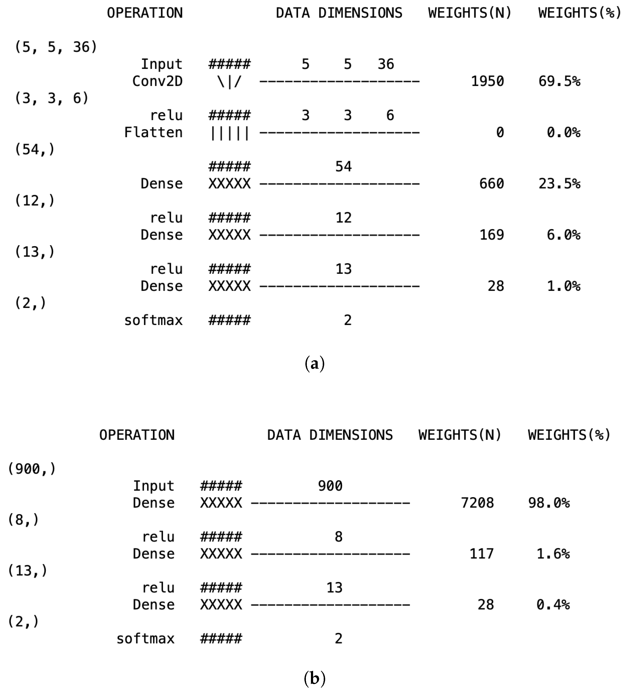
MLP	0.9689	0.9665	0.9715	0.9690	0.9893	0.0337	0.0285

. Architectures of the developed networks are presented in Figure 10.

It can be noticed that in all cases, CNN gives slightly better accuracy than MLP. Both models are better at classifying between EM and neutrino PU clusters than between EM and QCD jets. The EM vs. MIX classifier, as expected, is somewhat better than EM vs. QCD, and worse than EM vs. PU. In the rest of the paper, the focus is put on EM vs. MIX classification problem. The models are minimized, making them suitable for FPGA implementation and playing an important role in L1 triggering. At the same time, the methods described in the previous section are used to improve accuracy and minimize FNR.

4.1.2. Model Analysis

In this subsection, three critical aspects of model performance are examined: model robustness, error analysis, and the interpretation of model decisions.

It should be noted that simple robustness analysis was performed utilizing artificially introduced offsets in energy distribution profiles in regard to the layer in which particular energy appears. The NN models demonstrated good robustness without any changes in accuracy for offsets up to three layers (about 10% of ECAL size), while offsets of four or more layers resulted in an accuracy drop, especially in MLP. Additionally, in [72], we showed that the same family of NNs can cope with a change in the type of data being used; i.e., it was shown that models pre-trained on electron EM showers (which we used in our experiments) can successfully classify events containing photon EM showers. We believe all of this information demonstrates the robustness of the proposed approach.

Furthermore, the error analysis conducted in this study identified some potential limitations. Our findings suggest that the model struggles to differentiate between two scenarios due to the complex nature of the data. Specifically, the NNs may encounter difficulties in accurately predicting outcomes for low-energy EM showers that start appearing in earlier layers than usual. Additionally, EM instances wherein hadronic deposits are higher than usual also pose challenges to the model. The use of low-level features, such as HGCAL images and energy deposits, has its limitations when dealing with these specific scenarios.

To enable the interpretability of the presented models, the SHAP (Shapley additive explanations) [73,74] framework was used. It allows one to understand the contribution of each feature to a model’s output, making the decision-making process clearer. SHAP values provide an explicit indication of feature importance, making it easier to comprehend a model’s operation. Both MLP and CNN models were investigated utilizing SHAP, providing insights into the key factors influencing model predictions. After conducting an extensive literature review and examining the SHAP tool’s documentation, no examples of its application for 3D image classification were found. As a result, we had to make certain adjustments to the tool to accommodate our data, which limited the use of some of the (standard) SHAP functionalities. Despite this, useful insights into the operation of the models were gained, identifying the most important features for accurate predictions. A summary of the key findings is given below:

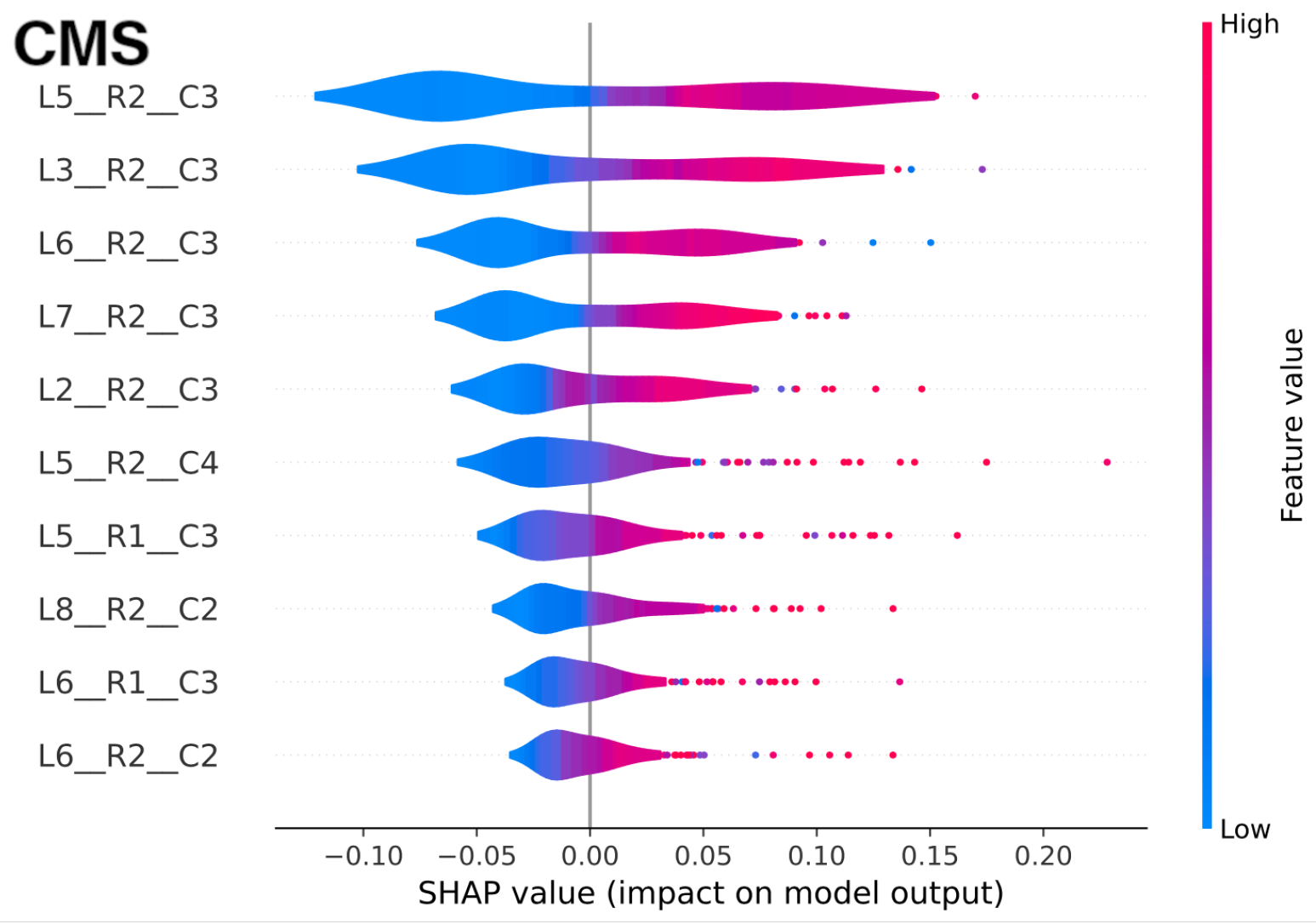
• To utilize MLP for EM classification based on raw detector data, the 3D HGCAL image is flattened. This essentially means that the 3D image is transformed into a 1D array of values, where each value represents a pixel. To be precise, there are 900 pixels in the flattened version of the image, and these pixels serve as the features for the classification task. To ensure absolute clarity in the different pixel positions, the feature name is always displayed in the following format: layer_row_column. It is worth noting that the position of each pixel in a particular channel or layer is not as significant as the layer itself. The summary plot given in Figure 11 provides an overview of the most impactful features of a model. It ranks these features according to their effect on the model’s predictions. The x-axis represents the SHAP value, which is a measure that quantifies the influence of a feature on a specific prediction. The y-axis displays the features, while the plot also shows the distribution of SHAP values for each feature. The color of the plot indicates the value of the feature, ordered from low to high. Upon closer examination of the diagram, it is noticeable that the features or pixel positions that have the greatest impact on the prediction are mostly between layers 5 and 10 (Figure 11 shows just the first top-ranked features). These are the layers in which the PU and QCD reach peak energy deposition (for reference, please see Figure 5).
• Similar to the MLP model, the CNN architecture undergoes a feature importance analysis using SHAP values. However, the SHAP documentation does not provide a way in which to visualize the 3D regions with the highest influence on model decisions. Therefore, we created a custom visualization that follows standard SHAP rules. This visualization produces a figure wherein red pixels indicate the features that cause the model to predict that an HGCAL image corresponds to an EM shower, while blue pixels indicate the features that push the model away from predicting that an image belongs to the EM class. Figure 12 gives a visualization of an example of SHAP local interpretation. Essentially, local interpretation involves calculating the SHAP values for each feature for a specific instance, providing insight into which features were most important for that decision. It is noticeable that most of the red areas are within the layers where the EM showers have the most energy deposits (for reference, please see Figure 5). This indicates that the model pays significant attention to these areas when predicting an EM shower.

4.1.3. Model Quantization

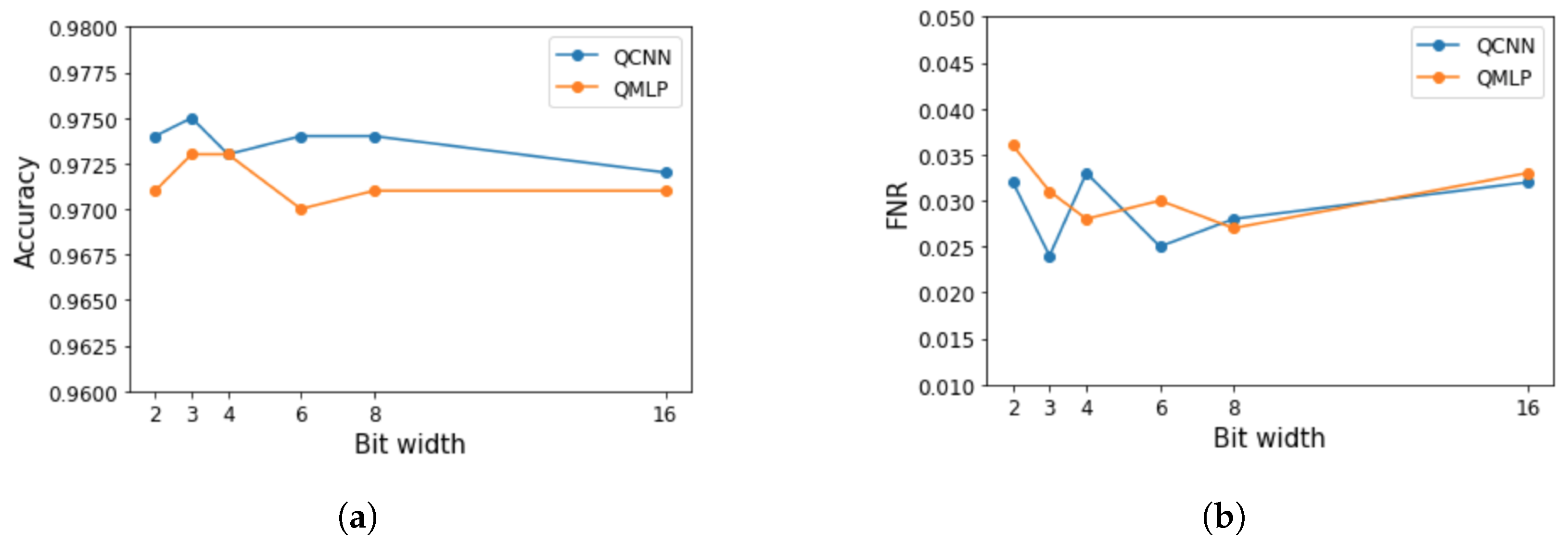
To examine the effect of weight/bias/kernel quantization level on model accuracy, tests are conducted iterating over the number of bits for the quantization in the range from 2 to 16, and there is no significant difference in achieved results. The comparison of accuracy and FNR for different quantization levels given in Figure 13 shows that accuracy is very similar for all quantization levels, while FNR varies more. Therefore, given that the goal is model minimization in the sense of memory footprint and processing requirements, aggressive 2-bit quantization of model weights/biases/kernels is chosen to be applied for model quantization, even if FNR is higher than, for example, for 6-bit quantized models.

In the rest of the paper 2-bit quantized CNN is referred to as QCNN, and accordingly, the quantized 2-bit version of MLP is named QMLP.

The performance of the 2-bit quantized version of CNN and MLP is summarized in

Table 6. The results for the 2-bit quantized CNN and MLP models.

Model	acc	prec	rec	f1	AUC	fpr	fnr
QCNN	0.9737	0.9790	0.9681	0.9736	0.9875	0.0207	0.0319
QMLP	0.9713	0.9782	0.9641	0.9711	0.9812	0.0215	0.0359

. It is evident that the quantized models have the same discrimination power as the baseline architectures. Considering memory and processing limited devices on which the trigger algorithms will be implemented, from now on, the study is conducted just on quantized models. Comparing QCNN with QMLP, it is evident that both models provide very similar results. All metrics are slightly higher for QCNNs, confirming that convolutional layers ensure better performance in computer vision problems.

4.2. Baseline Particle Classification Methods

4.2.1. Cut-Off

The data set contains 18,000 samples for each of the three types of clusters, and 3628 of them, or 20.16%, are low-pt EM clusters, EM clusters with pt lower than maximum PU cluster pt that would be lost, using these criteria. Compared with QCD clusters, there are 8159, or 45.33% low pt clusters. In the case of the third quartile cut-off value, 45 EM clusters (0.25 %) are lost in the case of the EM/PU classification and 87 (0.48 %) in the EM/QCD classification. On the other side, using a cut-off value lower than the maximum PU (QCD) cluster pt, the number of wrongly classified PU (QCD) clusters grows rapidly, resulting in unnecessary storage of useless data.

Therefore, simply accepting/rejecting clusters based on cluster pt value is not an acceptable option for the L1T selection method.

4.2.2. Random Forest

Using the same metrics as for NN models, the RF classifier with default settings gives the results presented in

Table 7. The results of random forest classifier.

Settings	acc	prec	rec	f1	AUC	fpr	fnr
default	0.9693	0.9731	0.9652	0.9691	0.9693	0.0267	0.0348
optimized	0.9694	0.9735	0.9652	0.9693	0.9694	0.0263	0.0348

.

The hyperparameter optimization gives the next combination of tuned hyperparameters: criterion: ’gini’, max_depth: 40, max_features: ’auto’, n_estimators: 200. The achieved metrics are almost the same as those obtained with the predefined settings, which are shown in Table 7. Even though the achieved accuracy is similar to the NN model’s case, both FNR and FPR are slightly higher. The next attempt is to run a grid search to optimize the recall score, but with no improvement (maximizing recall, FNR is minimized).

4.3. Classification Threshold Adjustment

Two popular evaluation metrics to estimate the model performance, accuracy, and AUC are for QCNN and QMLP models above 97%, indicating good performance. Following the procedure described in Section 3.4.2, for QCNN, the largest J statistic (0.947) is achieved using a threshold value of 0.939913, and for QMLP, the maximum J value (0.944) is for a threshold of 0.851953. However, this threshold value selection resulted in better FPR results but increased FNR value for both models, as seen in

Table 8. The results for the QCNN and QMLP (gray background) with different threshold values.

Threshold	acc	prec	rec	f1	AUC	fpr	fnr
0.1	0.9698	0.9604	0.9800	0.9701	0.9875	0.0404	0.0200
0.1	0.9689	0.9678	0.9700	0.9689	0.9812	0.0322	0.0300
0.5	0.9737	0.9790	0.9681	0.9736	0.9875	0.0207	0.0319
0.5	0.9713	0.9782	0.9641	0.9711	0.9812	0.0215	0.0359
0.939913	0.9744	0.9845	0.9641	0.9742	0.9875	0.0152	0.0359
0.851953	0.9717	0.9826	0.9604	0.9713	0.9812	0.0170	0.0396

.

On the other side, with the trial and error approach, using a threshold value of 0.1, FNR decreases to 0.02 for QCNN and to 0.03 for QMLP. Although the differences in achieved FNR are not high, it is important to remember that the volume of the data set on which the model is intended to be used is very high, and even small differences in percent result in high absolute values. For example, for QCNN, the difference between the best achieved FNR and FNR obtained for the default threshold is 0.0119 (1.19%). Applied to a data set with just 1,000,000 samples, it ends with 11,900 additionally recognized EM clusters, and any of them could have a significant role in some new physical discovery. A comparison of results obtained using different thresholds is given in Table 8.

Even though the obtained FNR (3.19% for QCNN and 3.59% for QMLP) and FPR (2.07% for QCNN and 2.15% for QMLP) are not high for the base quantized models with default threshold, using the thresholding technique they can be further optimized. It should be noted that the number of FPs increases by changing the threshold to decrease the FNs.

It can be noticed there is no big difference in moving the threshold based on J-statistics or looking for minimization of FPR and FNR difference, but depending on needs, it is clear that it is possible to optimize targeted costs by choosing the appropriate threshold.

4.4. Data Refinement

This section describes the effect of different data refinement methods on NN model performance.

4.4.1. Selection

• Keep energies above the threshold.
  Before processing, in the training data set for the 5 × 5 × 36 sample, there are just 11.37% non-zero values. Using different threshold values, for the described method, the percent of non-zero values decreases: for threshold value 0.1 GeV to 5.99%, for 0.5 GeV to 1.67%, for 1 GeV to 1,01%, and finally for threshold value 2 GeV to 0.6%. As is visible in

  Table 9. The QCNN and QMLP (gray background) results with different thresholds applied on energy/pixel values.

  Threshold (GeV)	acc	prec	rec	f1	AUC	fpr	fnr
  0.1	0.9722	0.9800	0.9641	0.9720	0.9844	0.0196	0.0359
  0.1	0.9674	0.9647	0.9704	0.9675	0.9835	0.0356	0.0296
  0.5	0.9706	0.9711	0.9700	0.9705	0.9851	0.0289	0.0300
  0.5	0.9676	0.9685	0.9667	0.9676	0.9823	0.0315	0.0333
  1	0.9693	0.9774	0.9607	0.9690	0.9826	0.0222	0.0393
  1	0.9667	0.9684	0.9648	0.9666	0.9851	0.0315	0.0352
  2	0.9578	0.9870	0.9278	0.9565	0.9657	0.0122	0.0722
  2	0.9556	0.9858	0.9244	0.9541	0.9643	0.0133	0.0756

  , as the threshold value increases, accuracy slightly drops, and there is an increase in FNR value for the threshold values higher than 0.5. Therefore, forthcoming tests are not carried out for those threshold values.
• Keep layer maximum (single sample per layer).
  The models where just one value per image layer is kept show no drop in classification precision compared with base quantized versions, according to results shown in

  Table 10. The results for the keep layer maximum approach for QCNN and QMLP.

  Model	acc	prec	rec	f1	AUC	fpr	fnr
  QCNN	0.9706	0.9725	0.9685	0.9705	0.9834	0.0274	0.0315
  QMLP	0.9689	0.9713	0.9663	0.9688	0.9814	0.0285	0.0337

  .
• Capping.
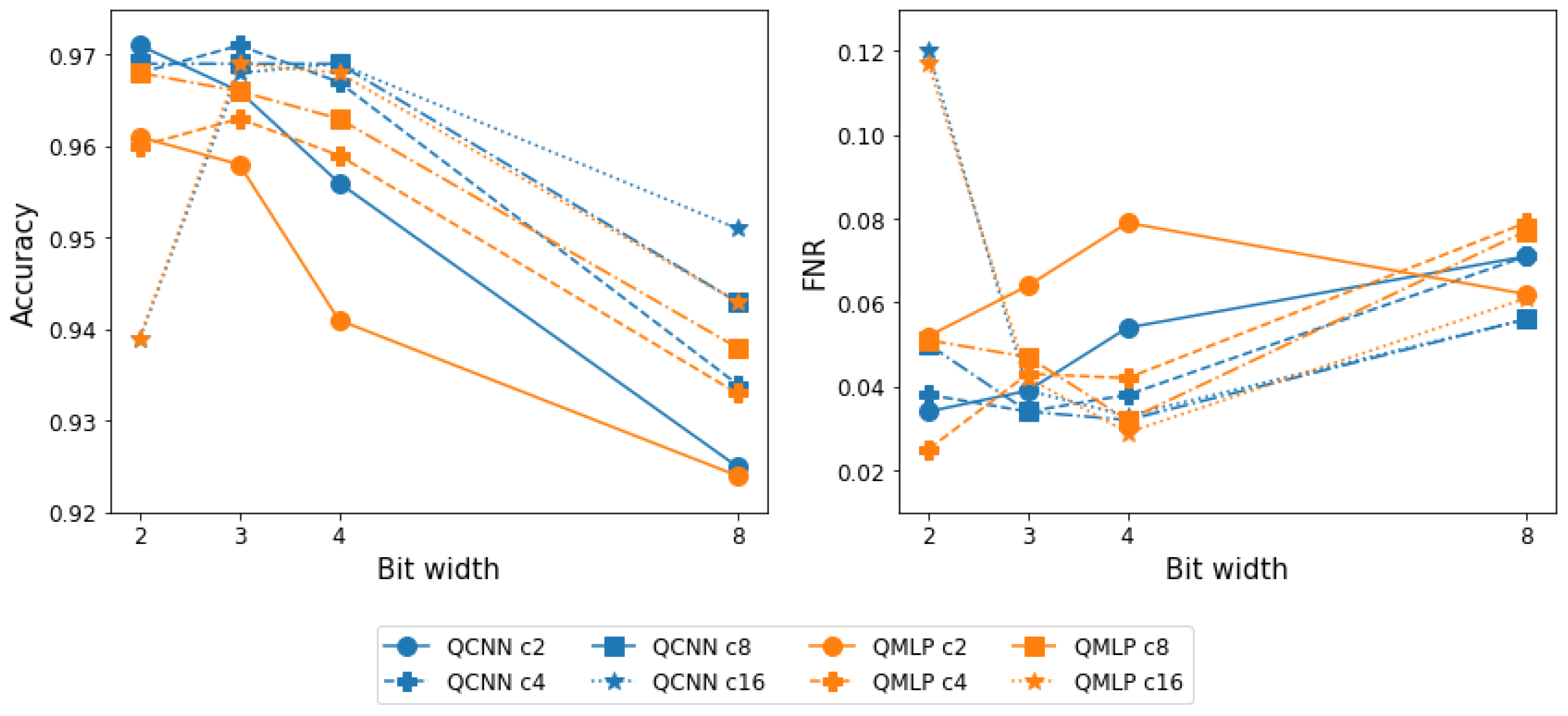
  Data capping is performed by using different values (2, 4, 8, 16). For QMLP, there is no notable difference in metrics, but for QCNN, there is an improvement in FNR for all capping values (

  Table 11. The results for the QCNN and QMLP (gray background) with different capping values.

  c_value	acc	prec	rec	f1	AUC	fpr	fnr
  2	0.9739	0.9723	0.9756	0.9739	0.9856	0.0278	0.0244
  2	0.9678	0.9688	0.9667	0.9677	0.9811	0.0311	0.0333
  4	0.9741	0.9737	0.9744	0.9741	0.9860	0.0263	0.0256
  4	0.9704	0.9757	0.9648	0.9702	0.9836	0.0241	0.0352
  8	0.9731	0.9674	0.9793	0.9733	0.9871	0.0330	0.0207
  8	0.9713	0.9775	0.9648	0.9711	0.9811	0.0222	0.0352
  16	0.9744	0.9741	0.9748	0.9745	0.9861	0.0259	0.0252
  16	0.9702	0.9725	0.9678	0.9701	0.9824	0.0274	0.0322

  ), no matter which capping value is chosen. The impact of the applied capping value on the model’s accuracy is shown in Figure 14a and on FPR in Figure 14b.
• Reduction in longitudinal profile.
  The complete HGCAL image contains 5 × 5 × 36 = 900 pixels per image, resulting in 2807 parameters for QCNN (respectively 7353 for QMLP). Here, QCNN is used as a classifier. As a result of reducing the longitudinal profile following procedures described in Section 4, the number of model parameters is drastically decreased. The described solutions are examined and results are shown in

  Table 12. The results for the reduction in longitudinal profile approach for QCNN.

  Model	acc	prec	rec	f1	AUC	fpr	fnr
  E+Hf	0.9728	0.9691	0.9767	0.9729	0.9855	0.0311	0.0233
  3Ef+Hf	0.9702	0.9686	0.9719	0.9702	0.9883	0.0315	0.0281

  :
  • The QCNN model using a full HGCAL image has 2807 parameters, and with this approach (E+Hf), the number of parameters is reduced to 1673.
  • This approach (3Eh+Hf) replaces the full HGCAL image (5 × 5 × 36) with a 5 × 5 × 4 image, decreasing the NN parameter numbers to 1079.

As is clear from the above description, in approaches 1, 2, and 3, the HGCAL layer structure image is retained. The global picture of particle decay is kept but simplified, emphasizing the importance of high pt points above very small pt deposits. Theoretically, instead of sending the complete image, just the position and value kept after the applied selection could be sent, notably cutting back the number of parameters in the NN’s input layer. Using approach 4, the number of layers can be drastically decreased, ultimately significantly reducing the number of neural network parameters.

4.4.2. Data Quantization

In this section, different data quantization approaches are presented.

• Selection bit(s).
  The combination of data thresholding and selection bit method would reduce the amount of data needed for acceptance/rejection decision even more. According to performance metrics shown in

  Table 13. The results of the selection bit method applied after thresholding, for the QCNN and QMLP (gray background) model.

  Threshold (GeV)	acc	prec	rec	f1	AUC	fpr	fnr
  0.1	0.9611	0.9615	0.9607	0.9611	0.9832	0.0385	0.0393
  0.1	0.9302	0.9029	0.9641	0.9325	0.9752	0.1037	0.0359
  0.5	0.9659	0.9611	0.9711	0.9661	0.9784	0.0393	0.0289
  0.5	0.9676	0.9664	0.9689	0.9676	0.9839	0.0337	0.0311

  , for a threshold value 0.1, there is a drop in accuracy for both models, while a threshold value of 0.5 followed by selection bits method for QCNN gives results comparable to those achieved with complete full-precision data.
• Uniform quantizer.
  A mandatory step to use uniform quantization is capping. Otherwise, as there is a wide range of values used for image presentation, most of them would become 0 after applied quantization. Figure 15 shows model accuracies and FNR depending on the capping value applied before uniform quantization.
  According to Figure 13, for a lower number of chosen bit widths (2–4) for data quantization, both QCNN and QMLP achieve better results for accuracy and FNR. Capping values 2 and 4 give better results than 8 and 16; hence 4 is chosen to be applied as the capping value whenever uniform quantization is used, and results are given in

  Table 14. Uniform quantizer with different quantization levels, QCNN and QMLP (gray background) models.

  Bit Width	acc	prec	rec	f1	AUC	fpr	fnr
  2	0.9676	0.9727	0.9622	0.9674	0.9844	0.0270	0.0378
  2	0.9598	0.9461	0.9752	0.9604	0.9825	0.0556	0.0248
  3	0.9711	0.9757	0.9663	0.9710	0.9870	0.0241	0.0337
  3	0.9633	0.9689	0.9574	0.9631	0.9816	0.0307	0.0426
  4	0.9672	0.9723	0.9619	0.9670	0.9789	0.0274	0.0381
  4	0.9593	0.9606	0.9578	0.9592	0.9791	0.0393	0.0422
  8	0.9339	0.9383	0.9289	0.9336	0.9573	0.0611	0.0711
  8	0.9330	0.9438	0.9207	0.9321	0.9635	0.0548	0.0793

  .
  According to Table 14, models with 2 and 3 input data bit width outperform models with wider data precision.
• Non-uniform quantizer.
  The models based on non-uniformly quantized data with results in

  Table 15. Non uniform quantizer.

  Model	acc	prec	rec	f1	AUC	fpr	fnr
  QCNN	0.9685	0.9766	0.9600	0.9682	0.9860	0.0230	0.0400
  QMLP	0.9678	0.9730	0.9622	0.9676	0.9834	0.0267	0.0378

  show somewhat lower performances than models based on 2-bit uniformly quantized input.

4.5. hls4ml

Considering model accuracy and FNR, along with model size (in terms of the number of parameters and precision of input data), the first model implemented in hls4ml is QCNN with full precision data, with capping value 8, referred to as QCNN_FP. It is compared with QCNN with 2-bit quantized input data, from now on referred to as QCNN_U2. The last model implemented in hls4ml is QMLP with 2-bit quantized input data, named QMLP_U2E. It must be emphasized that because of some restrictions in Vivado/hls4ml on the number of parameters, the input data are images covering just the CE-E part of the HGCAL. The FPGA implementation results for each of the models are reported in

Table 16. The results of FPGA implementation for different models.

Model	Time [ns]	Interval [Cycles]	Latency [$\mathsf{\mu }$s] (Cycles)	FF # (%)	LUT # (%)
QCNN_FP	4.374	30	0.170 (34)	19,655 (2.27)	63,874 (14.79)
QCNN_U2	4.37	30	0.170 (34)	20,594 (2.38)	63,261 (14.64)
QMLP_U2E	4.320	5	0.085 (17)	1134 (0.13)	43,401 (10.05)

. It is important to bring attention to the fact that, in this case, (hls4ml) models are not optimized in the sense that the precision is adjusted by layers. They use the precision defined at the model level, with settings necessary to preserve the accuracy of the QKeras model. It is clear that all models satisfy the required latency constraint (<12 $\mu$s). FPGA resource usage metrics show flip-flop (FF) employment in all cases is under 2.5%, and lookup table (LUT) utilization is under 15%. For all models, the number of used digital signal processors (DSP) is two, which, compared to available DSPs (3072), makes 0.065%.

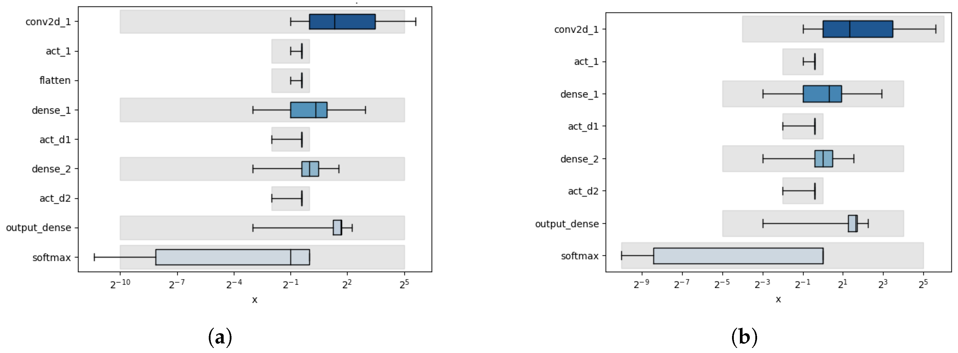
Using low precision settings can help reduce the FPGA resource usage of a model but may result in loss of model performance if chosen inappropriately. In addition to setting the model precision, hls4ml allows per-layer optimization. The profiling tools in hls4ml help to decide the appropriate model/layer precision. Each layer in the QNN is evaluated using the given test data, and the distribution of values is shown with a box and whisker diagram. The grey-shaded boxes show the range, which can be represented with the used hls4ml configuration settings.

When the test is performed with QCNN_U2, using default hls4ml precision <16, 6>, there is a gap between QKeras (0.968148) and hls4ml (0.9409259) accuracy. The profiling tool has shown that first-layer output precision has to be extended from the default (Figure 16a). With models’ extended precision <18, 8>, accuracy is improved (0.9679629).

To show the effect of input data quantization together with the possibility of per-layer optimization, the model QCNN_U2 is implemented in three different ways: first using default settings, second optimizing the hidden layer precision, and finally optimizing the input layer precision, as shown in Figure 16b.

Afterward, the resource usage for those three cases is compared, which is shown in

Table 17. The results of different types of optimizations for the QCNN_U2 model.

Settings	FF #	FF %	LUT #	LUT %
default	20,594	2.38	63,261	14.64
hidden layer precision adjusted	19,670	2.28	61,387	14.21
input + hidden layer precision adjusted	13,008	1.51	57,884	13.40

. With per-layer optimization for model inner layers, FF # goes down 4.5% (from 20,594 to 19,670) and LUT # 3% (from 63,261 to 61,387). Compared with the model where the input layer is also adjusted, the savings in FF # are 36.8% and 8.5% in LUT #. The other metrics (time, interval, and latency) are the same in all three cases, corresponding to the default model implementation, shown in Table 16.

5. Conclusions and Future Work

This paper describes a neural network (NN) model for classifying electromagnetic (EM) showers from the mixed background made of pile-up (PU) and quantum chromodynamics (QCD) jets at level 1 trigger within a given time limit of a few $\mu$s. Recent advances have made it possible to adjust the NN models to limitations caused by the targeted hardware, field programmable gate arrays (FPGAs).

The first tests are carried out with a data set containing ideal signal (EM) images; in the data simulation step, it was chosen to generate EM showers without PU. The NN classifiers distinguishing between idealistic EM showers and PU achieve 99% accuracy. The EM shower with included PU is generated to get closer to a more realistic situation. As there is a big difference in average EM and PU cluster pt, which simplifies the classification process, another type of particle, QCD jets, is also added to background samples. Simple convolutional neural network and multi-layer perceptron models with signal/background classification accuracy between 96 and 99% and false negative rate (FNR) between 2 and 4%, depending on the background case, are developed. The achieved results could eventually be improved by adding physical features to input data, but it would be difficult to incorporate into level 1 trigger latency requirements. The rest of the paper considers the EM versus mixed background, one-vs-all classification problem. Using the QKeras quantization library, NN models are aggressively quantized, representing the weights and activations with 2 bits, reducing computational and memory costs (in inference time) with accuracy degradation of less than 1%. Further, different approaches to data refinement are presented. The methods that affect the range of input data, like capping, using appropriate values, can significantly lower FPR (for a quantized convolutional neural network with capping value 8, by 34%). Image size reduction methods also decrease the FNR value, lowering the number of NN parameters. The quantization methods, uniform quantization, and selection bit approach achieve performances comparable to a base model, with a large reduction in the precision required for the data storage. As shown, the presented data refinement methods have enabled further reduction in the model resource consumption. Using the hls4ml library, model examples are converted into the firmware to be implemented on FPGA. All implemented models can be executed with a latency lower than 1 $\mu$s and flip-flop and lookup table utilization under 2.5% and 15%, respectively. Using variants of implementation of the proposed quantized convolutional neural network, it is shown that model and data quantization enable additional savings of resources when implementing the model in FPGA: the number of used flip-flops is reduced by 36.8% and the number of lookup tables by 8.5%. To address the limitations caused by HGCAL images of particles that have a showering pattern that differs from what is expected, future efforts will focus on introducing new features, possibly including high-level ones, or exploring more advanced model architectures that can better capture the subtleties of the data. Another possible future research avenue is to search for an efficient method with which to exploit the sparsity of calorimeter images.