Author Contributions
Conceptualization, M.S. and B.C.; methodology, M.S.; software, M.S.; validation, M.S.; formal analysis, B.C.; investigation, M.S.; resources, B.C.; writing—original draft preparation, M.S. and B.C.; writing—review and editing, B.C.; visualization, M.S. and B.C.; supervision, B.C.; project administration, B.C.; funding acquisition, B.C. All authors have read and agreed to the published version of the manuscript.
Figure 1.
A schematic representation of the process of feeding the coefficients of a polynomial into an Artificial Neural Network (ANN), which then yields an approximation for each root of Equation (
1).
Figure 1.
A schematic representation of the process of feeding the coefficients of a polynomial into an Artificial Neural Network (ANN), which then yields an approximation for each root of Equation (
1).
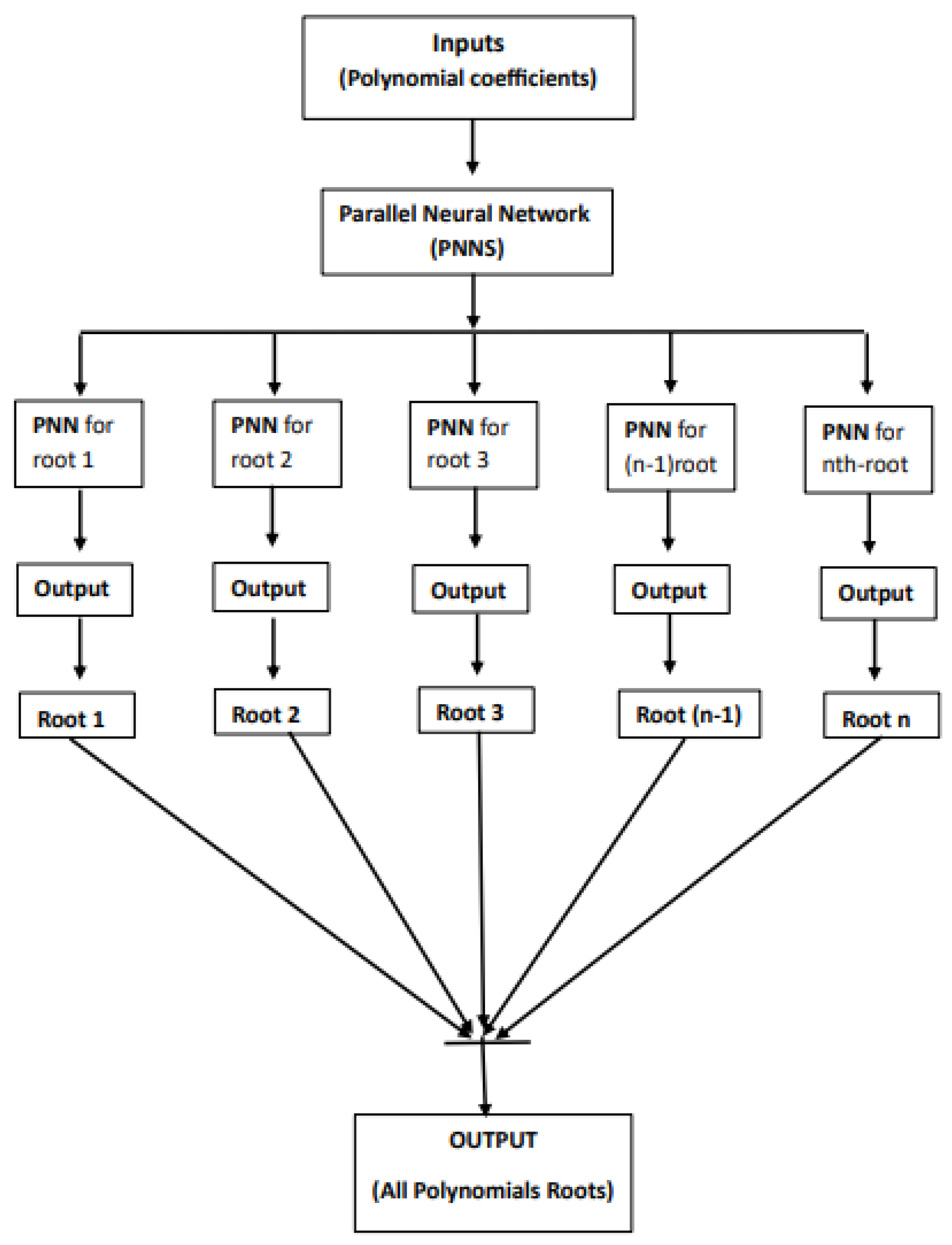
Figure 2.
A schematic representation of the process of feeding the coefficients of a polynomial into an Parallel Neural Network (PNNS), which then yields an approximation for each root of Equation (
1).
Figure 2.
A schematic representation of the process of feeding the coefficients of a polynomial into an Parallel Neural Network (PNNS), which then yields an approximation for each root of Equation (
1).
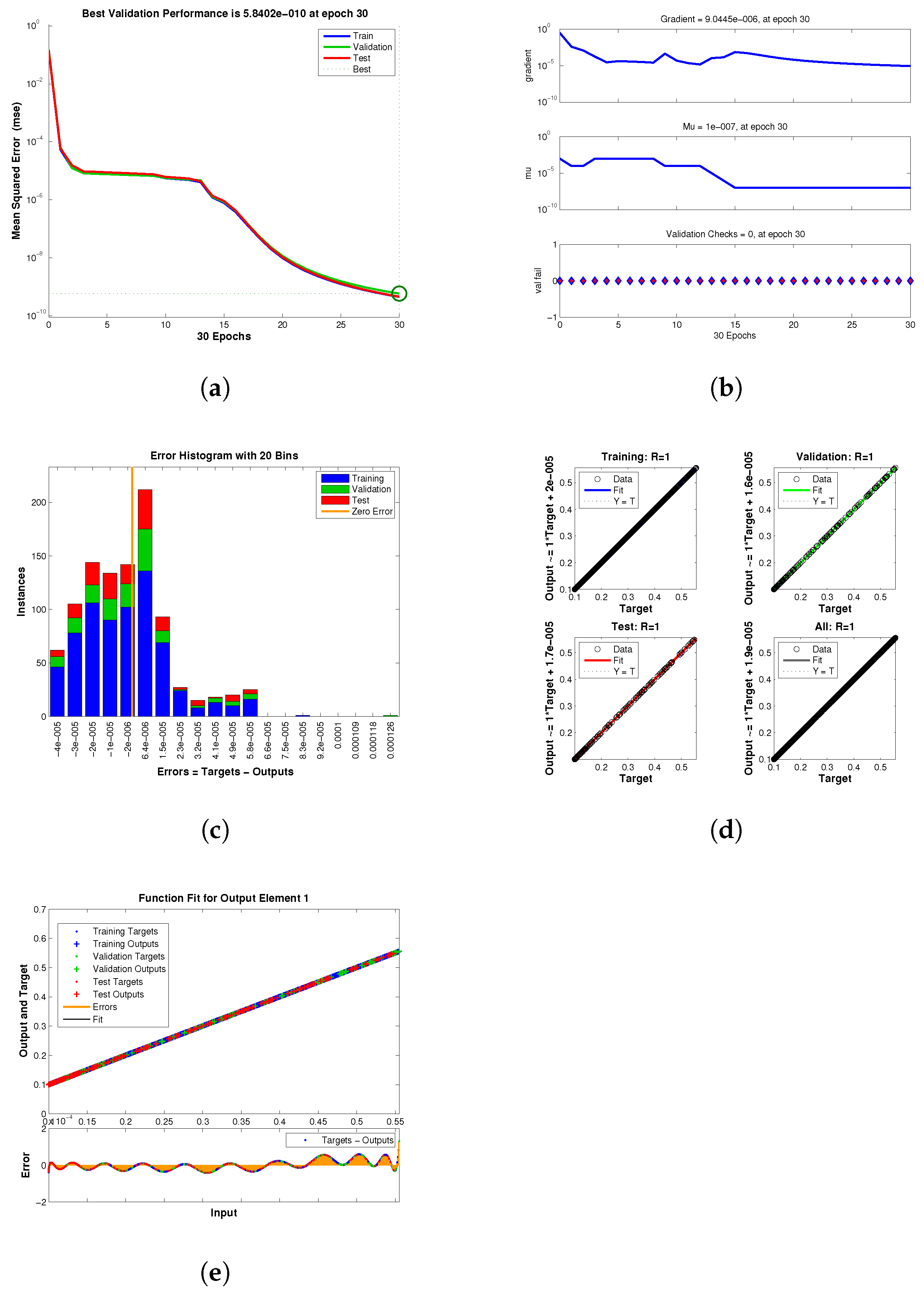
Figure 3.
(a–e) Error histogram of neural network for engineering application 1 (b) Transition statistics curve of neural network for engineering application 1 (c) Mean square error curve of neural network for engineering application 1 (d) Regression curve of neural network for engineering application 1 (e) Fitness curve of neural network for engineering application 1. (a) The neural network’s error histogram. (b) The neural network’s transition statistics curve. (c) The neural network’s mean square error curve. (d) The neural network’s regression curve. (e) The neural network’s fitness curve.
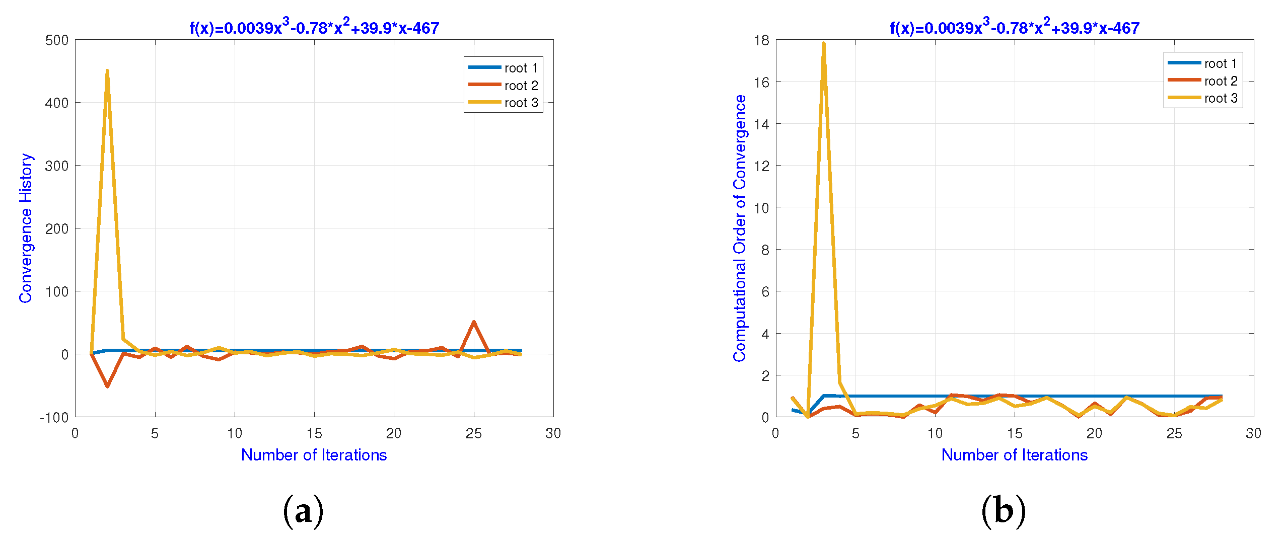
Figure 4.
(a,b) The convergence path of the approximated roots for engineering application 1 using a neural network, (b) the neural network-based computational order of convergence of the approximate roots for engineering application 1. (a) The neural network’s convergence path. (b) The computational order of convergence.
Figure 5.
(a–f) Using the neural network’s output as input, the local computational order of convergence of required 24 iterations to converge (b) using the neural network’s output as input, the local computational order of convergence of required 30 iterations (c) using the neural network’s output as input, the local computational order of convergence of required 25 iterations (d) using the neural network’s output as input, the local computational order of convergence of required 22 iterations (e) using the neural network’s output as input, the local computational order of convergence of required 19 iterations (e) using the neural network’s output as input, the local computational order of convergence of required 16 iterations to converge. (a) Local computing order of convergence. (b) Local computing order of convergence. (c) Local computing order of convergence. (d) Local computing order of convergence. (e) Local computing order of convergence. (f) Local computing order of convergence, for solving biomedical engineering application 1.

Figure 6.
(a–e) Error histogram of neural network for engineering application 2 (b) Transition statistics curve of neural network for engineering application 2 (c) Mean square error curve of neural network for engineering application 2 (d) Regression curve of neural network for engineering application 2 (e) Fitness curve of neural network for engineering application 2. (a) The neural network’s error histogram. (b) The neural network’s transition statistics curve. (c) The neural network’s mean square error curve. (d) The neural network’s regression curve. (e) The neural network’s fitness curve.
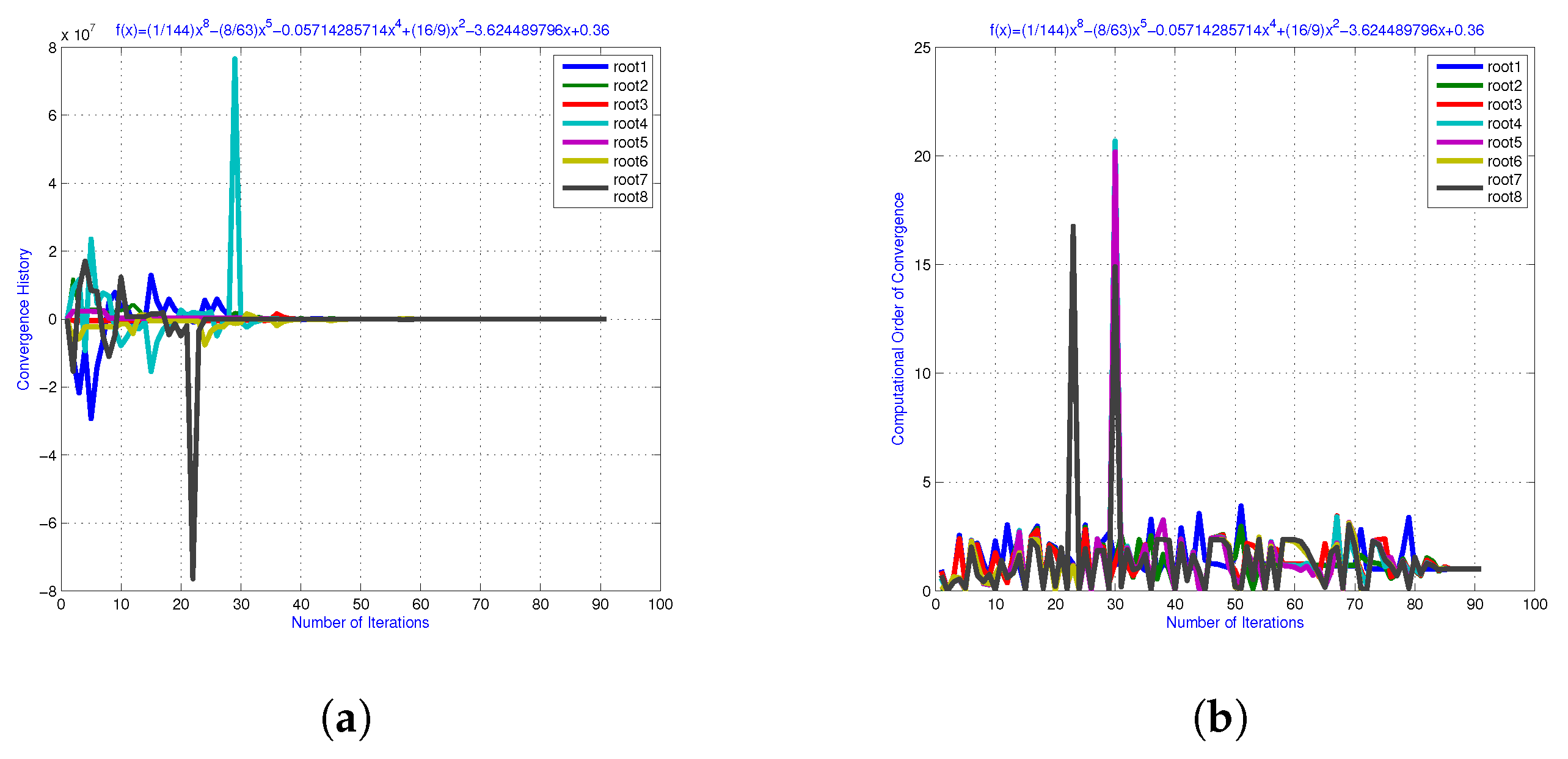
Figure 7.
(a,b) The convergence path of the approximated roots for engineering application 2 using a neural network (b) the neural network-based computational order of convergence of the approximate roots for engineering application 2. (a) The neural network’s convergence path. (b) The computational order of convergence.
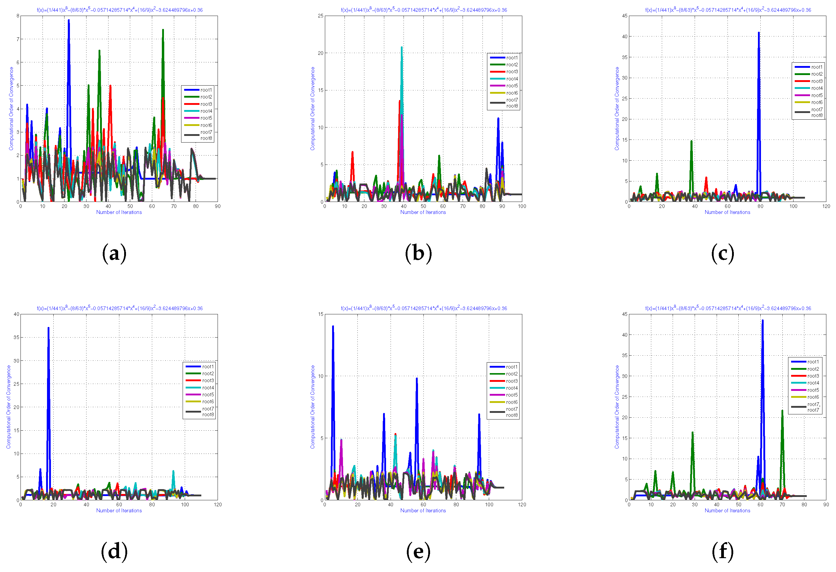
Figure 8.
(a–f) Using the neural network’s output as input, the local computational order of convergence of required 80 iterations to converge (b) Using the neural network’s output as input, the local computational order of convergence of required 90 iterations (c) using the neural network’s output as input, the local computational order of convergence of required 119 iterations (d) using the neural network’s output as input, the local computational order of convergence of required 19 iterations (e) Using the neural network’s output as input, the local computational order of convergence of required 115 iterations (e) using the neural network’s output as input, the local computational order of convergence of required 80 iterations to converge. (a) Local computing order of convergence. (b) Local computing order of convergence. (c) Local computing order of convergence. (d) Local computing order of convergence. (e) Local computing order of convergence. (f) Local computing order of convergence.

Table 1.
Error analysis and roots approximation using the method with on engineering application 1.
Table 1.
Error analysis and roots approximation using the method with on engineering application 1.
|
|---|
| q | | | | | | | | | |
| | | | − | | i | − | | i |
| | | | | | | | i | |
| | | 2.1 | | | | | − | − |
| − | − | + | − | | | | | |
| | | | | | | | | |
| | | | | | | | | |
| | | | | | | | | |
| | | | | | | | | |
| | | | | | | | | |
Table 2.
Max-Error for the method using .
Table 2.
Max-Error for the method using .
| | | |
|---|
| | | |
| | | |
| | | |
| | | |
| | | |
| | | |
| | | |
| | | |
| | | |
Table 3.
Number of iterations for using .
Table 3.
Number of iterations for using .
| It- | It- | It- |
|---|
| 16 | 16 | 16 |
| 16 | 16 | 16 |
| 18 | 18 | 18 |
| 20 | 20 | 20 |
| 26 | 26 | 26 |
| 27 | 27 | 27 |
| 28 | 28 | 28 |
| 85 | 85 | 85 |
| 100 | 100 | 100 |
Table 4.
CPU-time for the method using .
Table 4.
CPU-time for the method using .
| CT- | CT- | CT- |
|---|
| 1.94215 | 1.9415 | 1.8451 |
| 2.14561 | 2.54165 | 2.14554 |
| 3.0124 | 3.00124 | 3.01245 |
| 3.12415 | 3.24156 | 3.21451 |
| 3.54126 | 3.84561 | 3.98451 |
| 4.00121 | 4.00125 | 4.00165 |
| 4.01234 | 4.12013 | 4.18745 |
| 5.01242 | 5.12415 | 5.1421 |
| 5.12455 | 5.14215 | 6.1425 |
Table 5.
Error analysis and roots approximation using the method with on engneering application 1.
Table 5.
Error analysis and roots approximation using the method with on engneering application 1.
|
|---|
| q | | | | | | | | | |
| | − | | − | | | − | | |
| | | | | | | | | |
| | | | | | | | − | − |
| − | − | | − | − | | | | |
| | | | | | | | | |
| | | | | | | | | |
| | | | | | | | | |
| | | | | | | | | |
| | | | | | | | | |
Table 6.
Max-Error for the method using .
Table 6.
Max-Error for the method using .
| | | |
|---|
| | | |
| | | |
| | | |
| | | |
| | | |
| | | |
| | | |
| | | |
| | | |
Table 7.
Number of iterations of using .
Table 7.
Number of iterations of using .
| It- | It- | It- | It- |
|---|
| 5 | 5 | 5 | 5 |
| 5 | 5 | 5 | 5 |
| 7 | 7 | 7 | 7 |
| 8 | 8 | 8 | 8 |
| 8 | 8 | 8 | 8 |
| 11 | 11 | 11 | 11 |
| 14 | 14 | 14 | 14 |
| 17 | 17 | 17 | 17 |
| 22 | 22 | 22 | 22 |
Table 8.
CPU-time using .
Table 8.
CPU-time using .
| CT- | CT- | CT- |
|---|
| 0.04215 | 0.0415 | 0.0451 |
| 0.14061 | 0.54105 | 0.14004 |
| 2.0124 | 2.00124 | 2.01245 |
| 2.12415 | 2.3056 | 2.21451 |
| 3.54126 | 3.84561 | 3.98451 |
| 3.10111 | 3.00125 | 3.4126 |
| 4.21234 | 4.15123 | 4.18745 |
| 4.01242 | 4.12425 | 4.64201 |
| 4.12455 | 4.13125 | 4.14112 |
Table 9.
Error outcomes using neural networks on application 1.
Table 9.
Error outcomes using neural networks on application 1.
| Method | | | | |
|---|
| | | | 3.4714 |
| | | | |
| | | | |
| | | | |
| | | | |
| | | | |
| | | | |
Table 10.
Improvement in convergence rate using neural network outcomes as input for the parallel root finding scheme.
Table 10.
Improvement in convergence rate using neural network outcomes as input for the parallel root finding scheme.
| Method | | | | |
|---|
| | | | |
| | | | |
| | | | |
| | | | |
| | | | |
| | | | |
| | | | |
Table 11.
Overall results of q-analogies-based neural network outcomes for accurate initial guesses.
Table 11.
Overall results of q-analogies-based neural network outcomes for accurate initial guesses.
| Method | | | | | |
|---|
| | | | | |
| | | | | |
| | | | | |
| | | | | |
| | | | | |
| | | | | |
| | | | | |
Table 12.
Error analysis and roots approximation using the method with on engineering application 2.
Table 12.
Error analysis and roots approximation using the method with on engineering application 2.
|
|---|
| q | | | | | | | | | |
| | | | | | | | | |
| | | | | | | | | |
| | | | | | | | | |
| − | − | − | − | − | − | − | − | − |
| − | − | − | − | − | − | − | − | − |
| −2.2-1.94i | − | − | − | − | − | −2.2-1.94i | − | − |
| − | − | − | − | − | − | − | − | − |
| | | | | | | | | |
| | | | | | | | | |
| | | | | | | | | |
| | | | | | | | | |
| | | | | | | | | |
| | | | | | | | | |
| | | | | | | | | |
| | | | | | | | | |
| | | | | | | | | |
| | | | | | | | | |
Table 13.
Max-Error for the method using on engineering application 2.
Table 13.
Max-Error for the method using on engineering application 2.
| | | | | | | | |
|---|
| | | | | | | | |
| | | | | | | | |
| | | | | | | | |
| | | | | | | | |
| | | | | | | | |
| | | | | | | | |
| | | | | | | | |
| | | | | | | | |
| | | | | | | | |
Table 14.
Number of iterations for the method using .
Table 14.
Number of iterations for the method using .
| It- | It- | It- | It- | It- | It- | It- | It- |
|---|
| 63 | 63 | 63 | 63 | 63 | 63 | 63 | 63 |
| 63 | 63 | 63 | 63 | 63 | 63 | 63 | 63 |
| 77 | 77 | 77 | 77 | 77 | 77 | 77 | 77 |
| 79 | 79 | 79 | 79 | 79 | 79 | 79 | 79 |
| 85 | 85 | 85 | 85 | 85 | 85 | 85 | 85 |
| 87 | 87 | 87 | 87 | 87 | 87 | 87 | 87 |
| 91 | 91 | 91 | 91 | 91 | 91 | 91 | 91 |
| 97 | 97 | 97 | 97 | 97 | 97 | 97 | 97 |
| 99 | 99 | 99 | 99 | 99 | 99 | 99 | 99 |
Table 15.
CPU-time method using .
Table 15.
CPU-time method using .
| CT- | CT- | CT- | CT- | CT- | CT- | CT- | CT- |
|---|
| 6.3325 | 6.1424 | 7.1241 | 7.2148 | 6.2145 | 6.3251 | 6.2145 | 6.2525 |
| 6.3214 | 6.2145 | 6.9856 | 6.3298 | 6.8547 | 63214 | 7.2145 | 6.3214 |
| 7.3652 | 7.1456 | 7.32145 | 7.3214 | 7.1452 | 7.3652 | 7.1245 | 7.1426 |
| 7.2145 | 7.3652 | 7.1245 | 7.3652 | 7.1254 | 7.6521 | 7.3256 | 7.1254 |
| 7.36541 | 7.98654 | 7.6935 | 7.96523 | 7.3214 | 7.69321 | 7.8546 | 8.2156 |
| 8.36521 | 8.96542 | 8.32154 | 8.36542 | 8.36954 | 8.21453 | 8.6352 | 8.9658 |
| 8.65418 | 8.6954 | 8.6598 | 8.74566 | 8.3654 | 9.6532 | 8.3214 | 9.3654 |
| 9.45178 | 9.1024 | 10.2541 | 8.7454 | 9.6542 | 9.8745 | 9.4157 | 9.6542 |
| 9.1241 | 9.84512 | 9.41524 | 8.5412 | 9.35412 | 9.8754 | 9.4157 | 9.4571 |
Table 16.
Error analysis and roots approximation using the method with on engineering application 2.
Table 16.
Error analysis and roots approximation using the method with on engineering application 2.
|
|---|
| q | | | | | | | | | |
| | | | | | | | | |
| | | | | | | | | |
| | | | | | | | | |
| − | − | − | − | − | − | − | − | − |
| − | − | − | − | − | − | − | − | − |
| − | − | − | − | − | − | − | − | − |
| − | − | − | − | − | − | − | − | − |
| | | | | | | | | |
| | | | | | | | | |
| | | | | | | | | |
| | | | | | | | | |
| | | | | | | | | |
| 0.11 | | | | | | | | |
| | | | | | | | | |
| | | | | | | | | |
| 0.08 | | | | | | | | |
| | | | | | | | | |
Table 17.
Max-Error for the using on engineering application 2.
Table 17.
Max-Error for the using on engineering application 2.
| | | | | | | | |
|---|
| | | | | | | | |
| | | | | | | | |
| | | | | | | | |
| | | | | | | | |
| | | | | | | | |
| | | | | | | | |
| | | | | | | | |
| | | | | | | | |
| | | | | | | | |
Table 18.
Number of iterations for the method using .
Table 18.
Number of iterations for the method using .
| It- | It- | It- | It- | It- | It- | It- | It- |
|---|
| 24 | 24 | 24 | 24 | 24 | 24 | 24 | 24 |
| 23 | 23 | 23 | 23 | 23 | 23 | 23 | 23 |
| 30 | 30 | 30 | 30 | 30 | 30 | 30 | 30 |
| 31 | 31 | 31 | 31 | 31 | 31 | 31 | 31 |
| 36 | 36 | 36 | 36 | 36 | 36 | 36 | 36 |
| 39 | 39 | 39 | 39 | 39 | 39 | 39 | 39 |
| 46 | 46 | 46 | 46 | 46 | 46 | 46 | 46 |
| 47 | 47 | 47 | 47 | 47 | 47 | 47 | 47 |
| 50 | 50 | 50 | 50 | 50 | 50 | 50 | 50 |
Table 19.
CPU-time method using .
Table 19.
CPU-time method using .
| CT- | CT- | CT- | CT- | CT- | CT- | CT- | CT- |
|---|
| 4.3325 | 4.1424 | 4.1241 | 5.2148 | 5.2145 | 5.3251 | 4.2145 | 6.2525 |
| 6.3214 | 5.2145 | 5.9856 | 4.3298 | 4.8547 | 4.3214 | 5.2145 | 5.3214 |
| 5.3652 | 5.1456 | 5.32145 | 5.3214 | 5.1452 | 7.3652 | 5.1245 | 5.1426 |
| 6.2145 | 6.3652 | 6.1245 | 6.3652 | 6.1254 | 6.6521 | 6.3256 | 7.1254 |
| 6.36541 | 6.98654 | 7.6935 | 7.96523 | 7.3214 | 7.69321 | 7.8546 | 8.2156 |
| 8.36521 | 7.96542 | 8.32154 | 8.36542 | 7.36954 | 8.21453 | 8.6352 | 8.9658 |
| 8.65418 | 8.6954 | 7.6598 | 7.74566 | 7.3654 | 9.6532 | 8.3214 | 9.3654 |
| 9.45178 | 9.1024 | 8.2541 | 8.7454 | 8.6542 | 8.8745 | 8.4157 | 9.6542 |
| 8.1241 | 8.84512 | 8.41524 | 8.5412 | 8.35412 | 8.8754 | 8.4157 | 9.4571 |
Table 20.
Error outcomes using neural networks on application 2.
Table 20.
Error outcomes using neural networks on application 2.
| Method | | | | | | | | | |
|---|
| | | | | | | | | |
| | | | | | | | | |
| | | | | | | | | |
| | | | | | | | | |
| | | | | | | | | |
| | | | | | | | | |
| | | | | | | | | |
Table 21.
Improvement in convergence rate using neural network outcomes as input.
Table 21.
Improvement in convergence rate using neural network outcomes as input.
| Method | | | | | | | | | |
|---|
| | | | | | | | | |
| | | | | | | | | |
| | | | | | | | | |
| | | | | | | | | |
| | | | | | | | | |
| | | | | | | | | |
| | | | | | | 0.0 | | |
Table 22.
Overall results of q-analogies-based neural network outcomes for accurate initial guesses.
Table 22.
Overall results of q-analogies-based neural network outcomes for accurate initial guesses.
| Method | | | | | |
|---|
| | | | | |
| | | | | |
| | | | | |
| | | | | |
| | | | | |
| | | | | |
| | | | | |


