1. Introduction
Graphene is a very thin material, in principle, one atomic layer, therefore, a zero thickness model can be used in the simulations. It has electrical and mechanical properties like high conductivity, mechanical strength, and optical transparency [
1,
2]. Furthermore, graphene can be used within a wide range of frequencies, from infrared for nano-size samples to THz for micro-size samples. In the H-polarization case, it supports the surface plasmon (SP) wave [
1], and this SP wave produces standing waves on finite-size scatterers. This effect is called Fabry–Perot type resonances, established mainly due to the reflection from the edges. For a graphene sample, the edge effects can be ignored if its size is larger than 100 nm.
On the other hand, one of the best features of graphene is that its electron conductivity can be controlled by applying an external electrostatic biasing, which can change the graphene’s chemical potential. Various applications of graphene exist already such as in waveguides [
3], tunable nano sensor devices [
4], and antennas [
5]. For the purpose of modelling, the frequency-dependent conductivity of the graphene can be modelled using the Kubo formula [
6]. Then, the scattering from a flat or curved graphene strip can be simulated using the electromagnetic boundary-value problem (BVP) with the resistive-sheet boundary condition.
The method of moments (MoM) can be used to solve the singular integral equations (SIEs) obtained from the boundary conditions. However, the accuracy of conventional MoM is limited to only 2–3 digits. Due to the limited accuracy and convergence trouble for a denser meshing, only medium-size strips of up to 10 wavelengths can be simulated even with such accuracy [
7,
8]. For larger geometries, the MoM matrix grows quickly, and the condition number of the matrix increases. The consequence of this situation is a huge computation time with degrading accuracy. To alleviate this trouble, certain special iterative algorithms are applied to the MoM procedure like fast-multipole technique and numerical preconditioning. However, this is not easy and convergence is still not guaranteed mathematically, and accuracy suffers as well.
To obtain a more reliable solution of the scattering from a graphene strip, Nystrom method can be used by applying the special quadrature formulas to handle the singularity of the kernels [
9]. Another important approach is the method of analytical regularization (MAR) [
10]. Here, the SIE kernel is separated into two parts, the most singular (usually static) and the remainder. The most singular part is analytically inverted using special techniques like the Riemann–Hilbert Problem (RHP) method [
11,
12]. The remainder produces a Fredholm second-kind matrix equation, and in this case, the numerical solution is convergent. The SIE–MAR technique enables an accurate and economical solution of the electromagnetic scattering from even quasi-optical size scatterers.
By following this procedure in [
13,
14] the graphene strip, disc, and infinite strip grating problems are simulated with a high level of accuracy using Nystrom method and MAR. The focusing effect of a graphene reflector in free space is studied in [
15,
16] by using MAR method based on the RHP technique. Then, in [
17], a graphene reflector with a dielectric substrate case is simulated as a more realistic geometry. Also, in [
18], a dielectric strip sandwiched between graphene sheets is modelled by the Nystrom method.
Another research area is the use of graphene at microwave range. The graphene conductivity and related surface impedance are almost frequency independent at microwaves and so it presents completely different behavior with respect to THz and optics. At microwaves, the surface impedance becomes dominantly resistive and the reactive part can be neglected, and this resistance can be controlled by electrostatic biasing through the change of the chemical potential of the graphene, as explained in [
19]. In [
20], it is numerically shown that the phase of microwaves can be controlled by active graphene circuit on a Salisbury screen. Then, a large-area active surface with graphene electrodes is used to control the reflection and absorption by chemical potential of graphene [
21]. In that study, a switchable radar absorbing surface is produced as the pixelated hybrid system. In spite of all the aforementioned literature, most of the studied geometries are related to the planar reflectors, and the tunable graphene reflector having curved profile is studied very rarely compared to the planar ones. For example, in [
16], the focusing effect of a graphene parabolic reflector is studied, and the results show that the control of field level is problematic above lower THz regions. In the present study, the graphene parabolic reflector is numerically modelled in microwaves depending on the problem parameters with the high accuracy provided by the RHP-based MAR method. The field control is performed by adjusting the chemical potential of graphene. With this modelling, it is verified that the control of the scattering pattern and field level at focus is possible in a wider range in microwaves by electrical biasing. This observation can be satisfied for all microwave ranges up to the millimeter waves, and it can be realized in practice by varying chemical potential from 0.05 eV to 1 eV. This kind of tunable reflector in microwaves may have great application as a radar absorber or signal modulation in electromagnetics. The results are shown and discussed in the numerical results part.
2. Formulation
The problem geometry of a 2D parabolic reflector made of graphene is shown in
Figure 1. It is illuminated by an H-polarized electromagnetic plane wave. It is polarized along z direction and coming from x direction. To obtain a regularized solution depending on RHP method, the open surface of the reflector part M should be converted to a periodic closed contour. Here we define a closed contour C in piecewise manner and so it consists of two parts. These are parabolic reflector part M and its complimentary part that is circular arc S. Combination of M and S constitutes the overall arc C. Also, these two curves connect to each other at edge points of reflector such that it has no discontinuity in the surface curvature even at the connection points. This closed contour C satisfies the periodic nature of the problem and so obtaining the regularized matrix equation of Fredholm second kind with RHP technique is possible [
12].
The rigorous formulation of the presented BVP involves the Helmholtz equation, the Sommerfeld radiation condition for the observation points far from the reflector, the resistive boundary condition on reflector surface, and the edge condition around the reflector edge points. These conditions guarantee the uniqueness of the solution [
22].
Scattering from thin penetrable layer is frequently studied in the literature, and one of the common methods for the numerical solution is the volume-integral-equation-based MoM procedure. However, for the very thin layers, some numerical deviations can be observed mainly due to the numerical evaluation of the finite difference derivatives [
23,
24]. Very thin penetrable sheet is a satisfactory model of a resistive boundary condition (BC). The presented geometry is smooth parabolic, and incident plane wave illuminates the reflector almost normally and makes a small angle with surface normal. In this case, it is close to the normal incidence and so the resistive BC works very well. Also, one of the advantages can be stated that there is no need to make meshing inside the thin layer because the inner field can be approximated by the average of the front and back field on the surface. The related equations of the two-side resistive BC for the H polarization case can be written as follows:
where the subscript “tan” indicates the tangential field component to reflector surface, the superscripts “−” and “+” show the locations of the points on the front and back faces of reflector, respectively. Additionally,
is the unit vector normal to the front side of reflector, and
is the tangential unit vector to the reflector surface. The electric surface-current density is defined as
, and
Zs is graphene’s surface impedance [
1,
2,
3,
4].
For graphene, the surface impedance is
Zs = ZnZ0, where
Z0 is the free space intrinsic impedance and
Zn is defined as the normalized surface impedance that is
. Here, σ is the surface conductivity of graphene, which can be modelled by using the Kubo formula as a sum of the intra-band and inter-band contributions [
6]. Also, Kubo formula can be reduced to a simple Drude model if the condition
is satisfied, where
is the Fermi level of graphene and ω is the angular frequency.
where
τ is the relaxation time parameter in electron scattering process,
T temperature in Kelvin,
is the Boltzmann constant,
h is the Planck constant, and e is the unit electron charge. Equation (3) contains the dominant intra-band contribution, and it is satisfied at microwave frequencies and up to mm-waves with the practical statement that the chemical potential
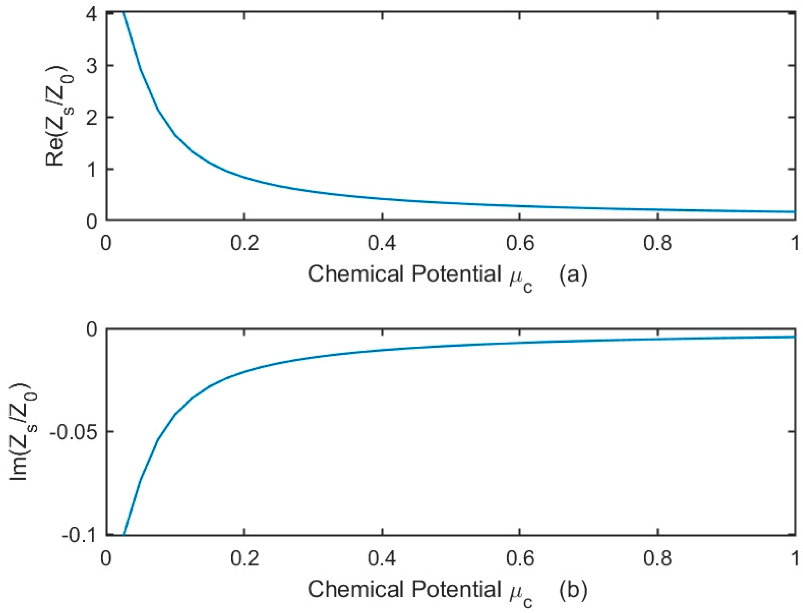
μc > 0.05 eV. The normalized surface impedance using graphene conductivity given in (3) is shown in
Figure 2 in the microwave range.
The graphene conductivity and related surface impedance is almost frequency independent at microwaves and so it exhibits completely different behavior with respect to the THz and optics. Therefore, one can say that even if it is not shown in the plot of
Figure 2, it is almost the same for larger frequencies in microwave range. The other important property is seen in that the surface impedance is dominantly resistive, and the reactive part can be neglected as it is smaller than 2.5% compared to real part. In addition, it can be stated that controlling the chemical potential μ
c with electrostatic biasing, one can control the scattering level and focusing ability of the reflector. Numerically, it can be said that if 0.05 <
μc < 1, then
Zn can change between 4
Zo and 0.1
Zo. This is a practically realizable range where graphene surface varies from very low conductivity (almost invisible) to higher conductivity (approaching good conducting surface).
More specifically, starting from Equations (1) and (2) using auxiliary scalar and vector potentials, the electric field integral equation (EFIE) can be derived in the following form (See [
25] for more details):
where
G is the two-dimensional Green’s function satisfying the radiation condition, i.e.,
, and the angle
is between the normal on
M and the
x-direction. The curve
M can be represented mathematically by the parametric equations given as
, where
. In addition, we define the differential length in the tangential direction along
M as
, where
.
To apply the MAR method to the given problem, we should add and subtract the similar functions from the integral kernels in (4). The subtracted ones with the original kernel produce the following similar functions having smooth behavior without singularity. The latter added ones can be inverted analytically, which helps the derivation of the dual series equations during the procedure of the semi-inversion regularization [
12]:
It can be stated that the functions A and B are continuous, and their first derivatives are also continuous, while their second derivatives with respect to
φ and
φ′ have only logarithmic singularities. This means that second derivatives belong to
. Therefore, on the closed contour
C, their Fourier transforms can be computed numerically by using the efficient Fast Fourier Transform algorithm. Then, all the terms in the SIE (4) with the A and B functions are written in Fourier Series form. By this way, the SIE is discretized and with the zero current condition on the circular part of contour C that is arc S, it constitutes a dual series equation. The details of the derivation of dual series equation are given in [
12]. Then, using the MAR method based on the semi-inversion procedure with the RHP technique [
10,
11], we obtain an algebraic equation. This matrix equation has infinite dimension with the mathematical form of Fredholm second kind, hence the Fredholm theorems guarantee the existence of the unique solution, and also, the convergence of the approximate numerical solutions can be obtained by truncating the matrix with the increasing matrix orders.
The far zone scattered field from the reflector has a mathematical form of cylindrical wave with components
and
, where
is the angular scattering pattern. Then, total scattering cross-section (TSCS) is obtained by using the following equation:
As graphene is dominantly resistive at microwave range, it is a lossy material. In the modelling of the scattering performance of reflector, another important characteristic is absorption cross-section (ACS), which can be found from the optical theorem [
7,
16].
One more parameter that should be studied is the focusing ability (FA), and it can be taken as the total H-field at the geometrical focus of the reflector. The FA is defined mathematically as follows:
where
and its absolute value is unity.
On the other hand, single-layer graphene surface can be realized as the one-layer atomic thickness; therefore, the two-side resistive boundary condition can also be applied to a graphene surface. Then, by applying the resistive BC with the SIE formulation, one can obtain the results for a finite-size parabolic reflector made of graphene using Kubo formula. But if the reflector’s electrical size becomes large, one should choose the smaller ones to simulate in reasonable time. I mean that in the range of 0–100 GHz, our findings work correctly. This was our claim in the paper. Here, by using this procedure, some numerical results are obtained and demonstrated in the following section
3. Numerical Results
In this section, we give the results obtained from the simulation of the problem. These results are produced based on the formulation explained in the previous section, and the figures here show the verification of the method. These results are computed using an available laptop PC with the Intel i7 processor of the 7th generation and 32 GB RAM working on the Windows 10 platform.
From the observation of the plots given in
Figure 2, the normalized surface impedance of the graphene reduces with the increasing chemical potential μ
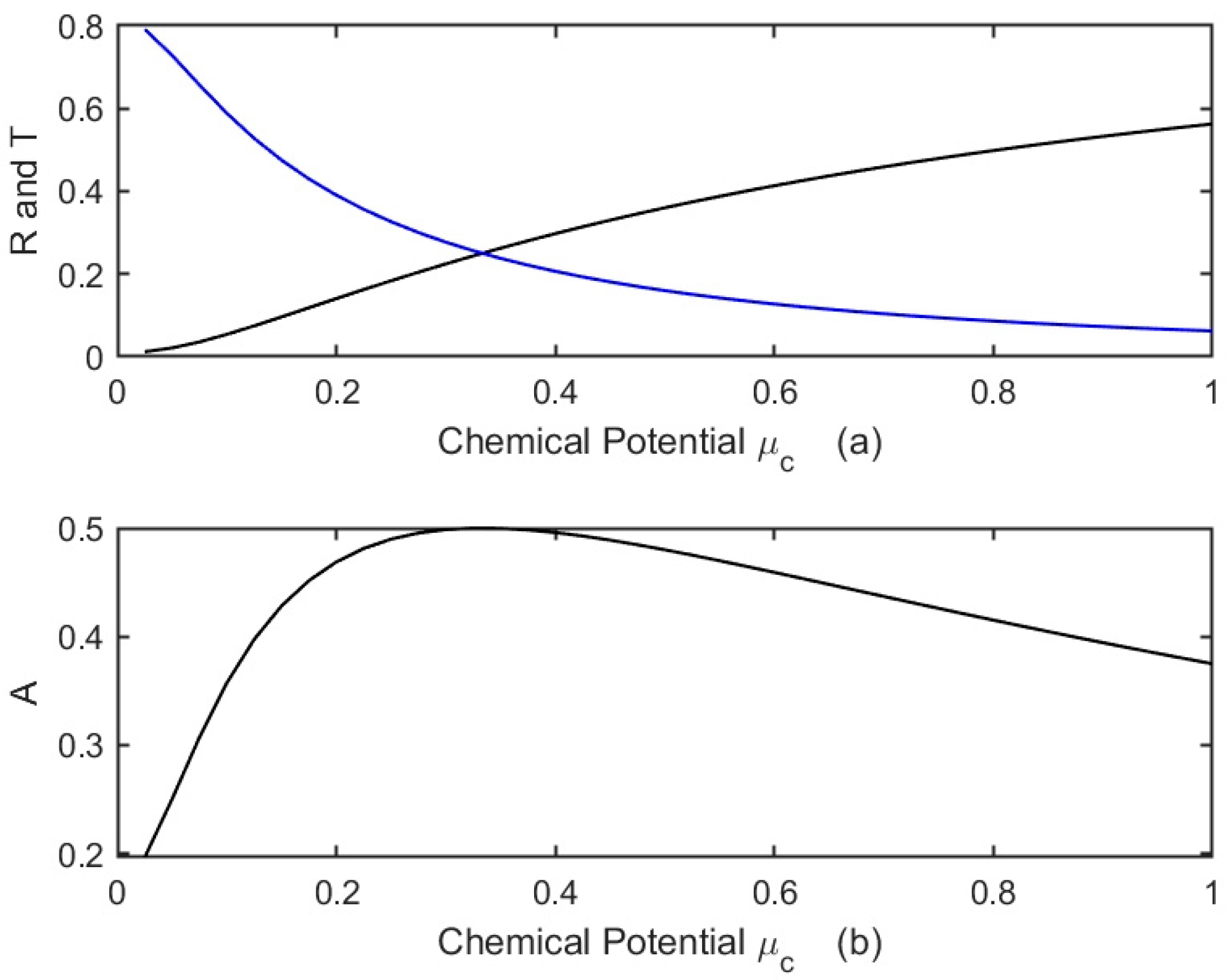
c. Eventually, it approaches the small values of the limit case of the PEC surface. In
Figure 3, the reflectivity (R), transmissivity (T), and absorptivity (A) are demonstrated versus the chemical potential
μc for the plane wave normal incidence to infinite graphene sheet. As expected, the reflected power level increases from small values to the unity with increasing
μc. Therefore, the graphene as a thin resistive layer turns from invisible one to an almost PEC surface. The transmitted and absorbed power levels are also seen to vary according to the power conservation law. Therefore, it can be said that this behavior is almost frequency independent in the microwave range.
Then, we extend our study to a graphene parabolic reflector as a 2D cylindrical structure. Variation of the surface impedance of the graphene with the control of μ
c will change the radar cross section and focusing ability of the reflector. However, before that, we should demonstrate the convergent behavior of the presented MAR method. In
Figure 4, the relative errors in ACS and FA are demonstrated with the increasing truncation number N
tr. A consistent reduction in the relative error is observed, and 4–5-digit accuracy can be achieved in the given range of N
tr.
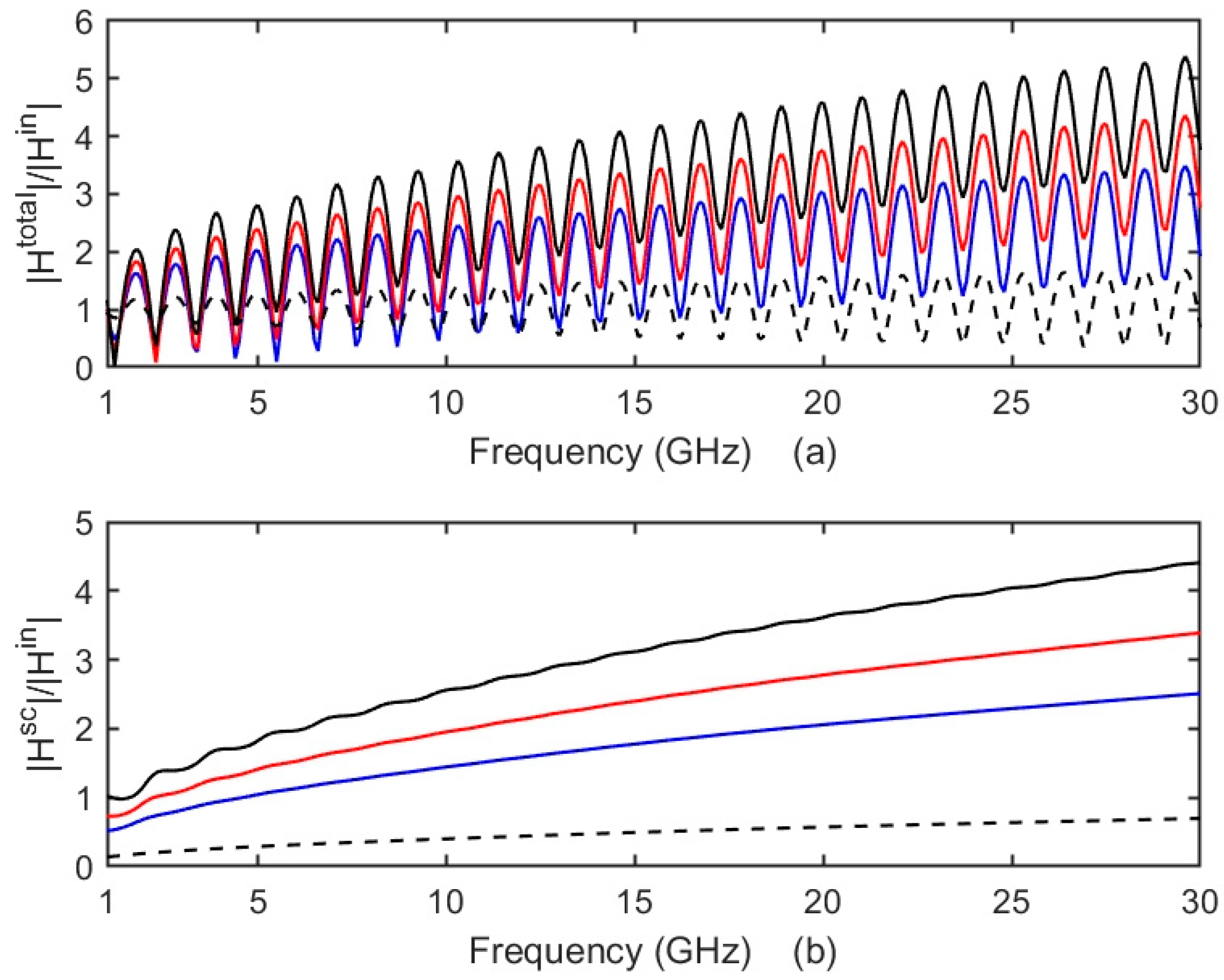
In
Figure 5, the focusing ability parameter is presented in two different ways, as a ratio of the total field to the incident field at the geometrical focus in
Figure 5a and its scattered field counterpart in
Figure 5b. The plots are demonstrated for three different μ
c values. Increasing chemical potential
μc reduces the surface impedance of the graphene reflector and accordingly, the surface reflectivity increases, together with FA. Sharp drop in the graphene’s surface impedance approaches reflector surface to PEC. The presented findings show that 3 times bigger FA can be possible at focus point at most for
μc = 1 eV. In the case of higher chemical potential possibilities, the results will more closely approach PEC, and higher range of control will be possible. This is a limitation of the graphene material. For a very low chemical potential, the surface becomes almost transparent which results in very low surface reflection. These results are also compatible with
Figure 3. As we see in
Figure 5b, the scattered field level varies from 0.8 to 4.3 at 30 GHz, so we can conclude about a controlling mechanism that is possible for the scattered field or FA by adjusting the chemical potential via electrical biasing. The oscillations in part (a) of the figure can be explained by the interference of the scattered field and incident field.
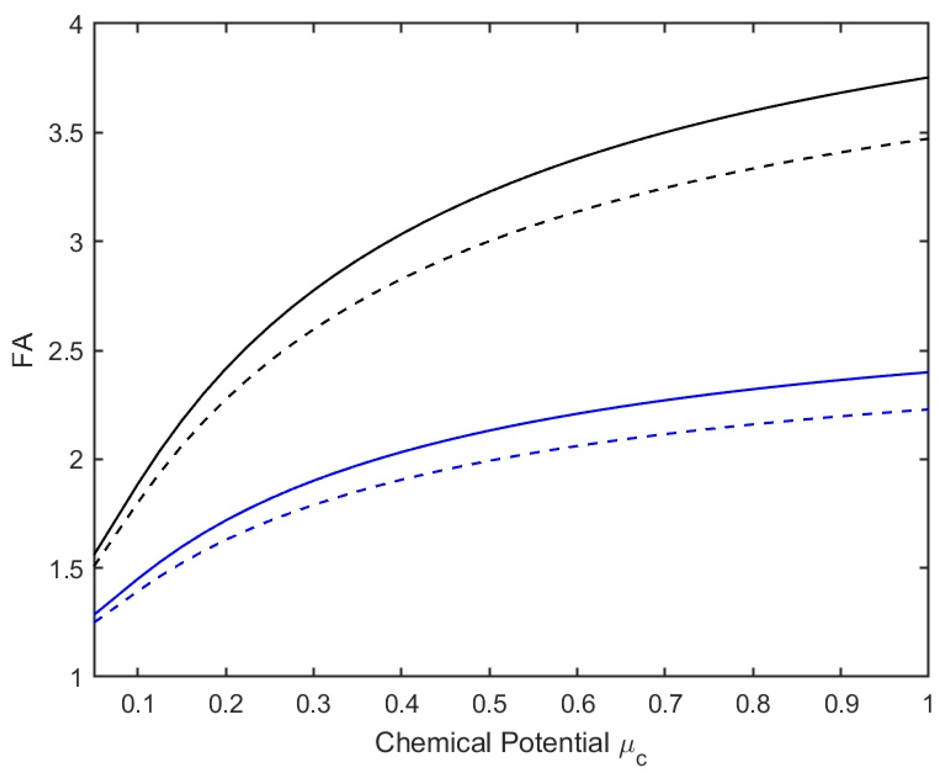
The variation of FA with chemical potential is seen in
Figure 6. As it is visible from the figure, the variation of FA is larger at higher frequency. At 20 GHz, FA varies from 1.5 to 3.7 and closer to PEC case as we see in
Figure 5. It also approaches PEC result at 5 GHz since the size is smaller.
Figure 6 also demonstrates the FA variation for two different f/d values. For a lower
μc value, the reflector is more transparent, so the surface shape has a lesser effect on FA. With the increase of μ
c, the reflectivity of surface increases so the shape of reflector (here, f/d ratio) makes a change in FA plot. It is observed that the deeper reflectors with lower f/d ratio produce smaller focusing field at the focus point. The difference is important for larger μ
c and larger frequencies. This can be realized by considering the surface wave mechanisms on deeper dishes due to the curvature effects.
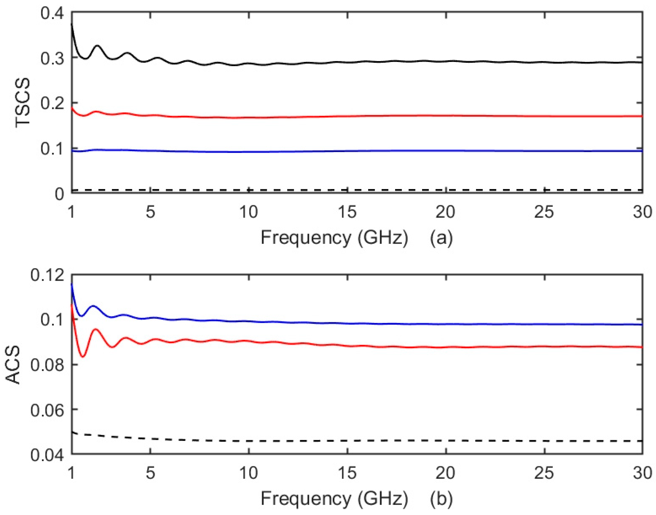
In
Figure 7, TSCS and ACS variation with frequency is presented in the microwave range. Increasing the
μc value increases the graphene surface conductivity, which reduces the surface impedance and so increases the reflector reflection. This can be seen in
Figure 7a for various
μc values. In ACS variation, the maximum variation is observed around the chemical potential value of
μc = 0.4 eV. For chemical potentials higher than that value, ACS reduces, as seen in
Figure 7b, where
μc = 1 eV. This observation is in agreement with
Figure 3b. The oscillations observed in the low GHz range can be explained by the edge effects for the smaller sizes in terms of wavelength.
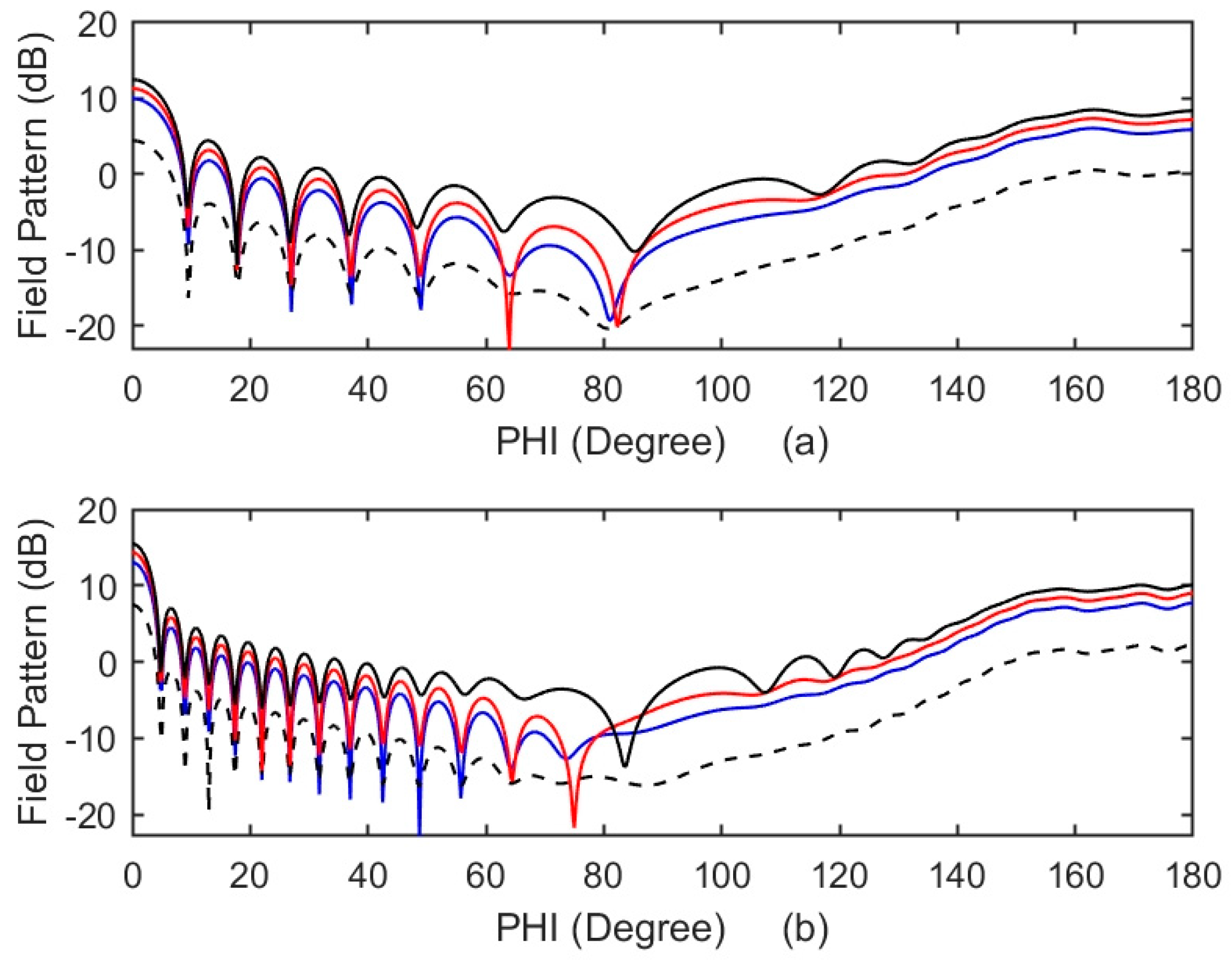
Lowering the chemical potential μ
c reduces the graphene conductivity, so the surface impedance increases, which makes reflector more transparent.
Figure 8 shows that the field reduction is not only seen in the focusing ability but also present in almost all angular directions of the field pattern. For example, around 180°, that is the backward direction, almost 8 dB field reduction can be observed compared to PEC case for
μc = 0.05 eV. If
μc increases towards unity, the scattered field level approaches the PEC surface reflection value, and it is also seen in
Figure 8. This result implies that controlling the reflector by the chemical potential is possible, and it is valid for all directions. This is another important result obtained from the simulation of the presented geometry.
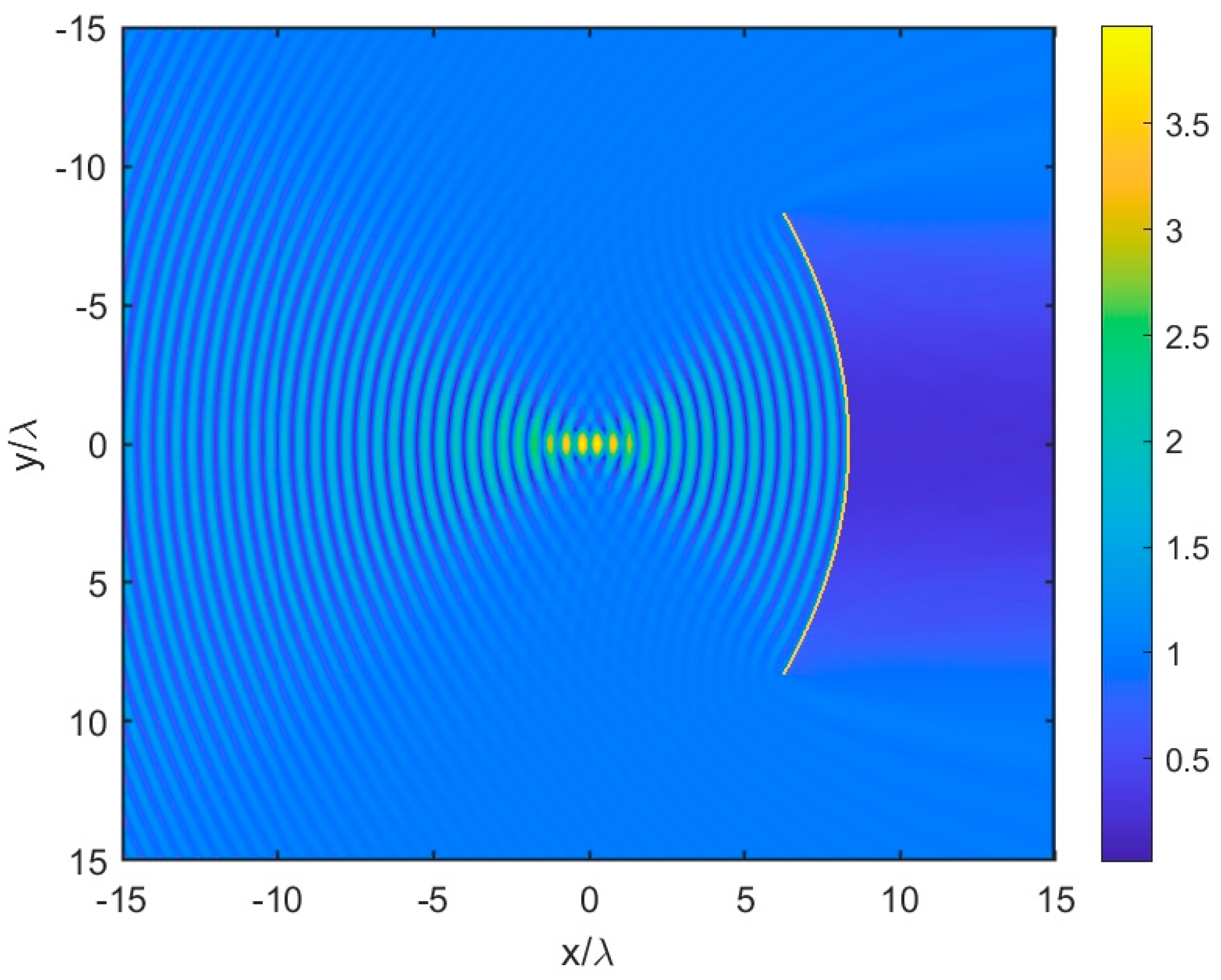
Colored near-field patterns are obtained for the total H-field and shown in
Figure 9 and
Figure 10 for two different chemical potential values. In
Figure 9,
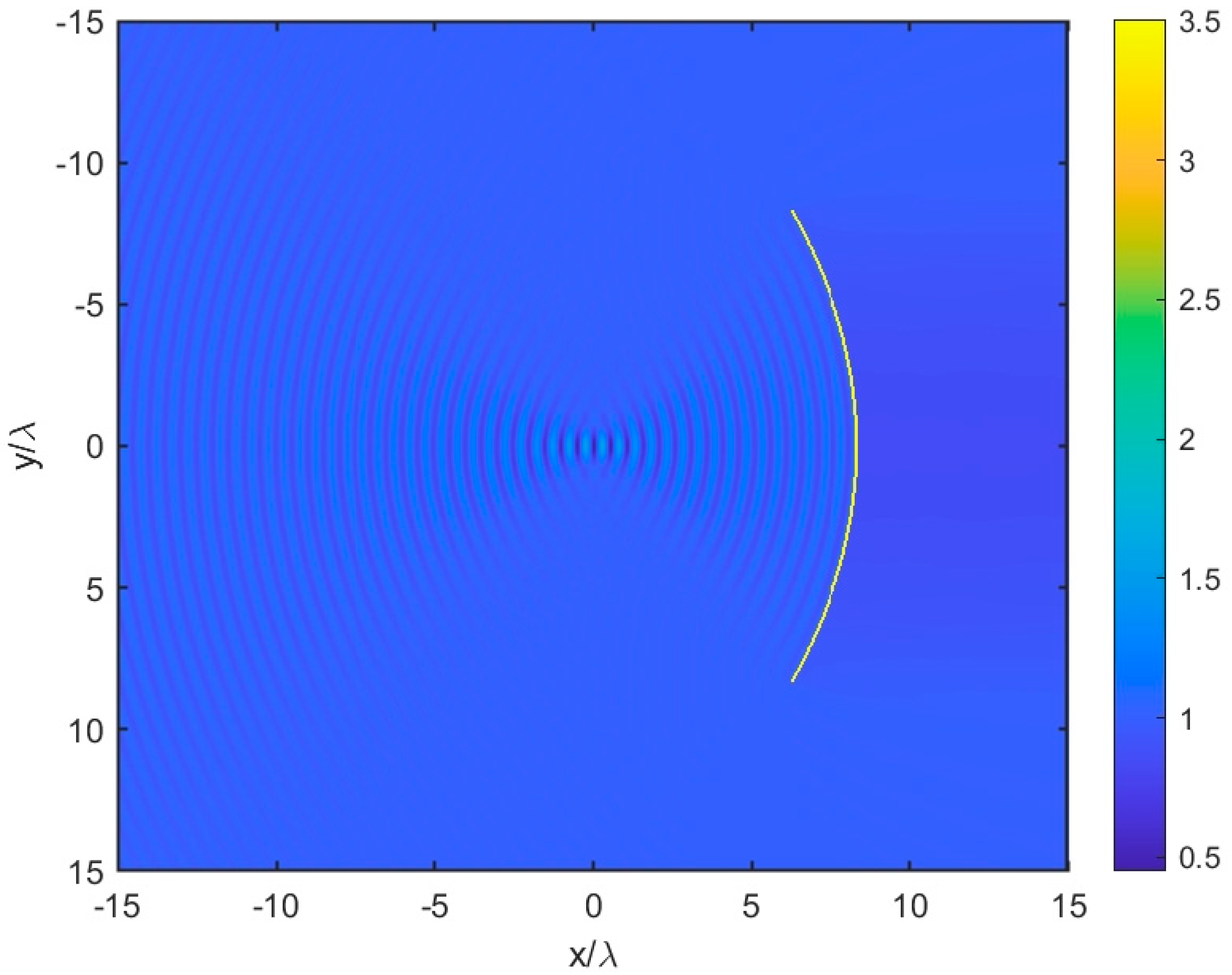
μc is taken as 1 eV, and normalized surface impedance of reflector is smaller compared to the other values of chemical potential. Therefore, the near total field intensity is larger, and it is seen with the yellow color. If
μc is reduced to 0.05 eV as seen in
Figure 10, the total field level sharply reduces especially for the front region of the reflector. It is seen that the reflector loses almost all focusing ability with the reduced chemical potential. Although it is not shown here, the near field takes the intermediate level by adjusting the chemical potential value of the graphene. This result is demonstrated here by using the accurate simulation of the given geometry.

