Abstract
The issue of Electrical Impedance Tomography (EIT) is a well-known inverse problem that presents challenging characteristics. In order to address the difficulties associated with ill-conditioned inverses, regularization methods are typically employed. One commonly used approach is total variation (TV) regularization, which has shown effectiveness in EIT. In order to meet the requirements of real-time tracking, it is essential to acquire fast and reliable algorithms for image reconstruction. Therefore, we present a modified second-order generalized regularization algorithm that enables more-accurate reconstruction of organ boundaries and internal structures, to reduce EIT artifacts, and to overcome the inability of the conventional Tikhonov regularization method in solving the step effect of the medium boundary. The proposed algorithm uses the improved alternating direction method of multipliers (ADMM) to tackle this optimization issue and adopts the second-order generalized total variation (SOGTV) function with strong boundary-preserving features as the regularization generalization function. The experiments are based on simulation data and the physical model of the circular water tank that we developed. The results showed that SOGTV regularization can improve image realism compared with some classic regularization.
1. Introduction
EIT is a non-invasive imaging technology that reconstructs the electrical impedance distribution inside an object by applying a small current to the object’s surface and measuring the resulting voltage response [1]. Since the early 1980s, this technology has gained significant attention in various fields including medicine, industry, and geophysics. Its appeal lies in its non-radiation nature, cost-effectiveness, and real-time monitoring capabilities. In the medical field, EIT finds applications in breast tumor detection, monitoring of brain and abdominal bleeding, and measuring lung function [2].
EIT is a technology that utilizes the surface potential change exhibited by the area being tested [3], along with an appropriate imaging algorithm, to obtain an image of the impedance change in that area. Conductivity distribution changes are associated with pathological changes and physiological activities such as tumors, hemorrhage, ischemia, inflammation, etc. This technology offers several advantages over other methods for monitoring lung injuries [4], including safety, the absence of radiation, real-time monitoring, and visual feedback. It can be effectively used for diagnosing lung diseases and monitoring physiological activities, thereby contributing to the advancement of precision medicine.
The solution to the inverse problem is crucial for achieving the desired imaging effect in EIT technology. It is also a challenging and widely discussed topic in this field. The current difficulties in solving the EIT inverse problem can be summarized as follows: Linear algorithms are known for their fast computation, but they may not accurately reconstruct complex electrical impedance distributions [5]. On the other hand, nonlinear algorithms offer more-accurate reconstructions, although they are computationally expensive and often require good initial guesses [6]. Alternatively, deep-learning-based methods have the potential to provide higher-quality reconstructions and can handle more-complex scenarios [7]. However, these methods demand large amounts of training data and their models are less interpretable.
1.1. Our Contribution
To address the issue of step effects in smooth areas and the loss of edge information during image reconstruction using traditional regularization methods, this paper proposes a SOGTV algorithm for EIT. The proposed method demonstrates superior performance compared with traditional algorithms:
- We propose a SOGTV regularization algorithm that can more effectively smooth the noise of EIT images while preserving the edge information of key lung structures. Compared with traditional algorithms, the new algorithm preserves edges more precisely when processing EIT data.
- To address the dual problem in the SOGTV regularization model, we propose an improved ADMM that combines Nesterov gradient descent and variable orientation multiplier (ADMM) methods. Our algorithm solves the model by leveraging the equivalent form of SOGTV.
- To evaluate the effectiveness of the algorithm, we initially utilized simulation data based on EIDORS for conducting the simulation experiments. Subsequently, we employed the physical model of the circular water tank that we developed to validate our findings. The imaging results clearly demonstrated that our algorithm is capable of accurately identifying the perturbation position of the acrylic cylinder.
1.2. Related Work
During the process of solving the inverse problem of EIT, the amount of measured data is significantly smaller than the amount of data to be solved. As a result, the reconstructed image often has a poor resolution. The traditional Tikhonov regularization method, which is based on the L2-norm [8], leads to blurred reconstructed images because it produces overly smooth solutions. To address this issue, Liu et al. proposed an electrical impedance imaging method that utilizes parameter level sets [9]. Their method greatly improves the resulting image quality by reducing the number of unknown quantities. An effective implementation of the merged total variation and Gauss–Newton algorithm has been accomplished to reconstruct the image in the field of two-dimensional EIT [10]. For this investigation, the process of reconstructing images relied on the utilization of 16 electrodes crafted from copper (Cu) and a neighboring technique for data collection. Song et al. proposed a spatially adaptive TV regularization method [11]. Their method utilizes the difference curvature, an effective spatial feature metric, to identify planar and edge regions. It also employs various image-reconstruction metrics to quantitatively evaluate the obtained reconstruction results, resulting in better robustness and improved resolution for the reconstructed images [12].
In recent years, the development of neural networks has led to the emergence of intelligent algorithms that can selectively train on targeted samples for specific tasks. This approach allows for the utilization of prior knowledge obtained from training, thereby improving the accuracy of model estimation and enhancing the quality of the obtained images [13,14]. In terms of the speed of image reconstruction, although training the model can be time consuming, once the model is trained, the actual image reconstruction process is a one-step imaging technique, which also enhances the imaging speed of the model [15,16]. However, as the demand continues to increase, the cost of training its related models is also rising. This makes it impractical to directly implement these models in clinics and general hospitals.
The EIT electric field distribution is characterized by its soft field nature, resulting in a nonlinear relationship between the boundary measurement voltage and the conductivity distribution in the measured object field. Therefore, the inverse EIT problem is nonlinear [5]. Due to the nonlinearity of the EIT image-reconstruction problem, many solution algorithms, such as the conjugate gradient method [17], attempt to linearly approximate this nonlinear problem. However, this often leads to significant distortion in the resulting image. On the other hand, although the least-squares method utilizes a nonlinear approach to solve the problem, it is still a local optimization method. Consequently, it tends to encounter local minimization problems, resulting in distortion in the reconstructed images [18]. To tackle this problem, the Huber equation is employed to reconstruct the high-order total variation (HOTV) optimization equation [19]. Gong et al. modified the Finite Element Method (FEM) framework for EIT reconstruction by integrating total generalized variation (TGV) regularization. They conducted reconstructions using both simulation and clinical data. The initial findings suggested that, when compared to TV regularization, TGV regularization enhances the generation of more-authentic images [20]. Additionally, auxiliary variables and generalized Lagrange multipliers are introduced to decompose the optimization equation into two simpler subproblems. The fast alternating direction multipliers method is then used to solve the problem. The algorithm demonstrates relatively fast convergence and produces visually improved images while better preserving details, such as edges.
The following is a comparative summary of these regularization methods:
- Traditional TV regularization:Strengths: Good at preserving edges by promoting sparsity in the first derivative of the image. It is well-studied and understood within the community [21].Weaknesses: Can lead to the ‘staircasing’ effect, where smooth transitions are turned into piecewise constant regions. This effect is undesirable in EIT, where smooth conductivity changes are common [22].
- Higher-order TV regularization (HOTV):Strengths: Addresses some limitations of traditional TV, such as staircasing, by considering higher-order derivatives [23].Weaknesses: May not be as effective at preserving fine details as second-order TV, and the selection of regularization parameters becomes more complex [19].Strengths:Specifically designed to overcome staircasing by incorporating second-order derivatives.Balances the preservation of edges and smooth regions better than traditional TV, particularly in EIT, where conductivity distributions can have complex structures [24].Can be more robust to noise and data inconsistencies due to its higher-order nature.
So, we wanted to propose a method designed to overcome staircasing by incorporating second-order derivatives and that balances the preservation of edges and smooth regions better than traditional TV, particularly in EIT, where conductivity distributions can have complex structures.
1.3. Paper Organization
2. Methodology
2.1. The Mathematical Model of EIT
The image-reconstruction problem in EIT involves solving the inverse problem of determining the conductivity distribution inside an object under test by solving for the boundary current and boundary voltage of a low-frequency current field [25]. The EIT system is depicted in Figure 1.
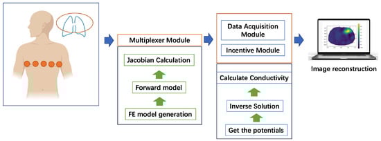
Figure 1.
The framework of EIT image-reconstruction system.
In EIT, the current field is often treated as a quasistatic field, where the potential distribution function and conductivity distribution function within this electric field region satisfy the Laplace equation [26]. The forward operation of the positive EIT imaging problem is used to model boundary voltages:
where is the conductivity vector and F is the forward operator. The reconstruction process is usually stabilized using regularization with the following equation:
where is the forward model prediction of the measured voltage , is the regularization function, is the hyperparameter controlling the level of regularization applied, and is the L2-norm. The function is usually defined in the following form:
The regularization matrix L and the a priori estimate of the conductivity distribution are important components in this context. Various options for the matrix L include unitary matrices, positive diagonal matrices, approximations of the first-order and second-order differential operators, and the inverses of Gaussian matrices. From (2) and (3), we obtain:
The framework represented by this formula is called quadratic regularization because of its use of the L2-norm. The optimization problem for the above framework can be solved by replacing with a linear approximation when making small changes to the initial conductivity distribution .
where J is the Jacobi matrix for the calculation of when the initial conductivity estimate is . Defining and , the following formula is obtained:
This equation is iteratively solved by . The disadvantage is that this technique does not reconstruct step changes, regardless of the choice of L. A smooth solution is preferred.
2.2. TV Regularization
In the field of digital image processing, an image is commonly regarded as a function that requires appropriate modeling. This involves finding the most-suitable function for accurately describing and representing the image. Images often consist of various components such as edges, textures, and noise, each with distinct characteristics. Therefore, it is essential to identify function spaces that effectively capture these different characteristics. Researchers utilize functions within these function spaces to model the various components of an image. The TV regularization method, initially proposed by Rudin, has been widely applied in image denoising [27]. Due to the excellent edge-preserving performance of this method, it has been noticed and improved by a wide range of scholars in the field of image processing.
Fully variational regularization has had a significant impact on image processing and has greatly advanced the use of variational regularization methods in this field. However, it also has limitations. Fully variational minimization tends to provide a minimal solution for the binning constant, which makes it less effective in terms of preserving ‘oscillating’ details such as image textures. Additionally, it is prone to ‘step effects’ in the grayscale gradient regions of the given image. To address the texture-preservation issue, Gilboa introduced the nonlocal total variation (NLTV) regularization method, incorporating the concept of nonlocal methods [28].
In response to the problem that the Tikhonov regularization method smooths edges, resulting in a lower spatial resolution for the reconstructed image, a TV regularization method based on L1 parametrization was introduced [29]. The TV regularization method can enhance the stability of the solution when solving the EIT inverse problem, so as to significantly enhance the resolution of the discrete medium, thus to preserve the discontinuity of the boundary during the reconstruction process and enable the reconstruction of sharp edges to produce sharper images with good edge-preservation performance. Additionally, this method has a better temporal resolution for satisfying the real-time requirements of EIT.
In the measured region , the TV regularization term for the parameter can be defined as:
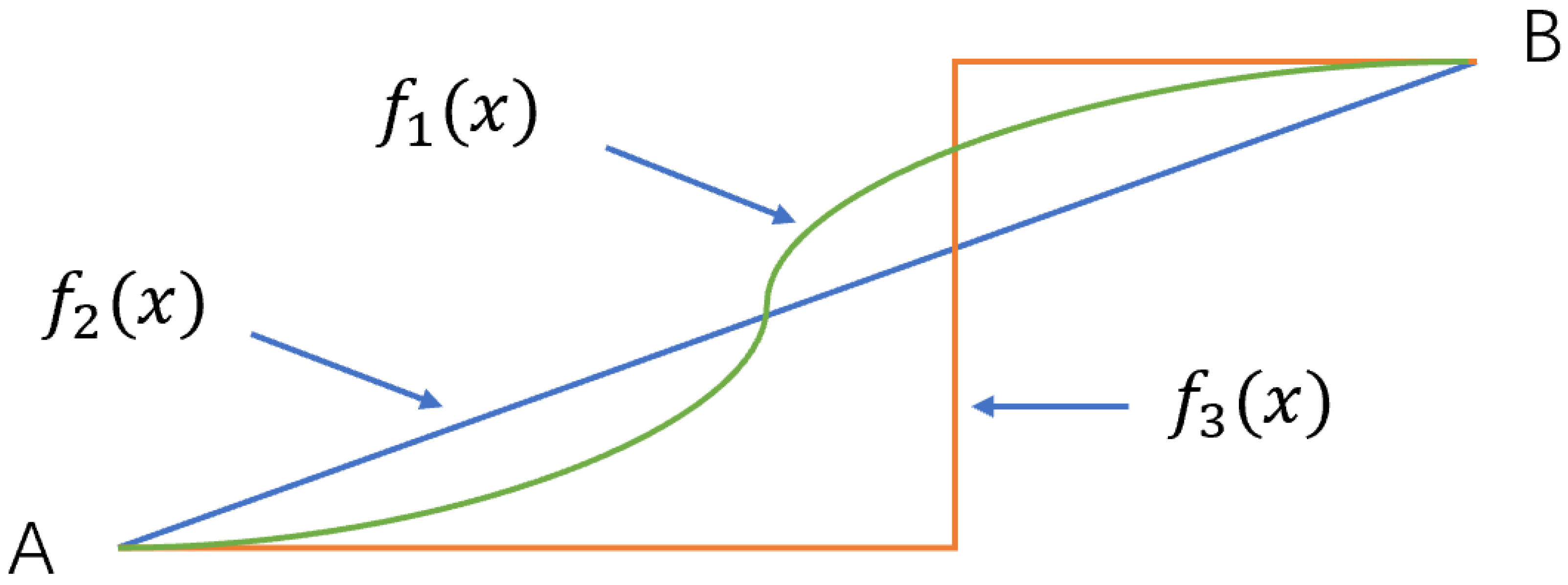
Figure 2 depicts the edge-preserving principle of TV regularization, which can help to understand the edge-preservation properties highlighted by the above equation.
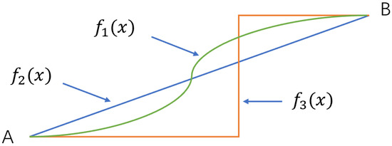
Figure 2.
Three different curves connecting points A and B have the same total variation of the same magnitude.
Points A and B shown in Figure 2 are connected by three curves , , and , and the TVs of the equations of the three curves have the same magnitude, which can be expressed as:
It can be seen that the same TV value allows for different expressions of the function , so when a discrete medium distribution is present in the measurement area, the TV regularization method can effectively reconstruct the edge information and maintain sharp edge characteristics. During EIT reconstruction, the total variance of the change in the conductivity distribution g is used as a TV regularization function:
To derive the above equation:
To prevent the case in which is not differentiable when , a smooth approximation is used to ensure the differentiability of and is expressed as:
where is a positive constant, whose discrete form can be expressed as:
L is the sparse matrix corresponding to the change in conductivity distribution g. The objective function of the TV regularization model can be expressed as:
where A denotes the sensitivity matrix. Equation (13) can be used to solve for the minimal value of the above equation using Newton’s method, where the gradient function can be expressed as follows:
where and diag is a diagonal matrix. The Hessian matrix of Equation (13) can be expressed as:
Therefore, the conductivity distribution can be solved for as follows:
Compared to the Tikhonov regularization method, the TV regularization algorithm effectively captures edge information in discrete media and minimizes the smoothing effect imposed on edges. However, in practical applications, the TV method tends to introduce a ‘step effect’ in smooth areas while resolving sharp edges. This results in a decrease in the overall resolution of the reconstructed image, which limits the applicability of the TV method in EIT. In this study, we propose further improvement and optimization for the TV regularization method to enhance the resolution of reconstructed images.
3. Our Proposed Method
The fully variational regularization problem, which often leads to step effects, can be addressed by incorporating higher-order derivatives [30]. In the literature, several approaches are available for introducing higher-order derivatives. One commonly used method is the TGV proposed by Bredies [31], which combines first-order [32] and higher-order derivative information. TGV effectively preserves image edge details and suppresses step effects, making it successful in applications such as image denoising and MRI [33,34].
Suppose that , and define the following:
where
Equation (17) defines a full variational component for , which is considered as a second-order fully variational component. Additionally, based on Equation (17), the space of second-order bounded variational functions can be defined as follows:
As a further generalization, for , its second-order generalized fully variational component can be defined as follows:
is the weight vector and is a symmetric tensor field with a tight support.
The generalized complete variational fraction of order k can be described more broadly as follows [31]. For a positive integer and , we define a generalized fully variational fraction of order k as follows:
Consequently, the following definition describes the space of generalized complete variational functions of order k.
The definition of provides restrictions with various weights for each , as shown in Equation (21). The weights tend to have a significant influence on the outcomes yielded in practical computations; thus, it must be carefully chosen.
Although the definition in Equation (21) is used for general values of , for two-dimensional images, or is more commonly utilized. In fact, we have that and when :
The following second-order generalized full-variance regularization model is suggested using the second-order generalized full variance concept described above:
where is the observed image with noise; A is the degeneracy operator; and is the image support domain.
The SOGTV, as defined in Equation (14), is challenging to compute. Unlike the first-order generalized TV , which focuses solely on variance [32], the second-order generalized TV also accounts for covariance and constant terms [35]. This necessitates the calculation of additional derivatives and second-order partial derivatives, making its formulation more intricate and computationally demanding. Specifically, involves determining the Hessian matrix of the image function and, subsequently, computing its eigenvalues and eigenvectors. This computational process requires a significant amount of computation and may not be feasible for large-scale problems. Moreover, the regularization term might result in excessively smooth solutions or introduce artifacts in the reconstructed image. However, the second-order generalized full variance can offer more comprehensive information and effectively capture the intricate details and variations in the images and data. As a result, to achieve enhanced computational efficiency, a simplified and easily computable representation of the second-order generalized full variance is commonly employed in practical calculations, as explained in [36].
For the sake of simplicity, we denote , ,
, and . Then,
where , , .
For any closed set B, if its demonstrative function is defined as
, we have
This leads to a relatively concise equivalent expression for , namely
where
Equation (28) reveals that can be understood as a combination of two regularization terms. The first term in Equation (28) demonstrates that approximates and acts as a constraint on the first-order derivative of u. The second term imposes a constraint on the first-order derivative of in all directions, which is equivalent to imposing a constraint on the second-order derivative of u. In the smoothed region, the second term suppresses the step effect, while the first term enables the preservation of edges at the image’s boundaries. The parameters and represent the weights assigned to the two canonical terms in the composite function. However, the selection of these weights in practical problems remains an open question.
The second-order generalized fully variational regularization model can be expressed using the above second-order generalized fully variational equivalence expression, which helps with solving the model. We have proposed an improved alternating direction of multipliers method (ADMM) algorithm for solving the SOGTV problem by combining the accelerated Nesterov [37] and the Fast-ADMM [38].
where is the observed image with noise, A is the degeneracy operator, and is the image support domain.
where and denote the first-order derivative operators along the x and y directions, respectively. Variables and are introduced, and then, the above optimization problem can be equivalently expressed as
Then, the incremental Lagrange function is
The augmented Lagrange function of the given formula is minimized using the improved ADMM. This method yields the following iterative format:
Solve the y subproblem, via the nonlinear contraction operator, as follows,
where .
For the z subproblem, the closed-form solution can be obtained similarly:
where Shrink F.
For the u subproblem, it is necessary to solve its Euler–Lagrange equation as shown below:
To obtain the solution of the p subproblem, the following equation must be solved:
Since both the differential operation and its conjugate operation can be calculated using convolution, the above formula can be computed in the Fourier transform domain by leveraging the fast Fourier transform [39].
Then,
In the formula, F and represent the two-dimensional fast Fourier transform and its inverse transform, respectively. The ∘ symbol denotes the point multiplication operation between matrix elements, and the division operation mentioned here refers to the ‘point division’ operation.
The following Algorithm 1 is obtained for solving the second-order generalized fully variational regularization model.
| Algorithm 1 The algorithm of the second-order generalized regularization model for EIT. |
| Input: |
|
| Output: |
|
4. Experiment
4.1. Metrics
To assess the quality of the EIT image-reconstruction method proposed in this study, we compared the EIT effect of this algorithm with those of four widely used EIT image-reconstruction algorithms. The evaluations of these algorithms are based on three parameters: the peak signal-to-noise ratio (), structural similarity index measure (), and learned perceptual image patch similarity ().
4.1.1. Peak Signal-to-Noise Ratio
The is a metric used to evaluate image quality [40]. It measures the reference value of image quality between the maximum signal and the background noise. When given a grayscale image I and a noise image K of size , the mean-squared error () formula is used.
The is defined as follows:
The units of the are decibels, and a higher value indicates less image distortion. Typically, a PSNR higher than 40 dB suggests that the image quality is nearly identical to the original image. A range of 30–40 dB usually indicates an acceptable image quality distortion loss level. However, a between 20 and 30 dB signifies relatively poor image quality, while a lower than 20 dB indicates significant image distortion.
4.1.2. Structural Similarity Index Measure
The is a metric used to quantify the similarity between two digital images [41]. It is commonly employed to evaluate the quality of a distorted image when compared to an undistorted reference image. Assuming that the original image is x and the reconstructed image is y, the between the two images is evaluated from their brightness, contrast, and structure. The formula for the is as follows:
In the formula, x represents the reconstructed image, while y represents the original image. The brightness is denoted as ; the contrast is ; the structure is .
where and are the mean values of x and y respectively, is the variance of x, is the variance of y, is the covariance of x and y. , , are constant values, and L is a range of pixel values. Let , , and . The values of , , and are all greater than 0. Let , then the simplified SSIM equation is as follows:
4.1.3. Learned Perceptual Image Patch Similarity
The [42], also known as the ‘perceptual loss’, is a metric used to quantify the difference between two images. This metric focuses on learning the inverse mapping between the generated images and ground truths, which helps the generator learn how to reconstruct real images from fake images. It prioritizes the perceptual similarity between the generated and real images, making it more aligned with human perception than traditional methods such as , the , and the . A lower LPIPS value indicates a higher similarity between the two images, while a higher value indicates a greater difference.
The equation is as follows:
where d is the distance between x and . The feature stack is extracted from the L’th layer and unit-normalized in the channel dimension. The vector is used to deflate the number of active channels, and finally, the L2 distance is calculated. Finally, it is averaged over the space and summed over the channels.
4.2. Results
This paper aims to evaluate and compare the effectiveness of the second-order TV algorithm with the existing classic algorithms in terms of their numerical performance. To achieve this, the EIT simulation experiments were conducted using the pyEIT environment in Python 3.10 [43]. The experiment was performed on a Windows 10 64-bit operating system, with an Intel Core i7-10510U CPU 1.80 GHz–2.30 GHz processor and 16 GB of memory. The test data consisted of chest contour point coordinates obtained from EIDORS’s chest simulation, utilizing simulation data from 16 full-electrode adjacent excitation modes [44].
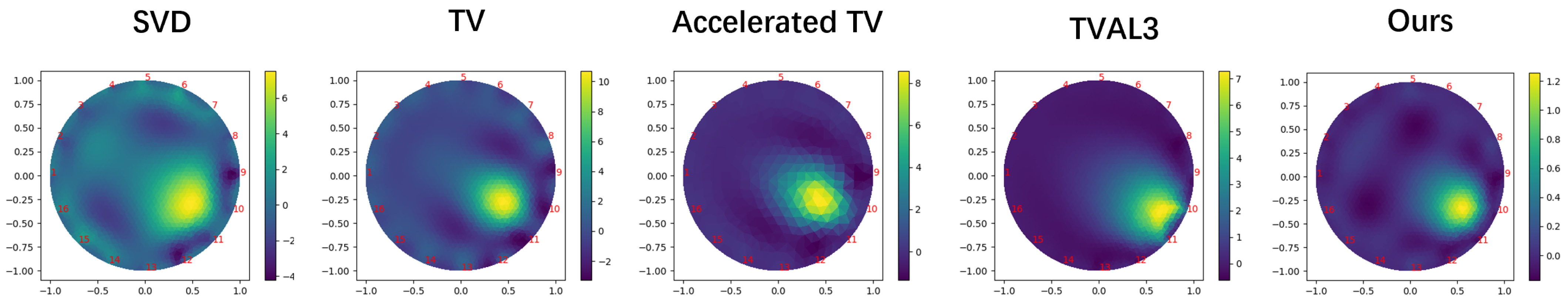
Figure 3 displays the reconstructed images obtained using five regularization methods: Singular-Value Decomposition (SVD) [45], TV [46], Accelerated TV [47], total variation Augmented Lagrangian Alternating Direction Algorithm (TVAL3) [48], and our SOTV method. Upon comparisons, it became evident that the TGV regularization method produced an image with a minimal ladder effect to the naked eye, unlike SVD and TV. The SVD regularization method yielded the lowest image quality, with oversmoothed edges. In comparison to SVD, the TV regularization method significantly improved the reconstructed image quality and better preserved the edge features. The TVAL3 method outperformed the former two methods, particularly in terms of artifact removal. However, all these methods still exhibited a step effect. Nevertheless, the SOTV regularization method effectively reduced the step effect observed in the TV regularization method and avoided the excessive edge smoothing effects in the SVD and TVAL3 regularization methods.
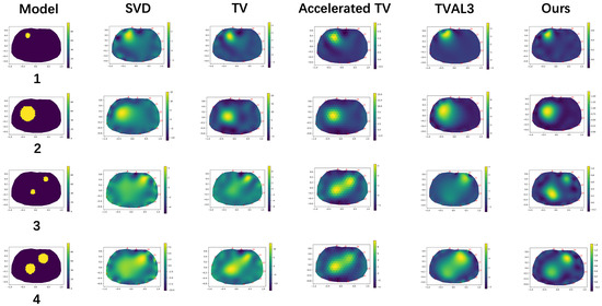
Figure 3.
Reconstruction results produced by the 5 different algorithms.
The analysis described above was based solely on visual judgments and does not establish strong credibility. Therefore, it was necessary to use the two imaging index evaluation methods mentioned in Table 1 to evaluate the specific imaging quality of each method. The two optimal indicators corresponding to the four methods are highlighted in bold black font. The PSNR value of the image reconstructed by the four methods indicated that the SOTV algorithm had the highest PSNR value, demonstrating that it was significantly better than the other three algorithms in terms of suppressing the step effect. Similarly, the calculated LPIPS values also supported this point, as the LPIPS value of the TGV algorithm was the smallest among the four algorithms for the three different models, indicating higher image similarity. However, the LPIPS values of the SVD and TV algorithms were relatively high, suggesting low similarity between the original image and the reconstructed image.

Table 1.
Numerical results reconstructed by different methods for different models.
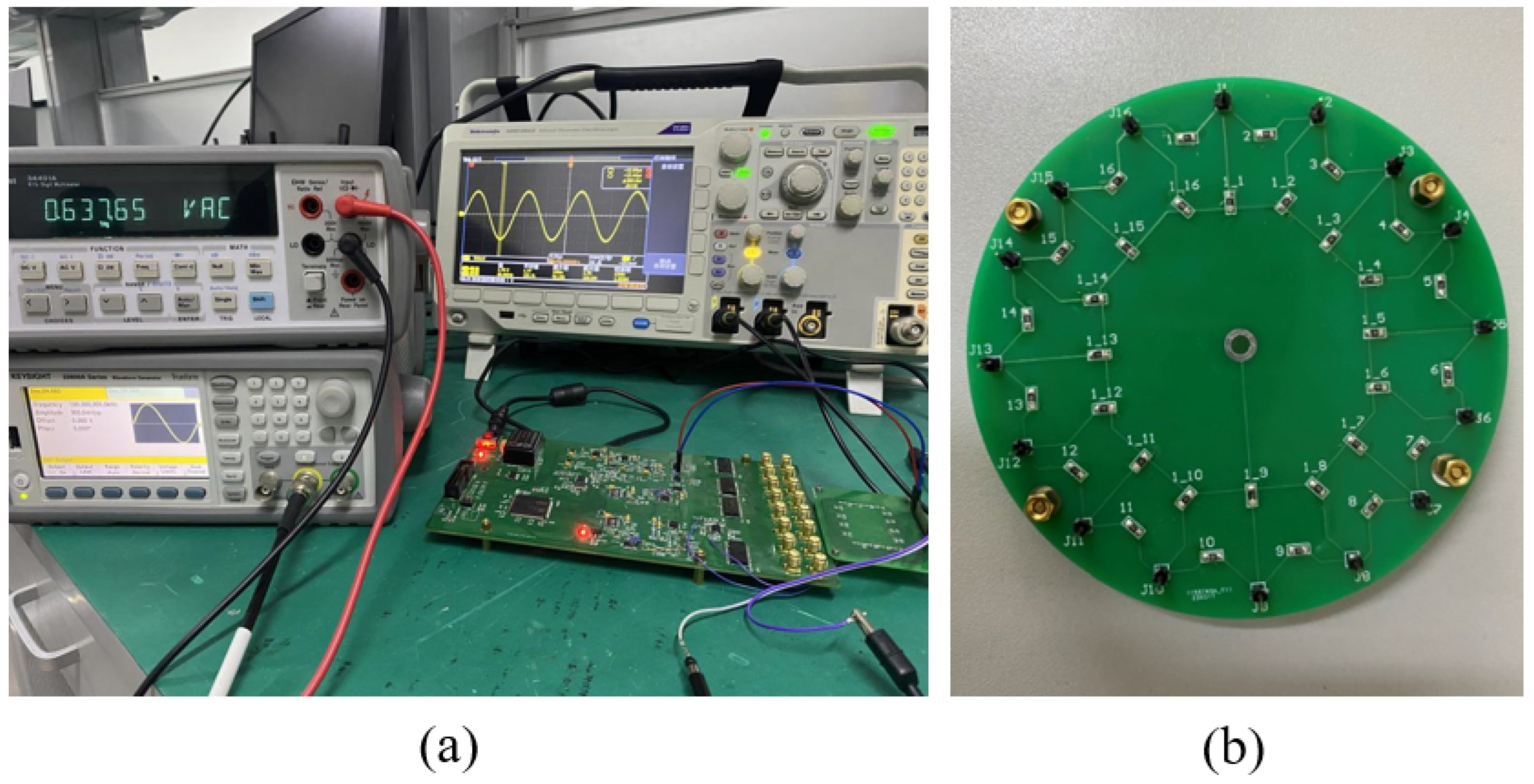
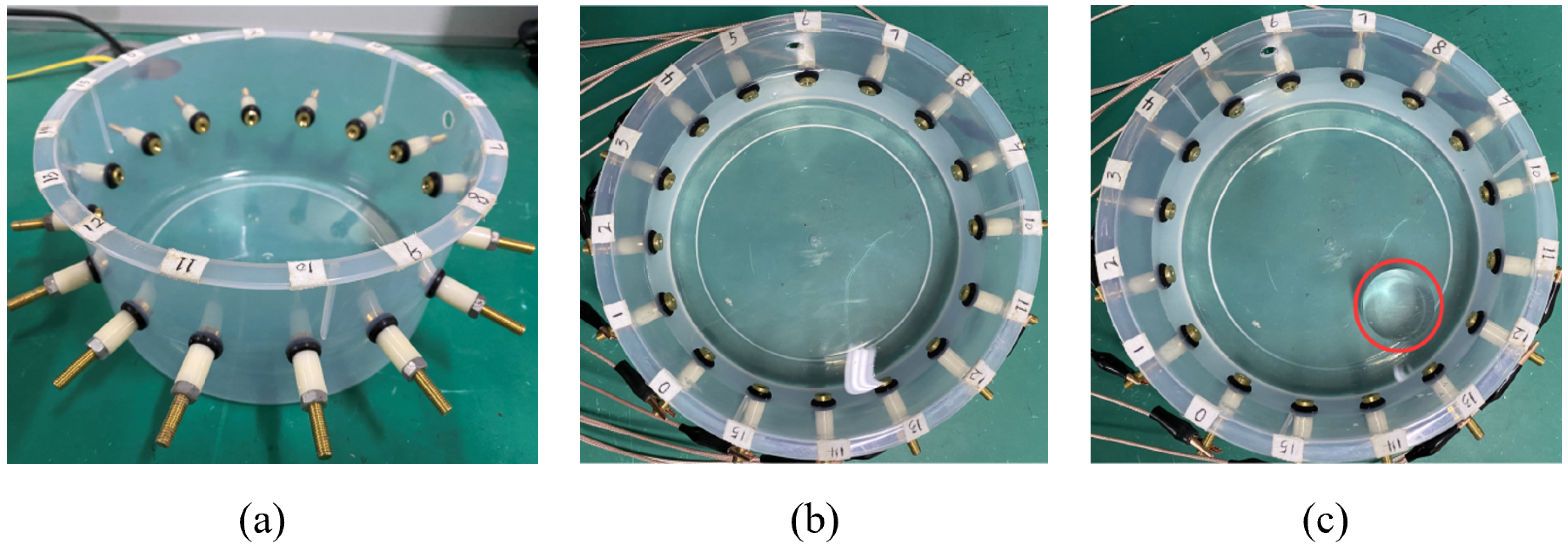
The experiment setup is shown in Figure 4. To replicate the impedance disturbance of the lungs, we constructed a circular water tank physical model in Figure 5a. The model consisted of sixteen electrodes placed at separate holes on the same level of the tank. These electrodes were made of brass pillars with excellent conductivity. To ensure proper sealing and prevent any leakage of experimental liquid that could affect the test results, double-sided silicone rings were used at the holes. The water tank was filled with a solution composed of water and sodium chloride, with a mass ratio of 1000:3 [49], to mimic the environment of biological tissue solution in Figure 5b. Additionally, a 4 cm acrylic cylinder was immersed in the sodium chloride solution within the water tank to simulate the disturbance of intracerebral hemorrhage (Figure 5c).

Figure 4.
An EIT experimental setup. (a) Measured graph of constant current source output current. (b) Resistor loop circuit diagram.
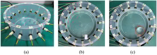
Figure 5.
(a) Physical model of a circular sink. (b) Homogenized sodium chloride solution. (c) With acrylic column.
The experimental process involved fully stirring the prepared sodium chloride solution to ensure an even distribution. The solution was then left to settle for a specific period of time before being transferred into an acrylic cylinder. Once the sodium chloride solution was stable, the excitation current was set to 1 mA, and data were collected at a frequency of 100 kHz. Following the processing and conversion of the acquired data into the pyEIT format, the following Figure 6 was produced.
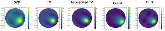
Figure 6.
Visualization of a circular sink with acrylic cylinders using a physical model.
Based on the data provided in Table 2, it is clear that our algorithm surpassed the other methods when considering the evaluation indicators of the SSIM and LPIPS. It secured the second position in terms of the PSNR. Although all three methods produced reconstructed images with artifacts, the ones generated by SOGTV demonstrated the most-effective reduction of these artifacts. It is important to acknowledge that actual measurements may be susceptible to errors in measurement, errors in the model, and interference from environmental noise. As a result, the signal-to-noise ratio of the measured voltage was reduced, leading to a lower quality of the actual reconstructed image compared to the simulated calculation. This further strengthened the conclusion that SOGTV provides superior imaging quality.
Table 2.
Indexes for evaluating tank experiments.
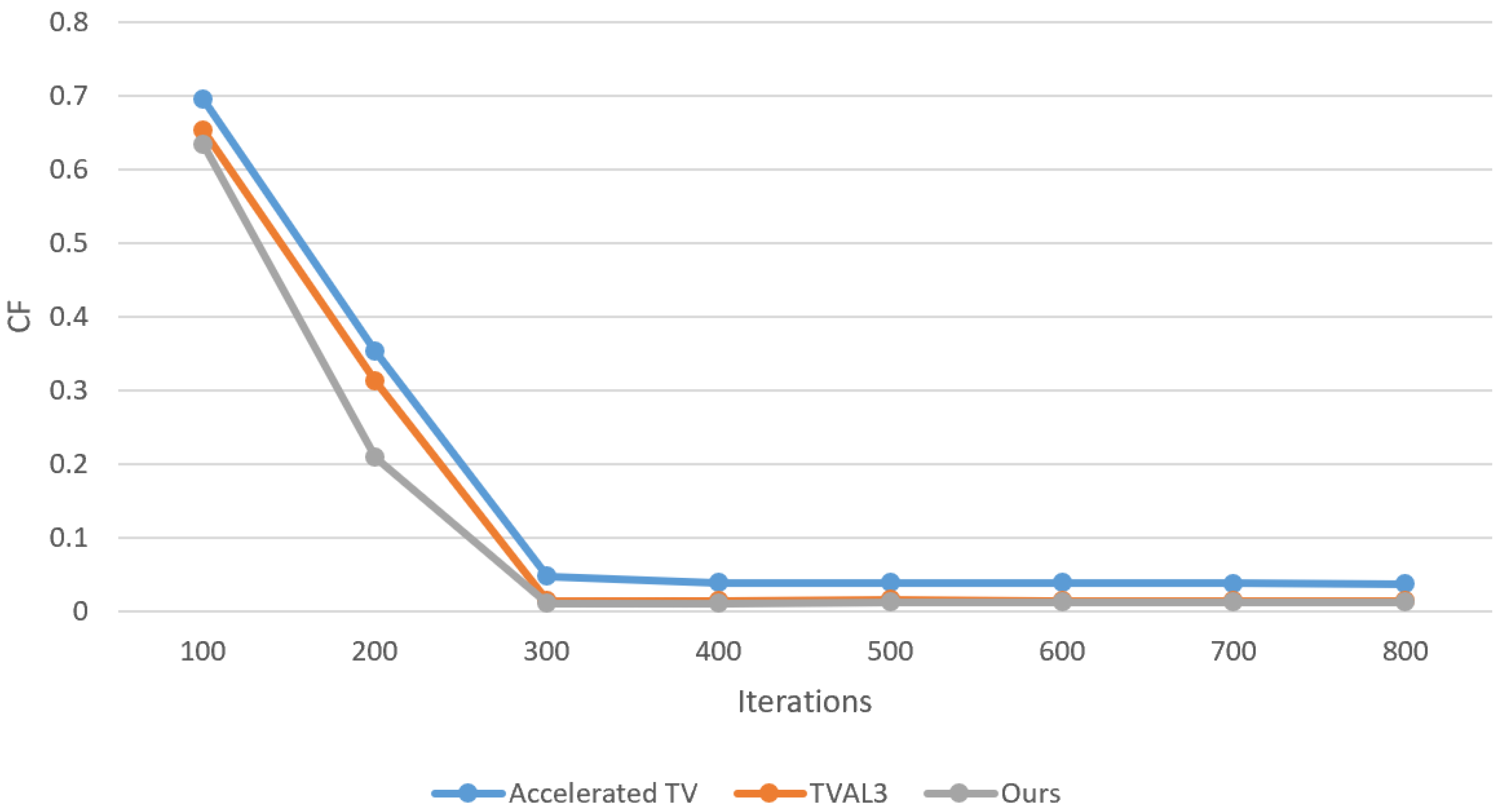
At last, to validate the convergence of the algorithm proposed, numerical experiments were performed. We used the model in Figure 6 and reconstructed the EIT image with three algorithms. As shown in Figure 7, the variation in as the number of iterations progressed is demonstrated. As the number of iterations increased, approached zero. The is calculated as follows [50].
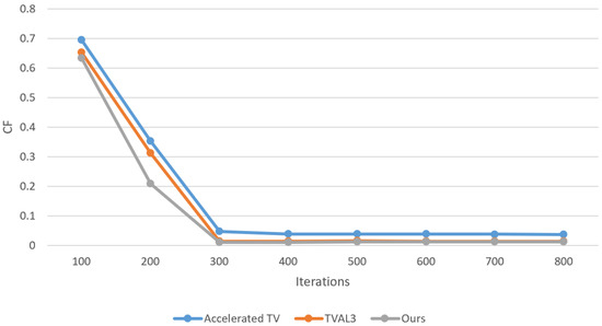
Figure 7.
Convergence rate of the three algorithms (Accelerated TV, TVAL3, SOGTV).
From Figure 7, the SOGTV algorithm has a faster convergence rate compared with Accelerated TV and TVAL3. The imaging results demonstrated that our algorithm effectively identified the perturbation position of the acrylic cylinder. Although some artifacts were still present, a comparison of the relevant indicators confirmed that our imaging quality surpassed that of the other algorithms. This lays a solid foundation for future imaging studies. The research and enhancement of algorithms contribute to new ideas in this field. EIT finds application in various medical imaging fields including lung imaging, breast imaging, and brain monitoring. It serves as a valuable complement to other imaging technologies like X-ray, CT, and MRI due to its advantages in real-time monitoring, non-invasiveness, and cost-effectiveness.
5. Conclusions
This paper proposes a SOGTV algorithm for EIT-based lung imaging. The algorithm was evaluated by comparisons with the SVD, TV, Accelerated TV, and TVAL3 algorithms using experimental simulation models with different sizes and shapes. We developed the physical model of the circular water tank to validate our algorithm. The experimental results demonstrated that the SOGTV algorithm achieved both stable solutions and improved image boundary contrast and sharpness levels compared to those of full-variance-regularized images. The proposed algorithm presents a viable solution for the advancement of electrical impedance imaging in lung research. The effectiveness of our algorithm was verified through simulation experiments and tank experiments. However, the algorithm still has some shortcomings that need to be addressed due to limited experimental conditions. Further optimization is required to improve its performance. Additionally, the algorithm needs improvement in terms of generalization, as it currently struggles to accurately image multi-objective water tank models with complex target conditions. To enhance the generalization ability, it is recommended to increase the dataset or further refine the algorithm.
Author Contributions
Conceptualization, R.Z. and C.X.; methodology, R.Z.; software, R.Z. and W.M.; validation, R.Z.; investigation, Z.Z.; resources, Z.Z. and W.M.; data curation, R.Z.; writing—original draft preparation, R.Z.; writing—review and editing, R.Z.; visualization, R.Z.; supervision, C.X. and W.M.; project administration, C.X.; funding acquisition, R.Z., C.X., Z.Z. and W.M. All authors have read and agreed to the published version of the manuscript.
Funding
The authors thank the anonymous referees, whose constructive comments led to a considerable revision of the original paper. This work is supported by the National Natural Science Foundation of China (61967004, 11901137, 11961011, 72061007, and 62171147) and the Guangxi Key Laboratory of Automatic Detecting Technology and Instruments (YQ20113, YQ20114, and YQ23105).
Institutional Review Board Statement
Not applicable.
Informed Consent Statement
Not applicable.
Data Availability Statement
The data that support the findings of this study will be available from the corresponding author upon reasonable request. The data are not publicly available due to privacy.
Conflicts of Interest
The authors declare no conflicts of interest and the funders had no role in the design of the study.
References
- Adler, A.; Boyle, A. Electrical Impedance Tomography: Tissue Properties to Image Measures. IEEE Trans. Biomed. Eng. 2017, 64, 2494–2504. [Google Scholar]
- Borsic, A.; Halter, R.; Wan, Y.; Hartov, A.; Paulsen, K.D. Electrical impedance tomography reconstruction for three-dimensional imaging of the prostate. Physiol. Meas. 2010, 31, S1–S16. [Google Scholar] [CrossRef]
- Shin, K.; Mueller, J.L. Calderón’s Method with a Spatial Prior for 2-D EIT Imaging of Ventilation and Perfusion. Sensors 2021, 21, 5635. [Google Scholar] [CrossRef] [PubMed]
- Zhang, J.; Patterson, R. Non-invasive determination of absolute lung resistivity in adults using electrical impedance tomography. Physiol. Meas. 2010, 31, S45. [Google Scholar] [CrossRef] [PubMed]
- Colibazzi, F.; Lazzaro, D.; Morigi, S.; Samoré, A. Learning nonlinear electrical impedance tomography. J. Sci. Comput. 2022, 90, 58. [Google Scholar] [CrossRef]
- Zhang, K.; Li, M.; Yang, F.; Xu, S.; Abubakar, A. Electrical impedance tomography with multiplicative regularization. Inverse Probl. Imaging 2019, 13, 1139–1159. [Google Scholar] [CrossRef]
- Adam, E.E.B.; Babikir, E. Survey on medical imaging of electrical impedance tomography (EIT) by variable current pattern methods. J. ISMAC 2021, 3, 82–95. [Google Scholar] [CrossRef]
- Lu, L.; Liu, L.; Hu, C. Analysis of the electrical impedance tomography algorithm based on finite element method and Tikhonov regularization. In Proceedings of the 2014 International Conference on Wavelet Analysis and Pattern Recognition, Lanzhou, China, 13–16 July 2014; pp. 36–42. [Google Scholar] [CrossRef]
- Liu, D.; Smyl, D.; Du, J. A Parametric Level Set-Based Approach to Difference Imaging in Electrical Impedance Tomography. IEEE Trans. Med. Imaging 2019, 38, 145–155. [Google Scholar] [CrossRef]
- Jauhiainen, J.; Kuusela, P.; Seppanen, A.; Valkonen, T. Relaxed Gauss–Newton methods with applications to electrical impedance tomography. SIAM J. Imaging Sci. 2020, 13, 1415–1445. [Google Scholar] [CrossRef]
- Song, X.; Xu, Y.; Dong, F. A spatially adaptive total variation regularization method for electrical resistance tomography. Meas. Sci. Technol. 2015, 26, 125401. [Google Scholar] [CrossRef]
- Varanasi, S.K.; Manchikatla, C.; Polisetty, V.G.; Jampana, P. Sparse optimization for image reconstruction in Electrical Impedance Tomography. IFAC-PapersOnLine 2019, 52, 34–39. [Google Scholar] [CrossRef]
- E, W.; Yu, B. The Deep Ritz method: A deep learning-based numerical algorithm for solving variational problems. Commun. Math. Stat. 2017, 6, 1–12. [Google Scholar] [CrossRef]
- Wei, Z.; Liu, D.; Chen, X. Dominant-Current Deep Learning Scheme for Electrical Impedance Tomography. IEEE Trans. Biomed. Eng. 2019, 66, 2546–2555. [Google Scholar] [CrossRef]
- Khan, T.A.; Ling, S. Review on Electrical Impedance Tomography: Artificial Intelligence Methods and its Applications. Algorithms 2019, 12, 88. [Google Scholar] [CrossRef]
- Capps, M.; Mueller, J.L. Reconstruction of Organ Boundaries With Deep Learning in the D-Bar Method for Electrical Impedance Tomography. IEEE Trans. Biomed. Eng. 2021, 68, 826–833. [Google Scholar] [CrossRef]
- Sun, W.; Zhu, Z.; Zhao, R. A modified LS conjugate gradient algorithm for solving Symm integral equation. J. Guilin Univ. Electron. Technol. 2018, 38, 158–161. [Google Scholar] [CrossRef]
- Theertham, G.T.; Varanasi, S.K.; Jampana, P. Sparsity Constrained Reconstruction for Electrical Impedance Tomography. IFAC-PapersOnLine 2020, 53, 355–360. [Google Scholar] [CrossRef]
- Parisotto, S.; Lellmann, J.; Masnou, S.; Schönlieb, C.B. Higher-Order Total Directional Variation: Imaging Applications. SIAM J. Imaging Sci. 2020, 13, 2063–2104. [Google Scholar] [CrossRef]
- Gong, B.; Schullcke, B.; Krueger-Ziolek, S.; Zhang, F.; Mueller-Lisse, U.; Moeller, K. Higher order total variation regularization for EIT reconstruction. Med. Biol. Eng. Comput. 2018, 56, 1367–1378. [Google Scholar] [CrossRef]
- Pan, Q.X.; Li, Y.; Wang, N.; Zhao, P.F.; Huang, L.; Wang, Z. Variational Mode Decomposition-based Synchronous Multi-Frequency Electrical Impedance Tomography. Inf. Technol. Control. 2022, 51, 446–466. [Google Scholar] [CrossRef]
- Song, X.; Xu, Y.; Dong, F. A hybrid regularization method combining Tikhonov with total variation for electrical resistance tomography. Flow Meas. Instrum. 2015, 46, 268–275. [Google Scholar] [CrossRef]
- Zhou, Z.; dos Santos, G.S.; Dowrick, T.; Avery, J.; Sun, Z.; Xu, H.; Holder, D.S. Comparison of total variation algorithms for electrical impedance tomography. Physiol. Meas. 2015, 36, 1193. [Google Scholar] [CrossRef] [PubMed]
- Li, X.; Wang, W. A high order discontinuous Galerkin method for the recovery of the conductivity in Electrical Impedance Tomography. J. Comput. Appl. Math. 2023, 434, 115344. [Google Scholar] [CrossRef]
- Bikowski, J.; Mueller, J.L. 2D EIT reconstructions using Calderon’s method. Inverse Probl. Imaging 2008, 2, 43–61. [Google Scholar] [CrossRef]
- Borsic, A.; Graham, B.M.; Adler, A.; Lionheart, W.R.B. In Vivo Impedance Imaging with Total Variation Regularization. IEEE Trans. Med. Imaging 2010, 29, 44–54. [Google Scholar] [CrossRef]
- Rudin, L.I.; Osher, S.; Fatemi, E. Nonlinear Total Variation Based Noise Removal Algorithms. Physica D 1992, 60, 259–268. [Google Scholar] [CrossRef]
- Gilboa, G. Nonlinear Eigenproblems in Image Processing and Computer Vision, 1st ed.; Springer Publishing Company, Incorporated: Berlin/Heidelberg, Germany, 2018. [Google Scholar]
- Fan, W. Electrical impedance tomography for human lung reconstruction based on TV regularization algorithm. In Proceedings of the 2012 Third International Conference on Intelligent Control and Information Processing, Dalian, China, 15–17 July 2012; pp. 660–663. [Google Scholar] [CrossRef]
- Burger, M.; Osher, S. Convergence rates of convex variational regularization. Inverse Probl. 2004, 20, 1411. [Google Scholar] [CrossRef]
- Bredies, K.; Kunisch, K.; Pock, T. Total Generalized Variation. SIAM J. Imaging Sci. 2010, 3, 492–526. [Google Scholar] [CrossRef]
- Jung, Y.M.; Yun, S. Impedance Imaging With First-Order TV Regularization. IEEE Trans. Med. Imaging 2015, 34, 193–202. [Google Scholar] [CrossRef]
- Niu, S.; Gao, Y.; Bian, Z.; Huang, J.; Chen, W.; Yu, G.; Liang, Z.; Ma, J. Sparse-view X-ray CT reconstruction via total generalized variation regularization. Phys. Med. Biol. 2014, 59, 2997. [Google Scholar] [CrossRef] [PubMed]
- Knoll, F.; Bredies, K.; Pock, T.; Stollberger, R. Second order total generalized variation (TGV) for MRI. Magn. Reson. Med. 2011, 65, 480–491. [Google Scholar] [CrossRef] [PubMed]
- Brinkmann, E.M.; Burger, M.; Grah, J.S. Unified models for second-order tv-type regularization in imaging: A new perspective based on vector operators. J. Math. Imaging Vis. 2019, 61, 571–601. [Google Scholar] [CrossRef]
- Guo, W.; Qin, J.; Yin, W. A new detail-preserving regularization scheme. SIAM J. Imaging Sci. 2014, 7, 1309–1334. [Google Scholar] [CrossRef]
- Zhang, J.; Peng, Y.; Ouyang, W.; Deng, B. Accelerating ADMM for efficient simulation and optimization. ACM Trans. Graph. (TOG) 2019, 38, 1–21. [Google Scholar] [CrossRef]
- Goldstein, T.; O’Donoghue, B.; Setzer, S.; Baraniuk, R. Fast alternating direction optimization methods. SIAM J. Imaging Sci. 2014, 7, 1588–1623. [Google Scholar] [CrossRef]
- Jun, Z.; Zhihui, W. A class of fractional-order multi-scale variational models and alternating projection algorithm for image denoising. Appl. Math. Model. 2011, 35, 2516–2528. [Google Scholar] [CrossRef]
- Sheikh, H.; Sabir, M.; Bovik, A. A Statistical Evaluation of Recent Full Reference Image Quality Assessment Algorithms. IEEE Trans. Image Process. 2006, 15, 3440–3451. [Google Scholar] [CrossRef]
- Wang, Z.; Bovik, A.; Sheikh, H.; Simoncelli, E. Image quality assessment: From error visibility to structural similarity. IEEE Trans. Image Process. 2004, 13, 600–612. [Google Scholar] [CrossRef]
- Zhang, R.; Isola, P.; Efros, A.A.; Shechtman, E.; Wang, O. The Unreasonable Effectiveness of Deep Features as a Perceptual Metric. In Proceedings of the IEEE Conference on Computer Vision and Pattern Recognition (CVPR), Salt Lake City, UT, USA, 18–23 June 2018. [Google Scholar]
- Liu, B.; Yang, B.; Xu, C.; Xia, J.; Dai, M.; Zhenyu, J.; You, F.; Dong, X.; Shi, X.; Fu, F. pyEIT: A python based framework for Electrical Impedance Tomography. SoftwareX 2018, 7, 304–308. [Google Scholar] [CrossRef]
- Adler, A.; Lionheart, W.R.B. Uses and abuses of EIDORS: An extensible software base for EIT. Physiol. Meas. 2006, 27, S25–S42. [Google Scholar] [CrossRef] [PubMed]
- Clay, M.; Ferree, T. Weighted regularization in electrical impedance tomography with applications to acute cerebral stroke. IEEE Trans. Med. Imaging 2002, 21, 629–637. [Google Scholar] [CrossRef]
- Borsic, A.; Graham, B.M.; Adler, A.; Lionheart, W.R. Total variation regularization in electrical impedance tomography. Inverse Problems 2007, 99–136. [Google Scholar]
- Javaherian, A.; Soleimani, M.; Moeller, K.; Movafeghi, A.; Faghihi, R. An accelerated version of alternating direction method of multipliers for TV minimization in EIT. Appl. Math. Model. 2016, 40, 8985–9000. [Google Scholar] [CrossRef]
- Li, C. An Efficient Algorithm for Total Variation Regularization with Applications to the Single Pixel Camera and Compressive Sensing. Ph.D. Thesis, Rice University, Houston, TX, USA, 2010. [Google Scholar]
- Juan, D.; Suhua, C.; Hong, S.; Shu, Z.; Chaoshi, R. Impact Study and Evaluation of SNR on Different Electrical Impedance Tomography Reconstruction Algorithms. Chin. J. Biomed. Eng. 2012, 31, 807–815. [Google Scholar]
- Zhou, Y.; Li, X. A real-time EIT imaging system based on the split augmented Lagrangian shrinkage algorithm. Measurement 2017, 110, 27–42. [Google Scholar] [CrossRef]


Disclaimer/Publisher’s Note: The statements, opinions and data contained in all publications are solely those of the individual author(s) and contributor(s) and not of MDPI and/or the editor(s). MDPI and/or the editor(s) disclaim responsibility for any injury to people or property resulting from any ideas, methods, instructions or products referred to in the content. |
© 2024 by the authors. Licensee MDPI, Basel, Switzerland. This article is an open access article distributed under the terms and conditions of the Creative Commons Attribution (CC BY) license (https://creativecommons.org/licenses/by/4.0/).