Two-Stage Dimensionality Reduction for Social Media Engagement Classification

Abstract

The high dimensionality of real-life datasets is one of the biggest challenges in the machine learning field. Due to the increased need for computational resources, the higher the dimension of the input data is, the more difficult the learning task will be—a phenomenon commonly referred to as the curse of dimensionality. Laying the paper’s foundation based on this premise, we propose a two-stage dimensionality reduction (TSDR) method for data classification. The first stage extracts high-quality features to a new subset by maximizing the pairwise separation probability, with the aim of avoiding overlap between individuals from different classes that are close to one another, also known as the class masking problem. The second stage takes the previous resulting subset and transforms it into a reduced final space in a way that maximizes the distance between the cluster centers of different classes while also minimizing the dispersion of instances within the same class. Hence, the second stage aims to improve the accuracy of the succeeding classifier by lowering its sensitivity to an imbalanced distribution of instances between different classes. Experiments on benchmark and social media datasets show how promising the proposed method is over some well-established algorithms, especially regarding social media engagement classification.

1. Introduction

Since the majority of real-life datasets hold a large number of dimensions, in the field of machine learning, it is vital to select the most relevant features in order to increase the odds of applications regarding different types of data. In fact, the exponential dependence on the dimension is often referred to as the curse of dimensionality: without any restrictions, an exponential number of observations is needed to obtain optimal generalization [1]. This subject is often related to feature selection, a data preprocessing strategy that has proved to be efficient in preparing data for classification and prediction problems. The most important objectives of feature selection include building simpler and more comprehensible datasets, preparing clean, understandable data, and improving the accuracy of succeeding methods [2].

The recent explosion of data availability has presented important challenges and opportunities for feature selection, increasing the interest in dimensionality reduction methods. Regarding this subject, there are some well-known methods, such as linear discriminant analysis (LDA), whereby a low-dimensional subspace is found by grouping individuals from one class as closely as possible (thereby reducing in-class variance), while separating individuals from different classes as far from one another as possible (thereby increasing between-class variance) [3].

In other words, LDA consists of finding the projection hyperplane that minimizes the interclass variance and maximizes the distance between the projected means of the classes. Similarly to principal component analysis (PCA), these two objectives can be solved by solving an eigenvalue problem with the corresponding eigenvector defining the hyperplane of interest [4].

In fact, PCA provides a complementary perspective on feature transformation. This method, a widely employed technique, focuses on maximizing the total variance of the data by projecting it onto a new set of orthogonal axes, known as principal components. Unlike LDA, which aims to maximize the distance between class means while minimizing interclass variance, PCA seeks to capture the intrinsic structure of the data by retaining the most significant variance across all dimensions.

Similar to LDA, PCA involves solving an eigenvalue problem to determine the principal components and their corresponding eigenvectors. This eigenvalue decomposition results in a set of axes that represent the directions of maximum variance in the original data. While LDA emphasizes the discrimination between classes, PCA provides a comprehensive overview of the overall variability within the dataset [5].

Beyond LDA and PCA, the landscape of dimensionality reduction encompasses a diverse array of techniques, each tailored to specific data characteristics and analytical goals. Singular value decomposition (SVD) is a versatile method that excels in capturing latent semantic structures in large datasets [6], while t-distributed stochastic neighbor embedding (t-SNE) focuses on preserving local relationships [7].

To improve its nonoptimality, LDA-based variations have been developed, which still rely on the homoscedastic Gaussian assumption. Essentially, this refers to the assumption of equal variances—assuming that different samples have the same variance even if they came from different populations [8].

Even though enhancements have been made, sometimes algorithms still do not perform as expected, obtaining subspaces that merge classes that are close, making samples from different classes overlap, and thus leading to unwanted results. This issue is referred to as the class masking problem [9].

Recently, a nonparametric supervised linear dimension reduction algorithm for multiclass heteroscedastic LDA was proposed [10]. The method maximizes the overall separation probabilities of all class pairs. By utilizing this class separability measure, the method places greater emphasis on separating close classes while safeguarding the well-separated classes in the obtained subspace, thereby finding high-quality features and effectively addressing class masking.

The method finds an optimal hyperplane that separates classes with a maximal probability with respect to all possible distributions that exist within the given means and covariance matrices. Grounded on this premise—that based on a target dimensionality, high-quality features can be extracted to a new subset—it is possible to combine this method with LDA roots that aim to maximize the distance between cluster centers of different classes, while also minimizing the dispersion of instances within the same class [11].

By adopting the aforementioned approach as the initial phase of a two-stage process, one can conceptualize a second step aimed at converting the subset of high-quality features into a condensed final space, contingent on the number of cluster centers. This involves addressing a multiobjective optimization problem, leading to a linear transformation that can be implemented on the subset obtained in the first stage.

Inspired by this concept, our paper introduces the two-stage dimensionality reduction (TSDR) approach, a novel method designed for data classification. TSDR not only functions as an independent classifier with its built-in discriminator, but also serves as a standalone dimensionality reduction method for subsequent classifiers.

Validation against benchmark datasets is part of the method’s rigor; however, its primary objective lies in effectively predicting and classifying data from social media datasets. These datasets are affected by the aforementioned challenges, such as the curse of dimensionality, class masking, and imbalanced class distribution. In addition, they are also in the spotlight of a notably ongoing social transformation.

In recent years, there have been remarkable advancements in data technologies, overcoming hardware and software limitations. The storage and analysis of massive datasets are now feasible. Simultaneously, in the era of artificial intelligence (AI), companies are heavily investing in solutions to enhance their understanding of people and their behavior [12].

Social networks, serving as vast repositories of user data, offer insights into preferences, affinities, and various aspects discernible to those who genuinely understand users. This raises concerns about privacy, sparking important debates regarding companies’ efforts to safeguard user information [13].

Major corporations like Meta (Menlo Park, CA, USA,) responsible for platforms such as Facebook and Instagram, are implementing measures to protect and enhance customer privacy. Access to data is consistently restricted, with diminishing allowances for authorized developers. This limitation stems not only from the pressure to uphold user privacy, but also because user information is a valuable asset for these companies [14].

Despite such efforts, public profiles on social networks remain vulnerable to third-party scanning without users’ consent. In many cases, access to APIs or network credentials is unnecessary. Collecting online data from social media and other platforms in the form of unstructured text is known as site scraping, web harvesting, and web data extraction [15]. By exploiting this vulnerability, one can glean various aspects of a specific user via mechanisms that scrape internet pages for raw data.

By processing datasets created through these mechanisms, machine learning methods can be applied to predict patterns and metrics such as post engagement. In other words, it is feasible to predict how many interactions a post from a specific user might gain by considering their follower data. This paper makes a unique contribution by employing the TSDR method to classify social media data and explores the social implications, particularly concerning user privacy.

The remainder of this paper is organized as follows. First, Section 2 outlines important concepts and background information on referenced methods. Section 3 provides the details of our proposed algorithm. Next, Section 4 reports and discusses the results of comparisons between multiple classification methods on standard benchmark classification problems. Finally, Section 5 concludes the paper and discusses potential future research directions.

2. Important Concepts and Background

To assess the relevance of a feature within a given space, we employ the Pearson correlation coefficient ($\rho$). This coefficient, ranging between −1 and 1, quantifies the linear relationship between two variables. For variables A and B, each having N scalar observations, $\rho (A,B)$ is calculated using the formula in Equation (1), where $\mu$ and $\sigma$ represent the mean and standard deviation of each variable [16].

$$\rho (A,B)=\frac{1}{N-1}\sum _{i=1}^N\left(\frac{A_i-{\mu }_A}{{\sigma }_A}\right)\left(\frac{B_i-{\mu }_B}{{\sigma }_B}\right)$$

(1)

In simpler terms, when $\rho$ approaches 1, it signifies a positive linear relationship because both variables increase together. Conversely, when $\rho$ approaches −1, it indicates a negative or inverse correlation: when one variable increases, the other decreases. A $\rho$ close to zero suggests no clear relationship between the two variables.

Another important concept to bear in mind about class separability is the silhouette coefficient (s). This is a metric to calculate the goodness of a clustering technique and its value ranges from $-1$ to 1. For a point i, let $a_i$ represent the average intra-cluster distance (the distance between points within a cluster) and $b_i$ the average inter-cluster distance (the distance between all clusters) [17].

According to Equation (2), we can say that the clusters are spaced well apart from one another when s is close to 1. If the coefficient is around 0, the clusters are indifferent because the distance between cluster centers is not significant. If s is close to $-1$, this ultimately means that the clusters are incorrectly assigned. In short, as the second stage of the proposed method is applied, we expect to notice an increase in the s value.

$$s_i=\frac{b_i-a_i}{\max (a_i,b_i)}$$

(2)

Classification is required in many real-world problems. Although many classification methods have been proposed to date, such as neural networks and decision trees, there are still some limitations associated with these methods. Some lack generalization ability and are sensitive to an imbalanced number of instances in each class. Also, even when some classification methods outperform others in training sets, they may perform worse when applied to new datasets (test sets), an issue known as overfitting.

While not a guarantee of better results, a preprocessed dataset with strongly related features and well-defined cluster centers increases the odds of further applications manipulating these data. Taking into account all the points addressed so far, Section 3 dives deeper into the core of the proposed algorithm, detailing each of the two dimensionality reduction stages.

3. Proposed Algorithm

This section details the proposed method, breaking it down into two stages of dimensionality reduction, hereinafter referred to as TSDR-1 and TSDR-2. Additionally, an optional discriminator for classification is also described. Figure 1 illustrates how the proposed algorithm may be used.

To conduct a comprehensive benchmark of the proposed method, we compare the performance indicators of classification methods applied to the original datasets with those obtained from reduced datasets generated through TSDR. Consider a dataset with N features and L labels. Initially, the dataset undergoes classification using conventional methods. Subsequently, the same dataset undergoes TSDR-1, where it is reduced to d dimensions, which is an adjustable parameter optimized for maximum method accuracy. This reduced subset of d dimensions then undergoes TSDR-2, employing multiobjective optimization to transform it into a final subset of L dimensions, equivalent to the number of classes in the original dataset. The ultimate reduced subset is not only classified using conventional methods, but also with the proposed TSDR discriminator embedded in the process.

3.1. First Stage—Maximizing Separation Probability

The definition of separation probability is mainly based on the minimax probability machine (MPM) [18], which maximizes the probability of the correct classification of future data points. Let x and y denote random vectors in a binary classification problem and suppose that the means and covariance matrices of these two classes are $({\mu }_x,{\Sigma }_x)$ e $({\mu }_x,{\Sigma }_y)$, respectively, with $x,{\mu }_x,y,{\mu }_y,\in {\mathbb{R}}^D({\mu }_x\ne {\mu }_y)$ and ${\Sigma }_x,{\Sigma }_y\in {\mathbb{R}}^{D\times D}$. The MPM maximizes the probability $\alpha$ that two classes lie on two sides of a hyperplane $\mathbb{H}(w,b)=\{z\parallel w^{T}z=b\}$, where $w\in {\mathbb{R}}^D,w\ne 0$, and $b\in \mathbb{R}$. The hyperplane separates the two classes with a maximal probability with respect to all possible distributions with the given means and covariance matrices. This optimal w and the corresponding separation probability $\alpha$ of two classes in the subspace can be derived by solving the following problem [10].

$$\max \kappa \left(w\right)=\frac{\left|w^T({\mu }_x-{\mu }_y)\right|}{\sqrt{w^T{\Sigma }_{x}w}+\sqrt{w^T{\Sigma }_{y}w}}$$

(3)

$$\kappa \left(w\right)=\sqrt{\frac{\alpha \left(w\right)}{1-\alpha \left(w\right)}}$$

(4)

$${\alpha }^{*}\left(w^{*}\right)=\frac{{\kappa }^{*}{\left(w^{*}\right)}^2}{1+{\kappa }^{*}{\left(w^{*}\right)}^2}$$

(5)

In fact, with the class means and covariance matrices of two classes, it is possible to calculate the corresponding separation probability $\alpha$ to quantify the class separability between them in a certain 1-D subspace w. In this way, this probability is used as a class separability measure to drive the dimensionality reduction problem, where the use of the separation probability can effectively solve the class masking problem.

Consider a dataset with C classes, whose conditional distribution of class i is given by $p(x\mid {\mu }_i,{\Sigma }_i)$, where ${\mu }_i$ represents the mean and ${\Sigma }_i$ the covariance. In this way, the probability ${\alpha }_{ij}$ of separation of classes i and j in the subspace w can be calculated as in Equation (6).

$${\alpha }_{ij}\left(w\right)=\frac{{\kappa }_{ij}{\left(w\right)}^2}{1+{\kappa }_{ij}{\left(w\right)}^2}$$

(6)

In this way, substituting Equations (7) and (8) into Equation (6), the probability ${\alpha }_{ij}$ can be described as per Equation (9).

$$k_{ij}\left(w\right)=\frac{\left|w^T({\mu }_i-{\mu }_k)\right|}{\sqrt{w^T{\Sigma }_{i}w}+\sqrt{w^T{\Sigma }_{j}w}}$$

(7)

$${\Sigma }_{ij}=({\mu }_i-{\mu }_j){({\mu }_i-{\mu }_j)}^T$$

(8)

$${\alpha }_{ij}\left(w\right)=\frac{w^T{\Sigma }_{ij}w}{w^T{\Sigma }_{ij}w+{(\sqrt{w^T{\Sigma }_{i}w}+\sqrt{w^T{\Sigma }_{j}w})}^2}$$

(9)

The problem is then solved by finding the optimal 1-D subspace $w\in {\mathbb{R}}^D$, where the sum of the separation probabilities of all pairs of classes is maximized, which can be represented in the form of Equation (10).

$$\max J_{\mathrm{DR}-\mathrm{MSP}}\left(w\right)=\sum _{1\le i\le j\le C}{\alpha }_{ij}\left(w\right)$$

(10)

By observing that ${\alpha }_{ij}\left(w\right)$ is homogeneous with respect to w, we can add the normalization constraint on Equation (10). The optimal subspace $w^{*}$ is given below in Equation (11) and calculated as described in Algorithm 1 once it consists of applying a gradient descent algorithm.

$$w^{*}\in \mathrm{argmax}{J}_{\mathrm{DR}-\mathrm{MSP}}\left(w\right)$$

(11)

Algorithm 1 d—Dimension Reduction via Maximum Separation Probability

Require:  Original dataset $\{X,Y\}={\left\{(x_i,y_u)\right\}}_{i=1}^n$ and target dimension d. Ensure:  Optimal subspace $W^{*}$. 1: Calculate the means ${\mu }_i$ and the covariance ${\Sigma }_i$ for $i=0,1,2,\cdots ,C$. 2: Set $A_0=I$ and $W_0$ as empty. 3: for $r=1$ to d do 4:     Step 1 5:        Update $\upsilon$ following $v^{(t+1)}=v^{\left(t\right)}+{\gamma }^{\left(t\right)}\frac{\partial }{\partial v}{J}_{\mathrm{DR}\text{-}}\mathrm{MSP}\left(v\right)$. 6:     Step 2 7:        $w_r\leftarrow A_{r-1}{v}^{*}$ 8:        $w_r\leftarrow \frac{w_r}{∥w_r∥}$ 9:        $W_r\leftarrow (W_{r-1},w_r)$ 10:     Step 3 11:        If $r<d$ then $A_r\leftarrow (I-w_r{w}_r^T)A_r$ 12: end for

3.2. Second Stage—Multiobjective Optimization

The optimization problem for the second stage is to find a unique transformation function that maximizes the distance between different cluster centers while minimizing the spread between instances within the same class [11]. The cluster center is represented by the arithmetic mean of all the points belonging to the cluster (class). Assume that $X_{m_k\times n}^k$ includes all instances of class k (a subset of $S_k$), where each line corresponds to an instance. We transform each row of this matrix via the function F so that we obtain $Y_{m_k\times p}^k$. We define ${\overrightarrow{a}}^k$, a vector of p dimensions, as the cluster center of all $m_k$ instances in $Y_{m_k\times p}^k$, according to Equation (12).

$${\overrightarrow{a}}^k=\frac{1}{m_k}\sum _{i=1}^{m_k}{\overrightarrow{y}}^i$$

(12)

The vector ${\overrightarrow{y}}^i$ is the i-th row of $Y_{m_k\times p}^k$. We also define the scalar $v^k$ as the norm of the eigenvalues of the covariance matrix of $Y_{m_k\times p}^k$, according to Equation (13).

$$v^k=∥\mathrm{Eig}\left(\mathrm{Cov}\right(Y_{m_k\times p}^k\left)\right)∥$$

(13)

We determine Cov(.) to be the covariance operator and Eig(.) to be the calculation of the eigenvalues of the input matrix. The value of $v^k$ indicates how many instances of class k are distributed around its center through its most important directions (eigenvectors). The objective of the method is to adapt the F transform so that $v^k$ is minimized for all k, while the distances between the cluster centers are maximized. This can be formulated as a multi-objective optimization problem, as per Equation (14), and calculated as described in Algorithm 2.

$$\Omega =\left\{\begin{array}{cc}\max ∥{\overrightarrow{a}}^i-{\overrightarrow{a}}^j∥\hfill & \mathrm{for}\mathrm{all}j>i\hfill \\ \min v^i\hfill & \mathrm{for}\mathrm{all}i\hfill \end{array}\right.i,j\in \{1,\cdots ,c\}$$

(14)

In this work, Equation (14) is solved by finding the minimum of the unconstrained multivariable function $\Omega$ using a derivative-free interior-point method [19]. In other words, a nonlinear programming solver is used to search for the minimum of the function and thus to find the optimal coefficients.

From the matrix, once the coefficients have been found, a matrix product is produced between it and the high-quality features subset obtained in the first stage. This results in the final (and reduced) subset are to be forwarded to subsequent methods. As in linear discriminant analysis, the proposed algorithm can be used only as dimensionality reduction method for a subsequent classifier or also as a classifier itself when using the proposed built-in discriminator described in Section 3.3.

Algorithm 2  Multiobjective Optimization

Require:  Subspace $W^{*}$ (hereby referred as x) from the first stage. Ensure:  Optimal subspace $\{X,T\}$. 1: Step 1 2:    Solve $\Omega$ following $\Omega =\min \frac{\gamma +{\sum }_{k=1}^c{v}^k}{{\left({\prod }_i^c{\prod }_{j=i+1}^c∥{\overrightarrow{a}}^i-{\overrightarrow{a}}^j∥\right)}^{\frac{1}{c(c-1)}}}$. 3: Step 2 4:    Find the subspace X by calculating $X=\Omega \times x$. 5: Step 3 Optional discriminator 6:    Step 3.1 7:       Find the distances between the individuals of the new subspace X 8:       to their respective cluster centers by calculating Equation (15). 9:    Step 3.2 10:       Find the classification vector T by considering the smallest index found 11:       for each individual.

3.3. Discriminant Function for Classification

Considering the final subset, a discriminant function can be used to determine which class an individual belongs to, evaluating its distance from the cluster centers of all available classes. In this way, the smaller the value is, the greater the probability that the instance belongs to a specific class is, as per Equation (15).

$$f_k\left(\overrightarrow{y}\right)=\frac{D_k}{{\sum }_{j=1}^c{D}_j}$$

(15)

The discriminant function, defined by $f_k\left(\overrightarrow{y}\right)$, where $D_k=∥\overrightarrow{y}-{\overrightarrow{a}}^k∥$, can be interpreted as the probability of $\overrightarrow{y}\in S_k$, since $f_k\left(\overrightarrow{y}\right)\in [0,1]$. In other words, the smaller the value of $f_k\left(\overrightarrow{y}\right)$, the greater the probability of an individual y belonging to class k. From this point on, the results are converted from generative to actual classification results.

3.4. Data Visualization Experiments

One way to assess the proposed method’s effectiveness is by visualizing its effects on a given dataset. Consider the crab gender (CG) dataset, incorporated into sample datasets from MATLAB R2020a. In CG, there are 200 individuals equally distributed between 2 classes and characterized by 6 different attributes [20].

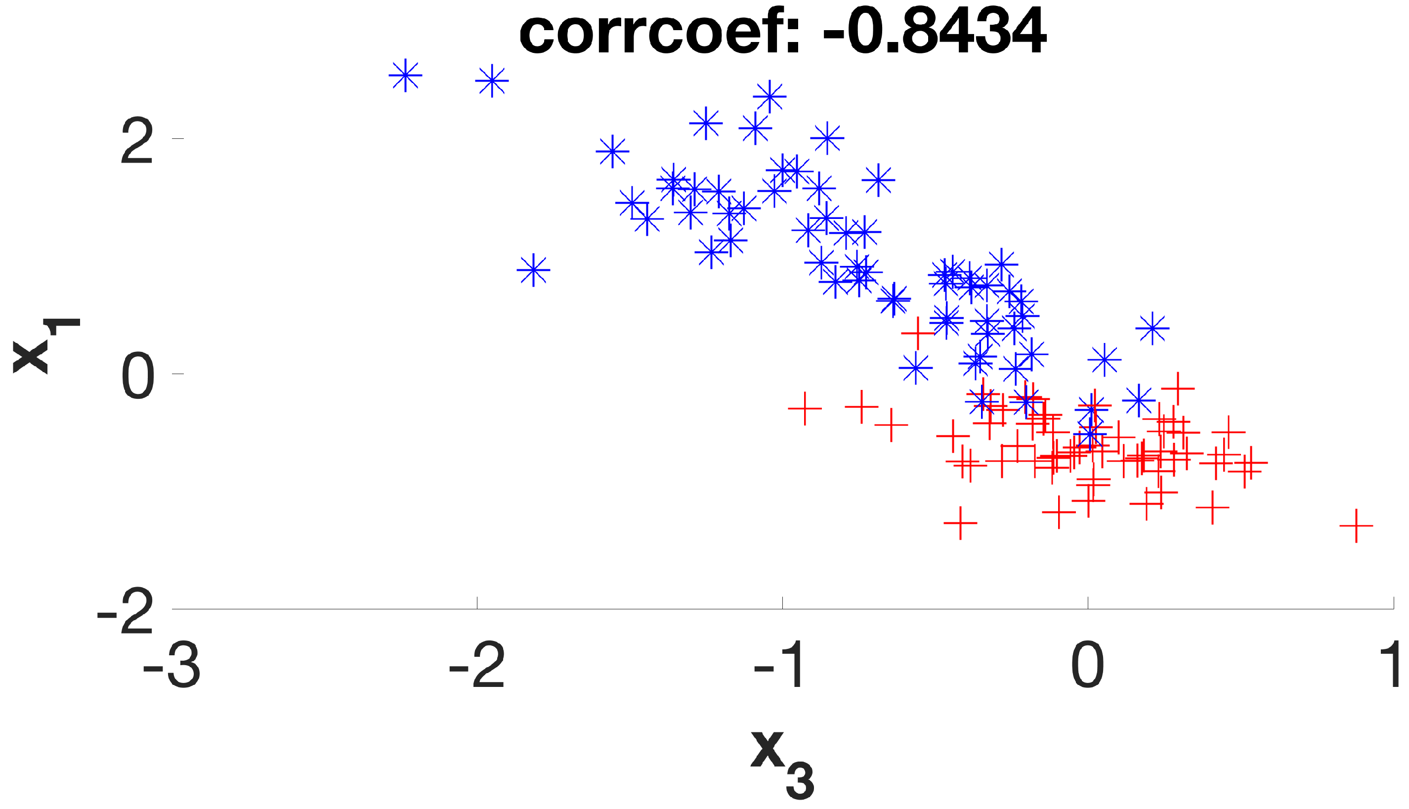
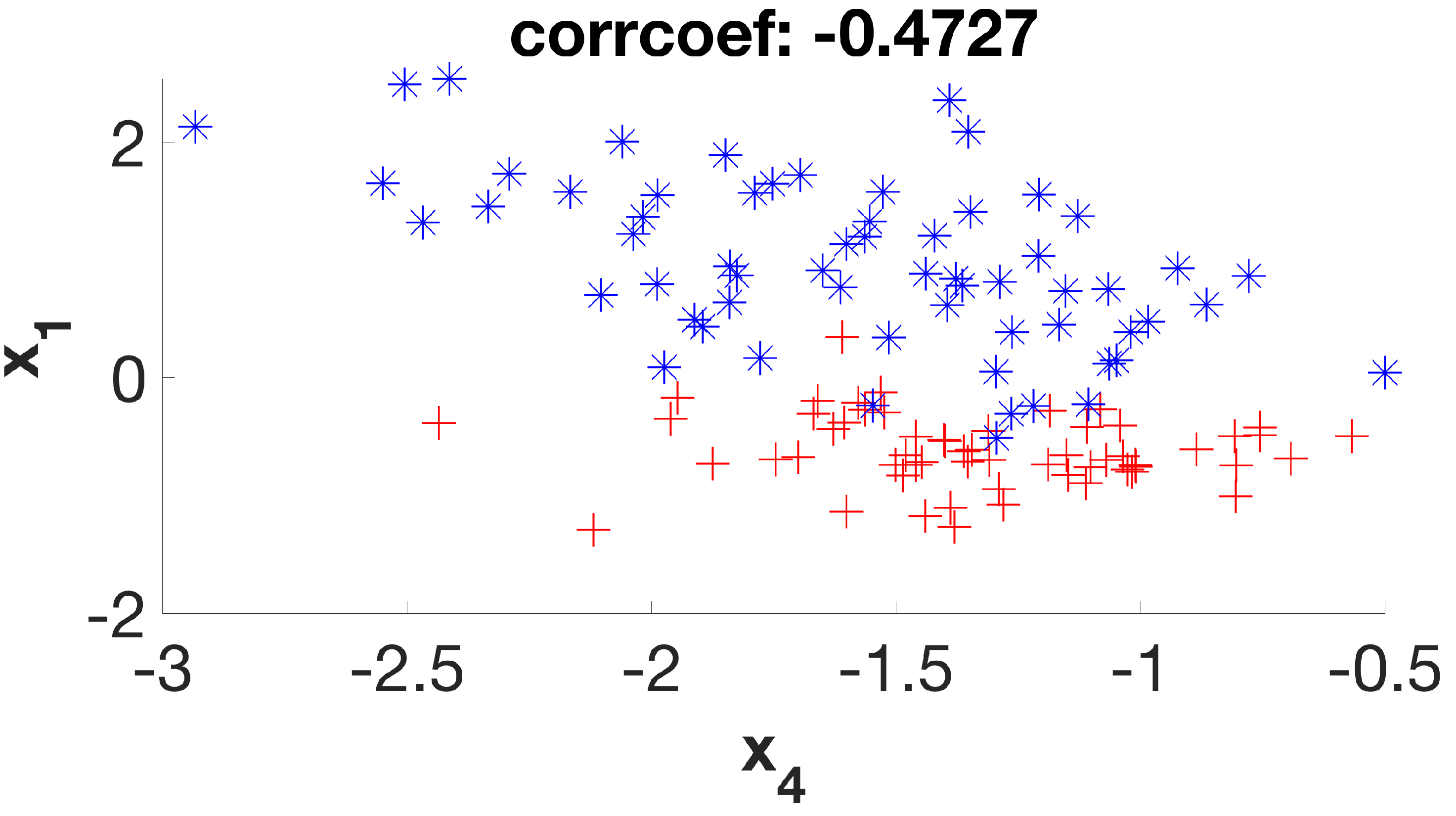
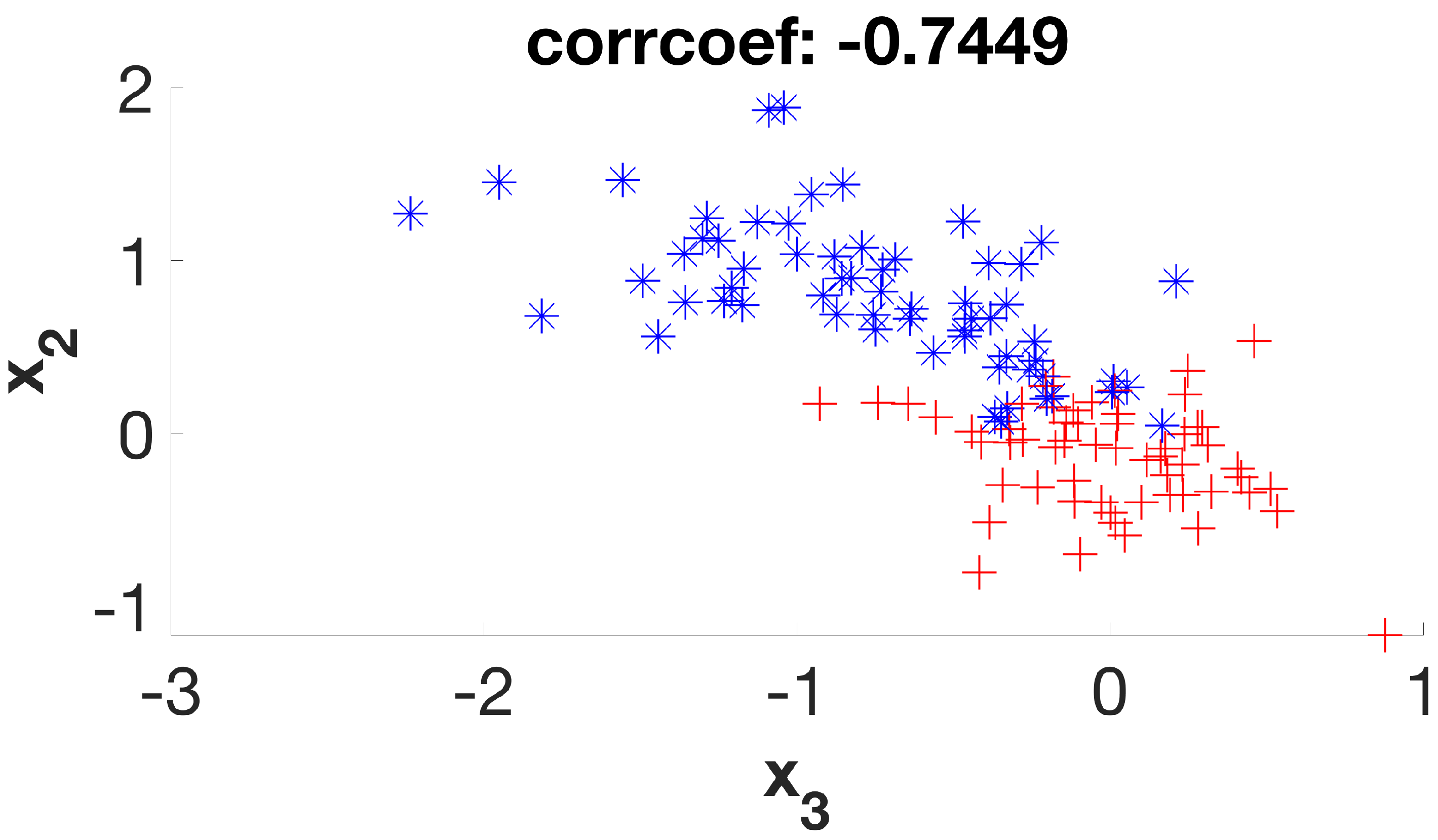
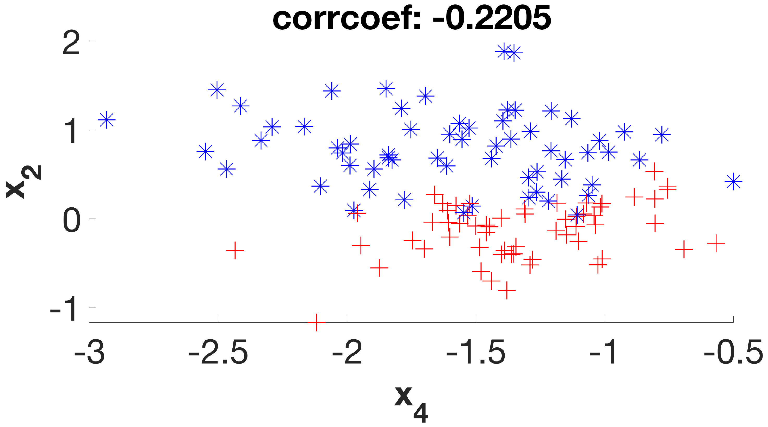
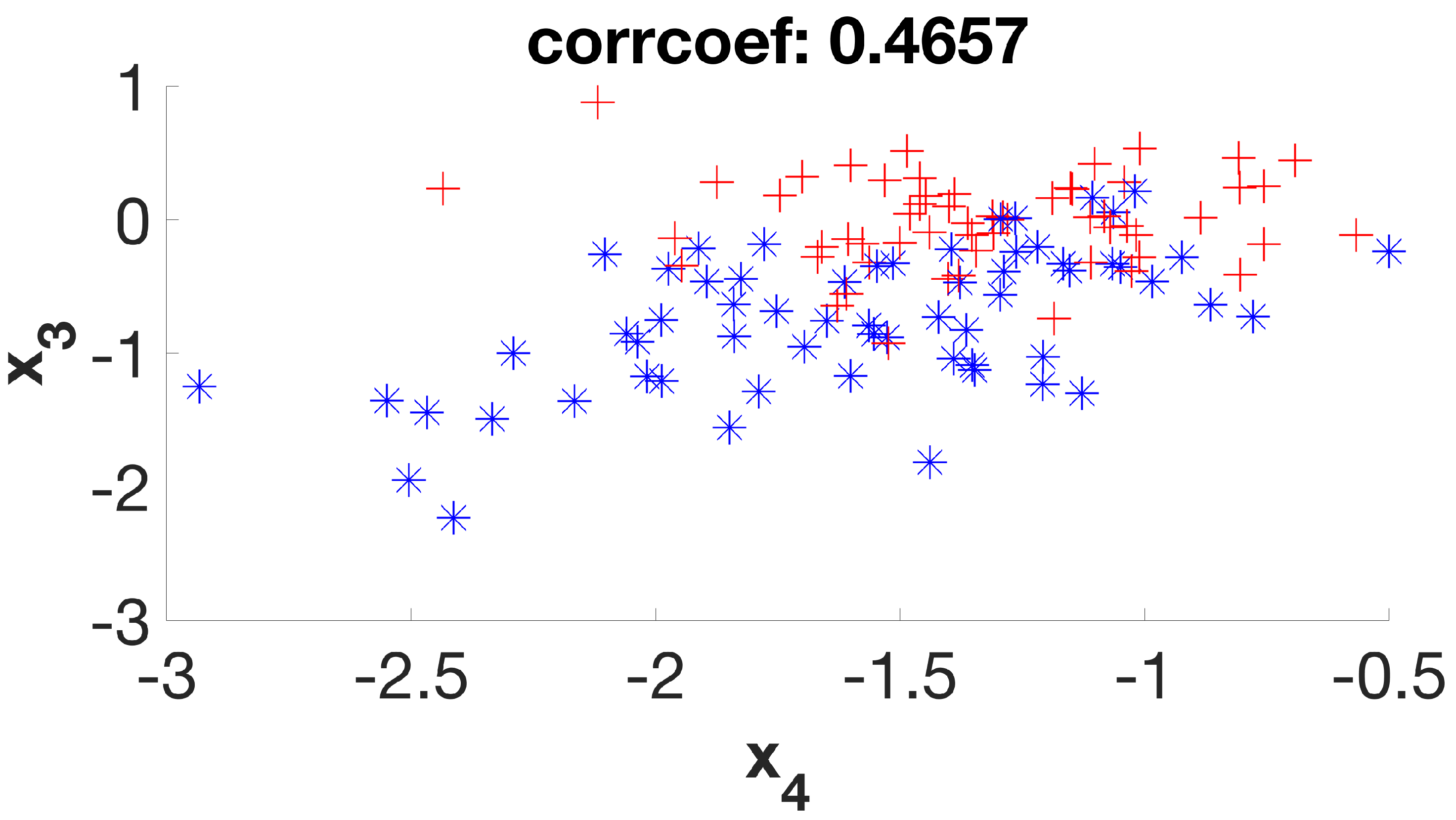
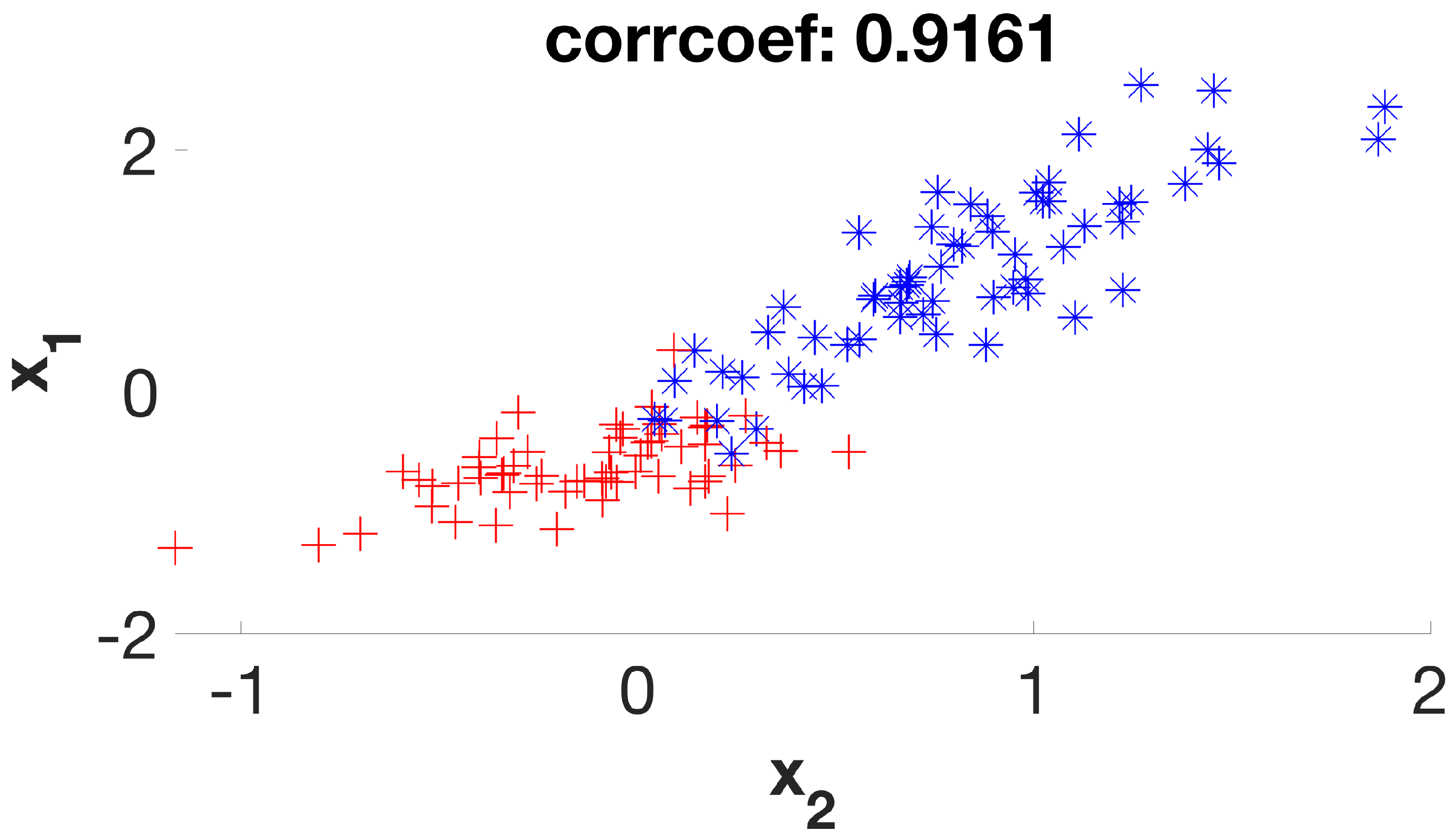
It is a simple dataset that allows us to graphically evaluate the distribution of individuals according to their respective classes. Considering its six initial features (or dimensions), the first stage of the method will create a new subset of four new features (D1 to D4) that will be used in the second stage, which will be expected to deliver a final subset with two remaining dimensions. By examining the scatter plots (Figure 2, Figure 3, Figure 4, Figure 5, Figure 6 and Figure 7) of the six possible variable correlations at the end of the first stage, it is possible to visually assess how the method addresses the class masking problem by separating individuals of different classes.

It is possible to verify that the points on the graphs are much more separable, with few overlaps between them, as the algorithm steps are applied to the dataset. In this way, the following classification algorithm will receive a dataset that—theoretically—has a higher degree of distinction between its individuals when compared to the original set, increasing its chances of presenting greater accuracy.

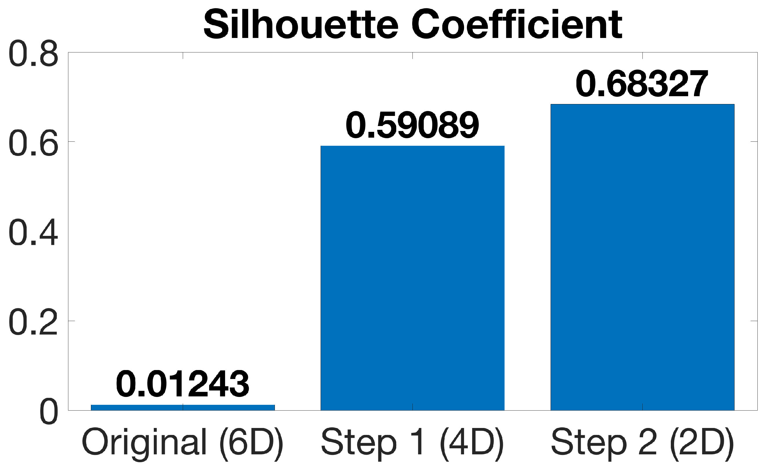
Nevertheless, since accuracy is a subject set to be discussed in Section 4, it is possible to analyze how the silhouette coefficient and the Pearson correlation coefficient change throughout each stage for the crab gender dataset by examining Figure 8 and Figure 9 as per Section 2. Note that Figure 9 shows the average Pearson correlation coefficient by considering the relation between all variables for the crab gender dataset in the original, stage 1, and stage 2 representations.

The silhouette coefficient is roughly 45 times higher by the end of the first stage and 90 times higher in the final subset when compared to the original dataset, increasing as the methods are applied. On the other hand, the average Pearson correlation coefficient [21] is lower at the end of the first stage, but then increases higher than the original value at the end of the second stage. In other words, classes are more easily distinguishable when meaningful features are preserved.

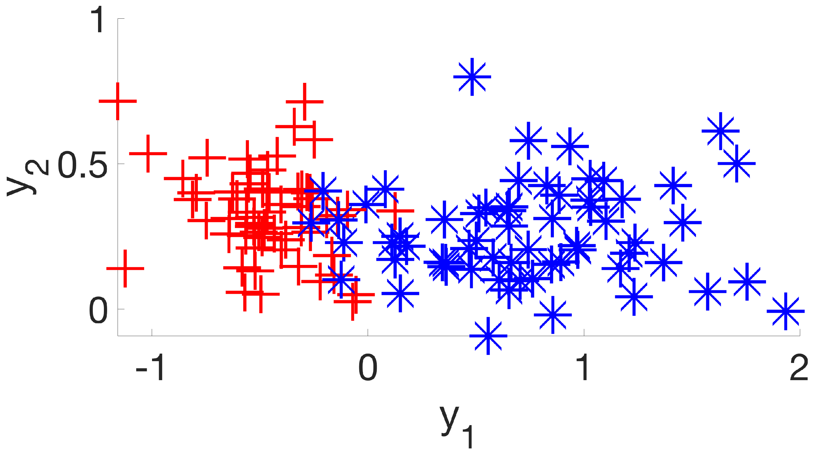
It is also interesting to see the final subset that will be forwarded to a classification method in Figure 10. Same-class individuals are much closer to one another, and cluster centers are much further apart from one another, just as Figure 2, Figure 3, Figure 4, Figure 5, Figure 6 and Figure 7 suggest. This is clearly a result of a higher silhouette coefficient.

The experiments indicate that the proposed method can improve the separability of data points, which can potentially enhance the accuracy of subsequent classification. In other words, the results suggests that the TSDR approach has the potential to improve classification by increasing the distinction between individuals.

The next section discusses how these findings impact accuracy, precision, recall, F1 score, and many other performance aspects. It is no secret that, considering the method heavily relies on optimization, it takes a longer time to run than another alternatives. Nevertheless, when dealing with real-life high dimensional spaces, that is a reasonable trade-off in search for a better result.

4. Experimental Results

The results of the proposed method, known as the TSDR approach, are presented in two parts in this section. Section 4.1 evaluates its classification performance on benchmark datasets, and Section 4.2 assesses its performance on a real-world application utilizing social media data.

The classification accuracy of the TSDR approach is compared to well-established algorithms. It is important to note that deterministic algorithms produce consistent outputs given the same inputs and machine state, while non-deterministic algorithms can produce varying outputs in the same circumstances [22].

The k-NN algorithm is a deterministic method that classifies based on the distances between a given sample and its k nearest neighbors. Its deterministic nature ensures consistent results given the same inputs. In contrast, the MLP is a non-deterministic algorithm, with the weights of its neurons initialized randomly and the calculation of errors unique to each iteration [23].

Comparing the efficiency of the TSDR approach with both deterministic and non-deterministic algorithms provides a comprehensive evaluation of the proposed method. Non-deterministic algorithms, such as the MLP, can be useful for finding approximate solutions when exact solutions are difficult to attain using deterministic methods.

While the parameterization of k-NN is straightforward, the same is not true for MLP, as it is a multilayer neural network that becomes more sensitive to the dataset. The appropriate number of neurons for each layer remains an area of uncertainty in the literature.

Next, we present some general guidelines for determining the number of neurons in the hidden layer of an MLP [24]:

• The number of neurons in the hidden layer should fall within the range between the size of the input layer and the size of the output layer.
• The number of neurons in the hidden layer should be equal to 2/3 of the size of the input layer, plus the size of the output layer.
• The number of neurons in the hidden layer should be less than double the size of the input layer.

In this study, the number of neurons in the single hidden layer of the MLP is arbitrarily determined by summing 2/3 of the number of features (in the input layer) and the number of labels (in the output layer). The only parameter yet to be defined is d, the number of desired dimensions in the output subset by the end of the first stage of the TSDR approach. As detailed in Section 3.2, the number of dimensions by the end of the second stage of the TSDR approach is solely determined by the number of classes in the original dataset.

Each of the methods (k-NN, MLP, LDA, and TSDR) were tested 100 times on various datasets. In each trial, a new training and test split was performed at fixed proportions of 60% and 40%, respectively. For each round, the TSDR was evaluated by varying the value of d from the total number of features minus one in the original dataset to the total number of classes plus one. Briefly, the classification performance for the following methods will be compared as follows:

• k-NN (deterministic method) on original dataset;
• MLP (non-deterministic method) on original dataset;
• LDA (non-deterministic method) on original dataset;
• TSDR discriminant function (as per Section 3.3 and Equation (15);
• k-NN on TSDR final subset;
• MLP on TSDR final subset;
• LDA on TSDR final subset.

4.1. Benchmark Datasets

The selected datasets, as listed in

Table 1. Selected benchmark datasets.

Dataset	Features	Labels	Individuals	k	Stage 1 d	Stage 2 d
cancer_dataset	9	2	{458, 241}	26	7	2
crab_dataset	6	2	{100, 100}	14	5	2
glass_dataset	9	2	{51, 163}	15	7	2
ovarian_dataset	100	2	{121, 95}	15	21	2

Note: d refers to the number of dimensions at the end of each stage.

, are well-suited to this application as they exhibit a range of attributes including varying numbers of labels and features. The distribution of instances among classes is also a critical aspect to consider when evaluating the performance of a method. High-dimensional datasets and simpler ones were both intentionally included in order to assess the impact of dimensionality reduction in both scenarios. The results shown in this section are those in which the value of d provided the highest level of accuracy for the classification methods. The parameter values of the methods for each dataset are also displayed in Table 1.

It was observed that the best classification results were obtained when the TSDR approach was used as a preprocessor on the datasets with the highest number of attributes, as demonstrated in

Table 2. Average accuracies for selected benchmark datasets.

Dataset	Original Dataset			TSDR Subset
	k-nn	MLP	LDA	k-nn	MLP	LDA	TSDRf
Cancer	95.63%	95.91%	95.84%	96.13%	96.27%	95.77%	96.27%
Crab	67.50%	96.75%	96.00%	92.25%	92.00%	93.50%	93.50%
Glass	90.12%	91.76%	93.88%	88.71%	91.29%	89.65%	91.76%
Ovarian	89.77%	86.51%	71.40%	91.63%	92.56%	91.63%	92.56%
Overall	85.75%	92.74%	89.28%	92.18%	93.03%	92.64%	93.52%

Note: The highest accuracy result for each dataset is highlighted in bold.

. The results indicate that dimensionality reduction has a positive impact on the final results. In certain cases, the accuracy achieved by the proposed built-in discriminator function for classification was even comparable to that of the MLP, which is widely recognized for its strong generalization ability.

As a matter of fact, considering that all datasets contain two classes and, therefore, that reduced subsets contain only two dimensions, the results are particularly positive because they possess comparable accuracy with much smaller datasets. In contrast, when the original datasets had low dimensionality, the classification methods performed better on the original datasets [25].

Another important performance indicator is the F1 score, calculated as the harmonic mean of precision (a measure of the number of correctly identified positive cases from all predicted positive cases) and recall (a measure of the number of correctly identified positive cases from all actual positive cases). This is a popular performance measure for classification when data are unbalanced, and provides a better measure of incorrectly classified cases than the accuracy metric [26].

As demonstrated in Table 2 and

Table 3. Average F1 scores for selected benchmark datasets.

Dataset	Original Dataset			TSDR Subset
	k-nn	MLP	LDA	k-nn	MLP	LDA	TSDRf
Cancer	95.29%	95.61%	95.52%	95.85%	96.06%	95.45%	95.98%
Crab	69.94%	96.80%	95.99%	92.33%	91.96%	93.75%	93.74%
Glass	86.24%	88.98%	91.35%	84.39%	88.20%	85.58%	88.93%
Ovarian	90.00%	86.95%	70.95%	91.54%	92.38%	91.81%	92.82%
Overall	87.36%	92.55%	88.45%	91.22%	92.07%	91.65%	92.71%

Note: The highest accuracy result for each dataset is highlighted in bold.

, overall, the use of the TSDR discriminator as a classifier leads to an improved accuracy and F1 score compared to the original datasets. Both k-NN and MLP show considerable increases in accuracy when the TSDR subsets are used for classification. However, a comprehensive evaluation of the proposed method should also consider the training time required to reach the final results [27].

It is important to note that the use of the TSDR approach requires additional computational time, as it involves solving two major optimization problems. However, the larger the dataset is, the smaller the overall time for classification becomes. For instance, the MLP requires an average of 67 s to train on the original ovarian_dataset, whereas it only requires an average of 0.1 s to train on the TSDR subset. Considering that it takes 31 s on average to obtain the final subset, the MLP can produce a result in no more than 32 s when using the reduced subset, which is much faster than the time required for the original dataset.

An analysis of the silhouette coefficient was also conducted in this study. The initial coefficient values for each dataset were calculated, as well for the subsets generated by the first (TSDR-1) and second (TSDR-2) stages of the proposed method. The results presented in

Table 4. Silhouette coefficients.

Dataset	Original	Stage 1	Stage 2
cancer_dataset	0.71	0.73	0.83
crab_dataset	0.01	0.40	0.70
glass_dataset	0.55	0.56	0.73
ovarian_dataset	0.46	0.35	0.65
Overall	0.40	0.49	0.71

show a significant improvement in the silhouette coefficient when comparing the original data to the subset utilized by the TSDR approach for classification, with all values more closely approaching 1, indicating that the clusters are more clearly separable and distinguishable from one another.

4.2. Social Media Dataset

To assess the effectiveness of a new algorithm, it is important to compare its accuracy against established methods using reference datasets. Once it passes this test, the next step is to test it in real-life applications with all the inherent randomness, overlap, and imbalances that only current data can provide. With this in mind, the TSDR was used to classify data from a social network.

Advances in technology have significantly improved the processing and storage capabilities of databases in recent years. The limitations of hardware and software have been overcome, making it easier to manage and expand large datasets. The increased processing power and the wider availability of cloud computing services have also made powerful technological resources more accessible. As a result, the combination of large databases and high-performance computers has made it possible to develop previously unimaginable applications [28].

Social networks, born from these technological advancements, are a treasure trove of information that is regularly mined by organizations seeking to better understand their consumers, competitors, and target audience. They provide insights into users’ interests and preferences, which can be used to understand and influence behavior. The applications are diverse, ranging from analyzing product or service receptivity, segmenting audiences for advertisements, or disseminating content to groups that are resistant to it [29].

Social networks have transformed society in the 21st century. The presidential elections in the United States and Brazil in 2016 and 2018, respectively, are strong examples of how digital strategists can guide public opinion, just as a conductor leads an orchestra. These professionals often use the services of data brokers, companies that aggregate and commercialize treated and enriched information from various sources, such as social networks, websites, and apps.

An example of the actions of these data brokers is the controversy surrounding the relationship between Cambridge Analytica (London, UK), a British political marketing company, and Facebook, where the data of over 50 million people was illegally collected via personality tests. The quiz, seemingly harmless, was able to quickly profile users based on information such as page likes and posts, obtaining not only the data of those who filled out the forms, but also the entire network of contacts of the participants. In this specific case, the data were allegedly used to outline the profile of the US population during Donald Trump’s presidential campaign in 2016, allowing for more efficient political advertising and targeted ads [30].

This was not the only controversy involving social networks during the same election. Russian interference, also widely reported, was subject to scrutiny by the authorities. A document published by the United States Senate Intelligence Committee concluded that Instagram was just as important as Facebook in influencing the results of the last presidential campaign.

The Internet Research Agency, a Russian company involved in digital influence operations on behalf of Russian political and commercial interests, sought to divide the American population using false information and adulterated content. The agency conducted more operations on Instagram than on any other social network, including Facebook, according to reports by the commission. From 2015 to 2018, there were 187 million interactions on Instagram, 77 million on Facebook, and 73 million on Twitter [31].

The classification of media engagement, which determines the level of audience reception based on its attributes, is a topic of significant interest. To this end, the application of the TSDR algorithm to a social media dataset was carried out. Prior to the classification process, the structure of the dataset must be defined and a construction process must be implemented.

In 2019, data from the social network Instagram were collected from 25 different users. For each of them, 2522 interactions were analyzed via an analysis of information from (up to) 12 of their last publications, repeating this same process for all users who interacted with them. A set of 6522 media records was built, belonging to 606 different users, enriched with information regarding their age, gender, hair color, and other cognitive data [32].

• Media width in pixels.
• Media height in pixels.
• Number of hashtags used.
• Length (in number of characters) of the caption.
• Number of males identified in the media.
• Average age of males identified in the media.
• Number of females identified in the media.
• Average age of females identified in the media.
• Gender of the owner of the media profile.
• Age of the owner of the media profile.
• Hair color of the owner of the media profile.

The dataset employed in the present study consisted of two distinct categories: “good engagement media” and “poor engagement media”. These categories were represented by 3,835 (58.8%) and 2687 (41.2%) media items, respectively. Engagement was determined as the ratio between the number of interactions (likes and comments) and the total number of followers. In the media industry, an engagement rate above 6% is commonly regarded as good, while values below that are considered poor. This classification serves as a starting point, although the engagement rate scale can be refined further [33].

The results of the original study, which utilized the same dataset as inputs for a multilayer perceptron (MLP), showed an accuracy of approximately 73% [34]. As per the results shown in

Table 5. Classification performance using Instagram dataset.

Measure	Original Dataset			TSDR Subset
	k-nn	MLP	LDA	k-nn	MLP	LDA	TSDRf
Accuracy	73.17%	74.78%	76.77%	75.91%	75.00%	77.11%	76.84%
F1 score	66.49%	70.34%	72.28%	71.34%	70.22%	72.55%	73.66%

Note: The best result for each measure is highlighted in bold.

and

Table 6. Parameters for Instagram dataset.

Measure	Original	Stage 1	Stage 2
Dimensions	11	8	2
Silhouette coefficient	0.12	0.19	0.40

, the application of the TSDR algorithm in the present study revealed a clear improvement, yielding an average accuracy of 77% using only two dimensions against 11 from the original research. This highlights not only the established premise, but also the efficacy of the proposed algorithm. Moreover, the accuracies for all methods were higher when using the TSDR subset for classification.

5. Conclusions

In this study, a two-stage dimensionality reduction (TSDR) method was proposed for data classification. The method involves two stages: extracting high-quality features by maximizing the pairwise separation probability and transforming the resulting subset into a reduced final space by maximizing the distance between the cluster centers and minimizing dispersion within the same class. The proposed method was tested on benchmark datasets and showed improved accuracy and F1 scores compared to the original datasets when used as a preprocessor or a classifier.

The results indicate that the higher the number of attributes is, the more the proposed method benefits from dimensionality reduction. The study also shows that the use of the TSDR approach leads to more distinguishable and separable clusters, as indicated by the significant improvement in the silhouette coefficient values. The use of the TSDR approach requires additional computational time, but the larger the dataset is, the smaller the overall time for classification becomes when compared to a simple neural network.

As the culmination of our research, it is essential to highlight the evolution of our work and the trajectory it has taken. While the current article delves into the successful application of TSDR and its comparison with various classifiers, we recognize that dimensionality reduction itself warrants an in-depth exploration of different methods and their comparative efficacy. As we plan to improve our existing proposal, our intention is to offer the research community a detailed examination of the nuances and strengths of various dimensionality reduction techniques, providing valuable insights for future endeavors in social data analysis.

This research also complements the results of a previous study on a social media dataset [32], which showed that the application of the TSDR algorithm improved the accuracy from 73% to 77%, even with a reduced dimension set. The method may also reduce the overall time required for classification. This result also highlights the effectiveness of the proposed algorithm in improving the performance of machine learning tasks. Moreover, it confirms the method’s potential regarding its application to real-life data.

In assessing the performance metrics of our classifier, it is crucial to contextualize the level of accuracy achieved. Social media datasets, particularly those derived from platforms like Instagram, are inherently dynamic, characterized by randomness and sparsity. The ability to attain a 77% accuracy in classifying such complex and diverse social data is a testament to the robustness of our two-state dimensionality reduction (TSDR) algorithm. It is essential to recognize the inherent challenges posed by the nature of social media content, where patterns and trends can emerge unpredictably.

Moreover, the noteworthy improvement from our previous work, where accuracy stood at 73%, underscores the efficacy of the enhancements introduced in this manuscript. This incremental progress represents a substantial step forward, and the level of accuracy achieved holds considerable significance within the intricate landscape of social data analysis. In fact, some even consider accuracies higher than 70% as human-level results [35]. As we navigate the intricacies of social media datasets, the pursuit of nuanced classification accuracy remains a continuous journey, and the strides made in this research contribute meaningfully to advancing state-of-the-art methods in the field.

The meaning and relevance of the results from a social standpoint are as important as the improved accuracies achieved with this novel approach. The world is witnessing mind-bending examples of how social networks are transforming life in society. The presidential election in the United States in 2016 is a solid example of how the work of digital strategists has been fundamental in driving public opinion, just as a conductor leads an orchestra.

Cambridge Analytica, a controversial political marketing company, paved the way for the development of highly effective political advertising on Facebook using approaches such as the one suggested by this paper. This resulted in the creation of assertive and precisely targeted ads for a specific candidate, who not only won the election but was later subjected to extensive scrutiny from the authorities following the revelations regarding the tactics used during the campaign [36].

Interestingly, this was not the only controversy involving the use of social media throughout the election: Russian interference, also widely reported by the media, was the target of scrutiny by the authorities. A document published by the United States Senate Intelligence Committee concluded that the actions taken on Instagram to influence the results of the last presidential campaign were just as important as those taken on Facebook.

The Internet Research Agency (Saint Petersburg, Russia), a Russian company involved in digital influence operations on behalf of its country’s political and commercial interests, which sought to divide the American population with false information and adulterated content, conducted more operations on Instagram than on any other social network, including Facebook, according to reports by the commission. There were 187 million interactions on Instagram, 77 million on Facebook, and 73 million on Twitter, according to data collected from 2015 to 2018 [37].

These numbers not only highlight the relevance of the proposed method, but also confirm the pertinence of the selected dataset. Moreover, these numbers makes one wonder how big the impact of similar approaches in the 2024 US presidential elections will be after eight years of technological advances following the infamous episode. Few changes have been made in terms of regulations, and the stage seems to be conducive for an even more impressive episode of these decisive approaches.

Conclusively, this work reveals that it is possible to classify whether or not a publication will receive a good amount of engagement with quite a high level of accuracy. The method can be used with handful of different data sources. It can also be used as a classifier or for dimensionality reduction within other machine learning algorithms. In future works, we intend to redesign the mathematical approach in order to adopt non-linear optimization in the algorithm’s second stage.