Distributed Action-Rule Discovery Based on Attribute Correlation and Vertical Data Partitioning

Abstract

The paper concerns the problem of action-rule extraction when datasets are large. Such rules can be used to construct a knowledge base in a recommendation system. One of the popular approaches to construct action rules in such cases is to partition the dataset horizontally (personalization) and vertically. Different clustering strategies can be used for this purpose. Action rules extracted from vertical clusters can be combined and used as knowledge discovered from the horizontal clusters of the initial dataset. The number of extracted rules strongly depends on the methods used to complete that task. In this study, we chose a software package called SCARI recently developed by Sikora and his colleagues. It follows a rule-based strategy for action-rule extraction that requires prior extraction of classification rules and generates a relatively small number of rules in comparison to object-based strategies, which discover action rules directly from datasets. Correlation between attributes was used to cluster them. We used an agglomerative strategy to cluster attributes of a dataset and present the results by using a dendrogram. Each level of the dendrogram shows a vertical partition schema for the initial dataset. From all partitions, for each level, action rules are extracted and then concatenated. Their precision, the lightness, and the number of rules are presented and compared. Lightness shows how many action rules can be applied on average for each tuple in a dataset.

1. Introduction

Every day, massive amounts of data are generated from a multitude of sources, from social media to scientific research. Analyzing and extracting useful insights from these vast datasets can be a daunting task, but action rules provide a powerful tool for identifying patterns and relationships within the data. They can help uncover hidden connections that may be invisible to human analysts. However, generating action rules efficiently for datasets with a large number of attributes remains a significant challenge.

Let us assume that objects in a dataset are described by a group of classification attributes and a single distinguished attribute called the decision attribute. Classification attributes can be further divided into stable and flexible. The values of flexible attributes, describing objects, can change in time, whereas values of stable attributes stay the same. Stable attributes are mainly used for the personalization of data mining results. Action rule discovery is a type of data mining method used to reclassify objects with respect to a decision attribute. The idea here is to identify sets of minimal changes in flexible attributes, describing certain objects, that would lead to a desired change in the decision value for these objects.

Action rules have been used to build a subclass of recommendation systems called knowledge-based recommendation systems. Domains of application include, among others, business (see [1,2,3]), healthcare (see [4,5,6]), music (see [7]), and art (see [8,9]). Next, we give a brief overview targeting some of these application areas.

The authors of [5] present a strategy to build a procedure graph for each medical procedure that takes place in a hospital. The procedure graph models sequences of consecutive procedures that follow the same initial procedure undertaken with a group of patients in a hospital. Data publicly available in the Florida State Inpatient Database (SID), which is a part of the Healthcare Cost and Utilization Project (HCUP) [10], were used for that purpose.

The paper also presents a collection of hierarchically structured recommendation systems used for decreasing the number of re-admissions to hospitals based on action rules extracted from the SID. To build these recommendation systems, patients in the SID were hierarchically partitioned into subgroups using their common characteristics as the filtering tool. This process is called the personalization of patients; it increases the predictability of the following procedures represented as nodes in the procedure graphs and also decreases the anticipated number of re-admissions. Here, action rules represent medical recommendations that can be used by physicians for placing a patient on the shorter, more successful, and safer procedure path.

Another work [11] presents a recommendation system for the surgical treatment of Parkinson’s disease. This kind of surgery is called deep brain stimulation (DBS). During DBS surgery, a set of three to five parallel-reading micro-electrodes are inserted into the patient’s brain. The electrodes are directed toward the expected location of the target nucleus, which is a small structure placed deep in the brain called the STN that does not show well in CT or MRI scans. At each desired depth, the reading electrodes record the electrophysiological activity of surrounding brain tissue. These electrodes advance until at least one of them passes through the nucleus, but it still requires an experienced neurologist/neurosurgeon to tell whether the recorded signal comes from the STN or not. The recommendation system presented in [11] answered this question with a confidence close to 100 percent. After such an electrode is verified, it is replaced by a permanent stimulating electrode.

Tarnowska and Ras [2] present a recommendation system based on knowledge (action rules) extracted from a sample dataset of customer feedback (around 300,000 records) concerning repair shops for caterpillar equipment covering 34 companies located in the US and Canada. Each record in the dataset represents a survey with features describing the company, the particular service assessed, and the customer surveyed. Feedback is represented by numerical scores in different areas and by additional notes in the free-form text. The Net Promoter Score (NPS) is used to partition the customers into three different groups: promoters, passive, and detractors. The goal is to extract action rules showing what minimal business changes are needed in the repair shops in order to change the customers’ status from passive to promoter, from detractor to passive, and from detractor to promoter. As already mentioned, action rules are composed of so-called stable attributes, flexible attributes, and target attributes. For stable attributes, the characteristics of a survey type and characteristics of a customer were chosen for the experimental setup. For flexible attributes, we chose benchmark questions from surveys, which represented areas of improvement in the customer satisfaction problem. The target attribute had three values: promoter, passive, and detractor.

In other work, the authors present a Basic Score Classification Database (BSCD), which describes associations between different scales, regions, genres, and jumps [7,12]. This database is used by a knowledge-based system to automatically index all submitted or retrieved pieces of music by emotion. Action rules extracted from the BSCD are used by a knowledge-based recommendation system to create solutions (automatically generated hints) that permit developers to manipulate a composition by retaining the music score while simultaneously varying the emotions it invokes. By score, we mean a written form of a musical composition.

Gelich and Ellinger [13] discuss a CO2 sensor network deployed in 16 equally divided parts of a classroom at UNC-Charlotte. Each part is equipped with one sensor node for CO2 concentration monitoring. Higher occupancy in the room triggers a higher value of CO2 concentration. Sensors in close proximity to people have higher CO2 readings. Personalized knowledge-based recommendation systems can be built to monitor indoor air quality inside the classroom and give recommendations on different strategies that can be followed to improve its air quality.

All of the above examples of knowledge-based recommendation systems show a variety of application domains where action rules can be successfully used. However, in many cases, action rules need to be discovered from large or very large datasets, not only those containing a large number of tuples but also a large number of attributes. Mining for action rules efficiently in such datasets can be a challenge. As the volume and complexity of data continue to grow, there is a critical need for methods that can efficiently discover action rules from large datasets.

To target this problem, we propose a new strategy for generating action rules based on the vertical partitioning of a dataset driven by correlations between its attributes. The idea is quite simple. We know, from rough sets theory that the more correlated attributes are in a dataset, the smaller its reducts are. Similarly, action rules should be shorter when discovered from datasets having correlated attributes. Therefore, instead of discovering action rules from a given dataset, we partition its attributes into clusters by treating the correlation as the distance measure. The more correlated the attributes are, the more close they are to each other in terms of distance. Our plan is to conduct hierarchical clustering and determine which level in the hierarchical tree provides the most effective attribute partition. Meaning, we iterate between each level to determine the optimal set of discovered action rules, defined by measures such as the number of rules, confidence, coverage, and lightness.

In this paper, we discuss our proposed method of distributed action rule discovery based on attributes correlation and vertical data partitioning and report on its performance as compared to other methods. Section 2 provides a background on recommendation systems and action rule discovery. In Section 3, we discuss a previous related work done for distributed action rule discovery and how our work differs. Section 4 provides all the information for the materials and methods. This includes detailed descriptions of both our proposed method and the random partitioning method we compare to. We also discuss the dataset used for experiments, data preprocessing steps, experimental parameters, and evaluation metrics used for the comparative analysis. In Section 5, we discuss the results found along with some example action rules. Finally, in Section 6, we discuss our conclusions and insights drawn from the study.

2. Background

2.1. Recommender Systems

For years, people have often recommended products or services through “word of mouth”. This highly social approach “pursued the principle of sharing an individual experience with others” [14]. Yet, with the development of the internet, we have now entered an era of “information explosion”. We live in a society where we are continuously retrieving information in all aspects of our lives [15]. Because of this information overload, it can be overwhelming to sift through it all ourselves. Therefore, it is essential to depend on technologies capable of filtering through available data and enabling the search for valuable insights [15]. Recommender systems are one such technology aimed at resolving this problem of information overload [14,15,16]. A comprehensive review paper covering this topic was published in 2019 (see [17]).

The goal of a recommender system is to suggest relevant items to the user. Recommender systems strive to anticipate the inclinations of a user or customer and furnish recommendations for additional resources or items that are probable to appeal to them. Specifically, recommender systems are designed to propose the most fitting products or services to specific users or businesses by forecasting a user’s curiosity in an item. This is done by utilizing data about analogous items, the users themselves, and the interactions between items and users.

Recommendation systems often collect information on users to generate a suitable recommendation of items [15]. This information can be in an explicit or implicit form of feedback [18]. Examples of explicit feedback include background information input by the user or item ratings the user provides through interaction. Implicit feedback is information the system infers based on the user’s behaviors, such as their navigation history or time spent on a certain page [18]. This information is used to create user profiles so that the system can better understand its users. After this information collection phase comes the learning phase, where learning algorithms are applied to “filter and exploit the user’s features from the feedback isinkaye2015recommendation. Finally, the recommendation phase combines the data and what has been learned to recommend or predict what items the user may like [15].

Depending on the data collected, various types of recommendation models can be applied. These models include:

• Collaborative Filtering: This method assesses items based on other users’ opinions [19]. This type of system utilizes the item ratings of many users to categorize them into groups based on their similarities. Items are then recommended to users based on those similarities.
• Content-Based Filtering: This technique is based on the user’s data itself, such as their inputted preferences or past interactions with the system, and the metadata associated with the items that exist in the system. With this system, users’ past preferences are usually mapped to predict their future preferences [15,19].
• Knowledge-Based: These systems determine the recommendations based on the user’s inputted requirements and the system’s knowledge about the items [15,19]. This method relies on external knowledge about items.
• Hybrid: These are systems that combine any of the above methods in ways to balance out each method’s strengths and weaknesses [19].

2.2. Action Rules

Action rules (or actionable patterns), first introduced by Ras and Wieczorkowska in [20], describe possible transitions of objects from one state to another with respect to a distinguished attribute called the decision attribute. Strategies for discovering them are divided into two types: rule-based and object-based. The rule-based approach consists of two main steps: (1) using a standard learning method to detect interesting patterns in the form of classification rules, association rules, or clusters, and (2) employing an automatic or semi-automatic strategy to inspect these results and derive possible action strategies. These strategies can provide insights into how the values of some attributes should be modified to move desirable objects into a desired group. The object-based approach assumes that actionable patterns are directly extracted from a database. Examples of rule-based strategies for extracting action rules are System DEAR (presented in [21]) and System DEAR2 (presented in [22]). Jan Rauch’s group has implemented these systems as modules of his LISP Miner software package (see [23,24,25]). Another example of a rule-based approach to action rules discovery is a strategy based on tree classifiers (see [26]). It should be mentioned here that the quality and quantity of action rules discovered heavily depend on the classification rules used in that process. To our knowledge, there is only one method based on discernibility functions in rough set theory that can discover all classification rules from a given dataset (see [27]). The more classification rules we have, the more action rules can be discovered. Object-based strategies for action rule mining have the same limitations—they do not discover all action rules [28]. An interesting concept is an action rules schema, which can be constructed directly from so-called action reducts. Action-rules schemas cover all action rules. Can we propose a strategy for generating all action rules from action-rules schemas?

Additional examples of strategies for action rules discovery can be found in publications by Kalanat (see [29,30]) and Dardzinska (see [31]). Action rules have been used in various domains, such as medical (see [5,6,32,33,34]) business (see [2,3,35,36]), music (see [7,12]), and art (see [8,9]). The rule-based approach has two main steps: (1) mining classification rules and (2) generating action rules from those classification rules. A classification rule $r_1$ is defined as a term:

$$r_1=[((A,a_1)\wedge (B,b_1)\wedge (C,c_1)\wedge (E,e_1))\Rightarrow (D,d_1)],$$

(1)

where, in the rule’s antecedent, $a_1$, $b_1$, $c_1$, and $e_1$ are attribute values associated with attributes A, B, C, E, correspondingly. Attribute value $d_1$, associated with attribute D, is a predicted target value called the consequent or the decision.

The support and confidence are calculated for each classification rule as a performance measure. The support is measured by the number of objects (or rows in the dataset) that match both the antecedent and consequent of a given rule. The confidence is the “ratio between” a given rule’s support and the total number of items that “satisfy [just] the antecedent” [37].

Action rules can be discovered directly from the dataset or constructed from classification rules. An action rule is defined as follows [20]:

$$r=[[a_1\wedge g_2\wedge (B,b_1\to b_2)\wedge (H,h_2)]\Rightarrow (D,d_1\to d_2)],$$

(2)

In the above, $a_1$ and $g_2$ are stable attributes, meaning they are attributes that do not change over time (their values cannot change). The next parts $(B,b_1\to b_2)$ and $(H,\to h_2)$ show the flexible attributes. These are the attributes that can change over time. The final piece, $(D,d_1\to d_2)$, is our consequent, the target value we wish to change. In the above example, it is stated that attribute A should equal $a_1$, attribute G should equal $g_2$, attribute B should change from $b_1$ to $b_2$, and attribute H should change from any value to $h_2$. If all of these happen, then a change in our consequent D from $d_1$ to $d_2$ is expected.

Let’s say we have two classification rules:

$$r_1=[(a_1\wedge b_1\wedge c_1\wedge e_1)\Rightarrow d_1],r_2=[(a_1\wedge b_2\wedge g_2\wedge h_2)\Rightarrow d_2].$$

(3)

Attributes A and G are stable, while B and H are flexible. If we have an object with features $a_1$, $b_1$, $c_1$, and $e_1$, the rule $r_1$ says that these four values impact the decision feature $d_1$ of that item. Assuming that the item also has a feature $(G,g_2)$ and we wish to change its decision feature to $d_2$, based on the info from $r_2$, we could change its value of B from $b_1$ to $b_2$ and the value of H to $h_2$. This would be expressed using the action rule [24]:

$$r=[[a_1\wedge g_2\wedge (B,b_1\to b_2)\wedge (H,\to h_2)]\Rightarrow (D,d_1\to d_2)].$$

(4)

Similarly to classification rules, we evaluate action rules using support and confidence, though calculated differently. In the above example, r is an action rule generated from the classification rules $r_1$ and $r_2$. The support of our action rule r is the same as $sup\left(r_1\right)$. The confidence of r is the product of both classification rules’ confidences: $conf\left(r_1\right)\times conf\left(r_2\right)$.

3. Related Works

The efficient extraction of action rules from large datasets has posed significant challenges to conventional models that analyze data in a non-distributed manner. Recognizing this limitation, there have been efforts to adopt a distributed approach to better handle the intricacies associated with larger volumes of data. This section provides an overview of such distributed approaches to action rule discovery, establishing the context for our proposed improvements.

Bagavathi et al. [38] introduces a distributed approach to extract action rules from large datasets. Their method emphasizes the data distribution phase, suggesting partitioning data into smaller granules both horizontally (across rows) and vertically (across attributes). Rules extracted from these vertical pairwise disjoint granules, which cover distinct attributes, are concatenated, thereby capturing some of the knowledge from the initial dataset. Similarly, Tarnowska et al. [35] propose another distributed method for action rule discovery using both horizontal and vertical partitioning. They employ Spark for horizontal partitioning, while their vertical approach randomly separates attributes. This method notably reduces the time required to discover action rules. However, a limitation lies in their combined study of both partitioning methods without isolation, making it unclear whether the benefits arise from horizontal partitioning, vertical partitioning, or a synergy of both.

While the above approaches offer a foundation for distributed action rule discovery methods, our work seeks to advance this further. We identify a potential limitation in the random nature of vertical data partitioning present in existing methods. Our contribution focuses on introducing a more logical and structured approach to vertical data partitioning. We propose using feature correlations as a distance measure in data partitioning, specifically for action rule discovery. This is a technique that, to the best of our knowledge, has not yet been explored. By doing so, we aim to enhance both the efficiency and the quality of the actionable patterns extracted from distributed datasets, distinguishing our work from existing methods.

4. Materials and Methods

4.1. Methods for Distributed Action Rule Generation

In this work, we propose a new method of action rule discovery based on attribute correlation and vertical data partitioning for datasets with many flexible attributes. Here, we will discuss the methodology in more detail.

4.1.1. Vertical Partitioning Based on Attribute Correlation

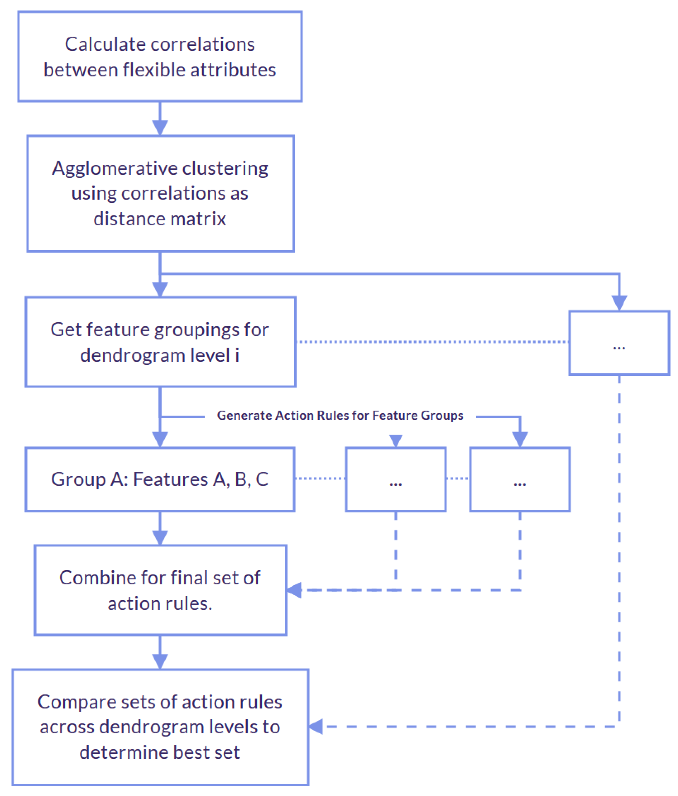
The process for this method are shown in Figure 1 and the steps include:

• Calculate the correlations between the flexible classification attributes in a given dataset.
• Perform agglomerative clustering on all of the flexible attributes using correlations among them as the distance measure, resulting in a dendrogram.
• Iterate through the different levels of the dendrogram, resulting in various sets of our flexible attributes clustered. Extract action rules for each cluster of flexible attributes, each one extended by the same stable attributes. Then, create all possible combinations, taking one action rule from each cluster and checking its support.
• Determine the best vertical partition of the dataset by comparing the F-scores of the sets of action rules discovered for each partition.

The first step is calculating the similarity between flexible attributes in a dataset. Similarity between attributes is calculated differently based on whether the attributes are continuous (numerical) or discrete (categorical). If both attributes are continuous, Pearson’s R correlation is used for that purpose. If both are discrete (categorical), we use Cramer’s V. If one attribute is continuous and the other is discrete, the Correlation Ratio is used.

Pearson’s correlation coefficient (r) is a way to measure the similarity between two attributes. It requires that both attributes are quantitative, normally distributed, and also specifically measure a linear relationship [39,40]. It is defined as follows:

$$Pearso{n}^{\prime }sR=\frac{n\sum xy-(\sum x)(\sum y)}{\sqrt{[n\sum x^2-{(\sum x)}^2][n\sum y^2-{(\sum y)}^2]}}$$

(5)

Cramer’s V measures the relationship between two nominal features, returning a 0 for no relationship or a 1 for a perfect relationship [39,40].

$$Crame{r}^{\prime }sV=\sqrt{\frac{X^2}{n\ast min(c-1,r-1)}}$$

(6)

where $X^2$ is the chi-square value, n is the sample size, c is the number of columns, and r is the number of rows.

We utilized the Dython Python (http://shakedzy.xyz/dython, accessed on 25 January 2024) library to calculate these associations given the attributes’ types (continuous or discrete). To calculate our distance matrix, we use the following:

$$DistanceMatrix=1-\frac{\left|associations\right|+1}{2}$$

(7)

We then performed agglomerative clustering using the distance matrix. Since all the attributes in our examples are categorical, only the Cramer’s V measure is used in the definition of a Distance matrix (by |D|, we mean the absolute value of D). We utilized the SciPy library (https://docs.scipy.org/doc/scipy/index.html, accessed on 25 January 2024) to perform the agglomerative clustering using single linkage and to create our dendrogram. Using this dendrogram, we iterated through to find the clusters at each level, resulting in various clusters of our flexible attributes. For example, if we have attributes {$A,B,C,D,E$}, we may get the following sets of clusters: (1) {A}, {B}, {C}, {$D,E$}, (2) {C}, {$D,E$}, {$B,A$}, and (3) {$D,E$}, {$B,C,A$}. Here, attributes D and E are closest to each other, B and A are next closest to each other, and then C is the closest to the {$B,A$} cluster. The last possible level would be to combine {$D,E$} and {$B,C,A$} into one cluster of {$A,B,C,D,E$}, but that is not what we need, but so we stop there. In other words, our aim is to break our flexible attributes into smaller groups to work with rather than working with them all at once. A single cluster of all attributes would defeat this purpose and is therefore not used.

We then generated action rules for each set of clusters. Clusters split the flexible attributes, and the stable attributes remained the same throughout. Using the example above, if we had two separate clusters {$D,E$} and {$B,C,A$}, we would generate action rules with the flexible attributes {$D,E$}, and then we would generate another set of separate action rules using the flexible attributes {$B,C,A$}. The stable attributes, consequent, and remaining parameters would remain identical for both. This work utilized the Python library developed by Sykora and Kliegr (see [37]) to generate action rules, implementing the rule-based strategy described by Ras and Wieczorkowska [20]. We will refer to this action rule generation method as Sykora’s package. Additionally, further experiments have been conducted using an alternative method for action rule discovery to facilitate comparative analysis. The details of this secondary action rule generation method are outlined in Section 4.1.2 and will be referred to as the RSES-based method.

Next, we concatenated the action rules by taking combinations of rules from each cluster. For each combination, we then checked its supporting objects and excluded any combinations that created action rules with a support of zero. Note that the stable attributes remained the same, but the flexible attributes differed across clusters.

As an example, cluster one may have the rule:

$$r_1=[(sex,male)\wedge (class,3\to 1)]\Rightarrow (survived,0\to 1)$$

(8)

Cluster two may have:

$$r_2=[(sex, male)\wedge (embarked, Southampton\to Cherbourg)]\Rightarrow (survived,0\to 1)$$

(9)

We would then try to form the combined rule:

$$r_3=[(sex, male)\wedge (embarked, Southampton\to Cherbourg)\wedge (class, 3\to 1)]\Rightarrow (survived, 0\to 1)$$

(10)

With this potential rule, we would then have to find the intersection of support sets for $r_1$ and $r_2$. If this intersection is empty, we cannot make $r_3$, and it would be excluded from the final set of action rules. Otherwise, it is added to our set of action rules for this particular partition.

To determine the optimal partition and the number of clusters to be used for rules extraction, we iterated through the newly created set of action rules for each cluster and evaluated its performance. Performance is evaluated using the F-score, defined by:

$$F-score\left(R\right)=2\ast \left(\frac{precision\ast recall}{precision+recall}\right)$$

(11)

Precision is defined by:

$$Precision\left(R\right)=\frac{\sum \{conf\left(r_i\right)\ast sup\left(r_i\right):i\in I\}}{\sum sup\left(r_i\right):i\in I}$$

(12)

where $conf\left(r_i\right)$ is the confidence of rule i, and $sup\left(r_i\right)$ is the support of rule i.

Recall, then, is defined by:

$$Recall\left(R\right)=card[\cup \{D_i:i\in I\}]/card\left(D\right),$$

(13)

where $card[\cup \{D_i:i\in I\}]$ is the cardinality (number of elements) of $\cup \{D_i:i\in I\}$. In other words, we found the percentage of all objects in D that are covered by R, our set of action rules. This definition of recall also takes into account the overlapping of domains—we want any object in overlapping domains to only be counted once. The set of action rules with the highest F-score determines the optimal partition of flexible attributes.

4.1.2. Random Partitioning

We compare the random vertical partitioning method to our initial proposed method (vertical partitioning based on attribute correlation). For random partitioning, instead of splitting based on correlation, it is fully random. This method was proposed by authors of [35], where they split the datasets vertically, by attributes, and extract action rules from multiple partitions. Similar to our method discussed previously, “once all parallel processes are complete, action rules from each partition are combined to yield the final recommendation of action rules” [35].

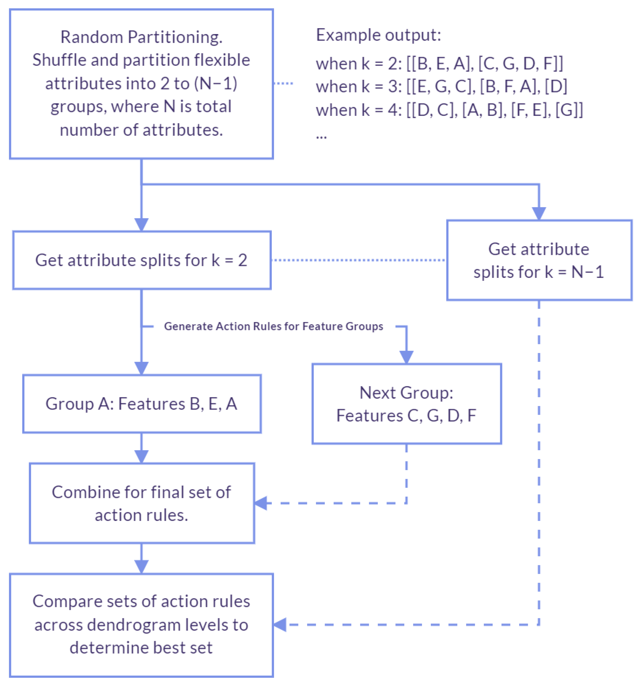
The process is illustrated in Figure 2 and the steps include:

• Generate multiple sets of groupings for flexible attributes, varying the number of groupings (N) from two to the total number of attributes (exclusive). In each set, shuffle the attributes randomly and divide them into k groups, where k ranges from 0 to N−1, creating diverse arrangements of the attributes. Store each set of groupings in a partition list.
• Iterate through each partition in the partitions list obtained in Step 1. Again, each partition is our set of flexible attributes randomly grouped. With each iteration, extract action rules for each group of flexible attributes. Then, create all possible combinations, taking one action rule from each group and checking its support.
• Determine the best partition of the dataset by comparing the F-scores of the sets of action rules discovered in each partition.

Again, for this method, splitting is done randomly. In our proposed method, splits are determined by correlation and clustering, not just randomly.

4.2. Additional RSES-Based Method for Action Rule Discovery

Again, our main experiments utilized the Python package developed by Sykora and Klieger (see [37]) for action rule discovery, adopting a rule-based approach to action rule mining.

We then utilized a secondary RSES-based action rule discovery method for comparison purposes. Initially, classification rules are generated using the Rough Sets Exploration System (RSES) tool. These rules are extracted from a dataset and typically represent patterns or associations between various attributes. Next, these classification rules outputted into a text file, are parsed and transformed into a structured format suitable for further analysis. This involved developing a parser that reads the text file, identifies the format of the rules, and converts them into a programmatically accessible format.

The classification rules are then categorized based on their decision attributes. In our case, they are grouped into “passive”, “promoter”, and “detractor” bins. For generating action rules, pairs of classification rules are compared, particularly focusing on rules that transition between different decision attribute values. Since our experiments focused on generating action rules reclassifying passive to the promoter, those are the bins we focused on.

Next, pairs of classification rules are compared (e.g., from ‘passive’ to ‘promoter’) to identify potential action rules. The comparison focuses on two types of attributes: stable attributes and flexible attributes. The method ensures that for any pair of classification rules being compared, their stable attributes are compatible (i.e., they have the same values or are absent in one of the rules). Flexible attributes are subject to change and are the focus of the action rules. This method looks for differences in flexible attributes between the pairs of rules to suggest possible actions.

Based on the comparison of classification rules, action rules are generated, suggesting changes in one or more flexible attributes that could lead to a transition from one decision class to another. The method takes into account various scenarios for each flexible attribute in the ruling pair, such as when an attribute is the same in both rules, when it differs, or when it’s present in one rule but not in the other. The action rules are formulated to recommend changes in attribute values that are hypothesized to result in the desired change in the decision attribute.

4.3. Experimental Setup

Our aim was to explore and compare the performance of the following methods: vertical correlation partitioning (our proposed method), random vertical partitioning, and no partitioning. In the case of no partitioning, action rules were generated from all of the given flexible attributes. The metrics used for evaluation include the following: the time to extract action rules and their count, the number of distinct objects covered by these rules, and the average number of identical objects included in the domains of all extracted action rules (referred to as the lightness).

The experiments were conducted on the UNC-Charlotte Orion research cluster. The cluster consisted of compute nodes equipped with Intel Xeon CPUs, with each node having 32 cores and 128 GB of RAM. The SLURM workload manager was utilized for job scheduling, resource allocation, and monitoring. The experiments were implemented using Python 3.8.5. We employed Ray as the parallel processing framework to accelerate the training of our machine learning models. Each experiment was executed on a single compute node, which featured 16 CPUs and 4 GB of memory per CPU. By harnessing the computational power of the cluster, we achieved significant reductions in the training time of our models.

4.3.1. Dataset Source and Background

One business metric used to evaluate customer experience is called the Net Promoter Score (NPS^®), a registered trademark of Satmetrix Systems, Inc., Redwood City, CA, USA (Bain and Company and Fred Reichheld). This score gauges the likelihood of customers recommending a company. Customers who are highly likely to recommend, scoring 9 or 10, are categorized as promoters. On the other hand, customers scoring 6 or below are referred to as detractors. Customers who fall in between are classified as passive, as they do not express strong advocacy or dissatisfaction.

For our experiments, we used the NPS (Net Promoter Score) dataset, which comprises customer feedback data collected on heavy equipment repair. We specifically chose this dataset to maintain consistency with related works, enabling us to offer a comparable assessment of our methodology. This also allowed us to adopt similar data pre-processing steps as those outlined in the related works. The dataset includes information from 38 companies and encompasses 340,000 customers across sites in the USA and Canada. Each customer survey is stored in a database, with each question (benchmark) represented as a feature in the dataset. The benchmarks consist of numerical scores ranging from 0 to 10, which indicate the quality of service provided. Examples of benchmarks include questions relating to job correctness, customer satisfaction, likelihood to refer, and more. The decision attribute in the dataset is labeled “PromoterStatus”, which classifies each customer as a promoter, passive, or detractor. The primary objective of the decision problem is to enhance customer satisfaction and loyalty, as measured by the Net Promoter Score. By applying action rules, the aim is to identify minimal sets of actions that can “reclassify” customers from “Passive” to “Promoter”, thus improving the NPS. For our experiments, we utilized surveys obtained from customers of four companies during the year 2015.

4.3.2. Data Preprocessing

Due to semantical inconsistencies in datasets representing 38 companies (resulting in low confidence in the extracted rules), we opted to select datasets from three companies for mining, labelling them as datasets A, B, and C. First, we followed several data preprocessing steps: (1) we removed columns based on a sparsity threshold, (2) we checked for correlations and removed redundant columns, (3) we handled null values, and (4) we categorized benchmarks into bins.

We first examined the sparsity of the benchmark columns and removed any columns that had 75% or more null values.

Next, we checked for correlations among all of the features using the pairwise correlation between numerical columns. Specifically, we used the Pearson correlation coefficient to measure the linear relationship between variables. If we identified any pairs of features with a one-to-one relationship, we removed one of the columns to eliminate redundancies.

We then handled null values based on the column. For any rows where the PromoterScore was null, we removed them since this attribute is our decision attribute, and its availability is necessary. For the benchmark features, we treated nulls as a separate category and created a new category called “No Response”.

This leads us to the next step of categorizing benchmark features into bins. In addition to treating null values as “No Response”, we assigned values between 0 and 4 (inclusive) to the category “Low”, values between 5 and 6 (inclusive) to “Medium”, values 7 and 8 to “High”, and values 9 and 10 to “Very High”.

4.3.3. Dataset Descriptions and Experimental Parameters

In our experiments, we utilized these three different subsets of the NPS dataset described in Section 4.3.1. Dataset A contained 542 rows, Dataset B contained 1279 rows, and Dataset C contained 661 rows. All three datasets were preprocessed and contained the same three stable attributes, named “division”, “survey type”, and “channel type”. Additionally, Dataset A had 11 flexible attributes, Dataset B had 10, and Dataset C had 10 as well. All flexible attributes in the dataset consisted of benchmarks taken from the discussed surveys. The consequent attribute used in all datasets is the “promoter status”. Possible values for the promoter status are “Detractor”, “Passive”, and “Promoter”. We conducted experiments for all datasets searching for action rules changing our consequent from “Passive” to “Promoter”. For all experiments, we applied a confidence threshold of 0.8 and a support threshold of 2 to filter rules extracted from this dataset.

4.3.4. Flexible Attribute Definitions and Vertical Correlation Partitioning Attribute Groupings

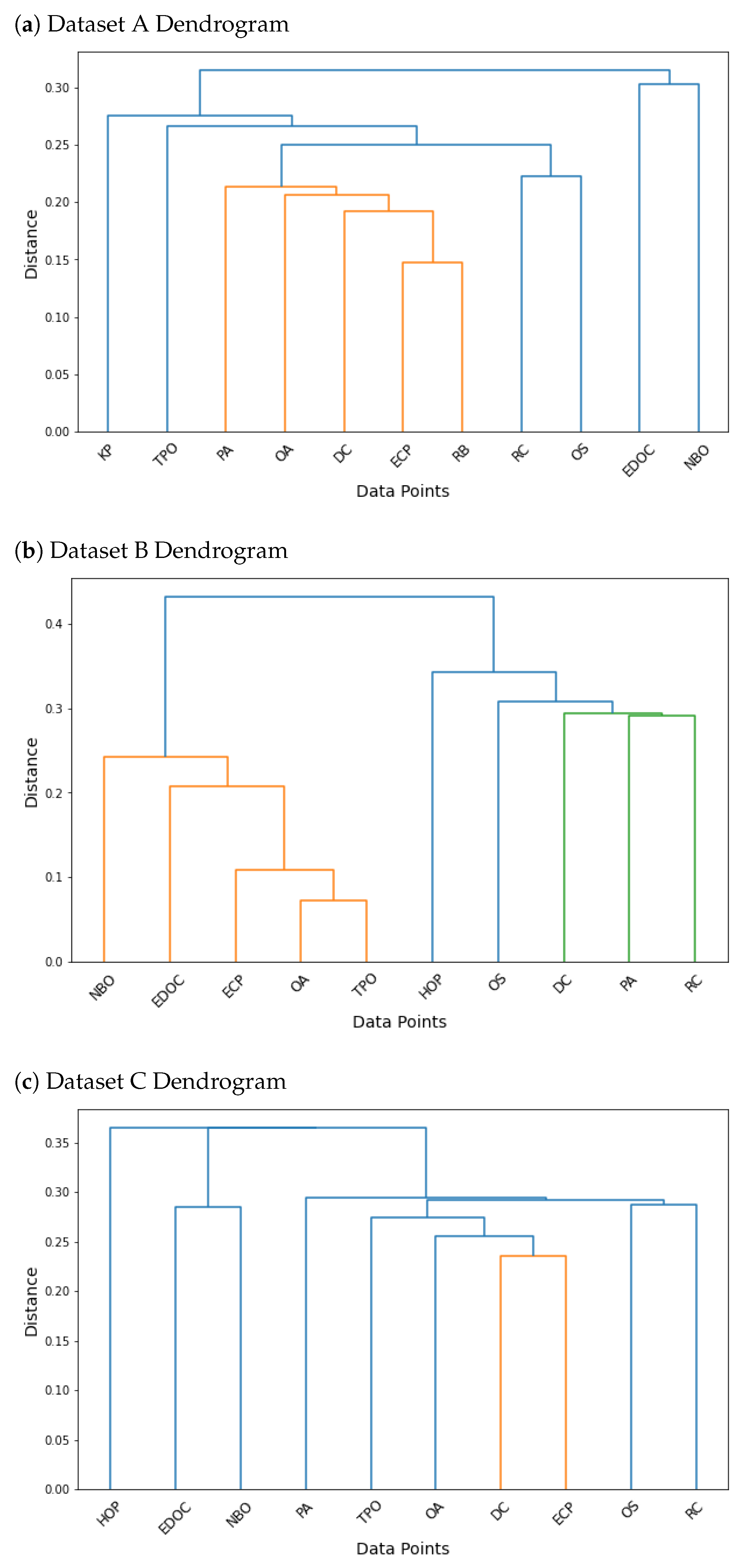
In our investigation, we concentrated on a set of flexible attributes, each of which contributed distinct insights to our vertical correlation partitioning methodology. These attributes, accompanied by their respective abbreviations and brief descriptions are shown in

Table 1. List of Attribute Abbreviations with Corresponding Names and Descriptions.

Abbreviation	Attribute Name and Description
DC	BenchmarkAllDealerCommunication: Evaluates communication effectiveness within the dealer network.
RC	BenchmarkAllLikelihoodtobeRepeatCustomer: Measures the likelihood of customer repeat business.
OS	BenchmarkAllOverallSatisfaction: Assesses overall customer satisfaction levels.
ECP	BenchmarkPartsEaseofCompletingPartsOrder: Gauges the ease of completing parts orders.
PA	BenchmarkPartsPartsAvailability: Examines component availability for order fulfillment.
TPO	BenchmarkPartsTimeitTooktoPlaceOrder: Measures the time taken for order processing.
EDOC	BenchmarkPartsExplanationofDeliveryOptionsCosts: Explores the elucidation of delivery options and related costs.
OA	BenchmarkPartsOrderAccuracy: Scrutinizes the accuracy of order processing.
NBO	BenchmarkPartsPromptNotificationofBackOrders: Examines the timeliness of back-order notifications.
KP	BenchmarkPartsKnowledgeofPersonnel: Assesses personnel knowledge about parts and their applications.
RB	BenchmarkReferralBehavior: Explores referral behaviors.
HOP	BenchmarkPartsHowOrdersArePlaced: Examines the methods of placing orders.

. Collectively, these attributes contributed to the dendrogram visualizations in Figure 3 that played a crucial role in determining flexible attribute groupings. These visualizations provide insights into the intricate relationships and patterns, enhancing our understanding of the vertical correlation partitioning process.

4.3.5. Evaluation Metrics

To facilitate the method comparison, we assessed various metrics including the run time (in seconds), the number of generated rules, precision, and the lightness. The run timerefers to the duration it takes for a method or process to complete its execution. In the context of our study, the run time is measured in seconds and indicates how long it takes for each method to run. This metric provides insights into the efficiency and computational speed of the method being evaluated. The computational efficiency of our method is paramount, especially when dealing with large datasets. By evaluating the run time, we ensure that our approach not only produces accurate results but also does so in a time-efficient manner, making it feasible for real-world applications.

The precision is previously defined in Equation (12) in Section 4.1.1. Precision provides information on the quality of the generated rules by reflecting both their support and confidence. A higher precision ensures that the rules are not only widely applicable but also reliable, making them invaluable for decision-making processes.

The number of generated rules represents the count of distinct rules produced by each method. In the context of this work, this metric reflects the richness and complexity of the rule set derived from each dataset. The quantity of generated rules can offer valuable information about the comprehensiveness and granularity of the rule-based system being analyzed. A greater number of rules offers a richer set of insights and actionable items. This directly corresponds with the lightness metric, further described below, wherein a higher value signifies more options for actionable insights.

The lightness is a ratio that serves as a measure of how evenly the coverage is distributed across the set of rules. By representing the average number of action rules that apply to each object, lightness helps distinguish between random and correlation-based partitioning. In business and healthcare, where actionable insights are vital, a lightness value between five and ten is considered ideal. The lightness for a generated set of action rules is defined in Equation (14) below:

$$\mathrm{Lightness}=\frac{\sum \mathrm{Coverage}\mathrm{of}\mathrm{each}\mathrm{action}\mathrm{rule}}{\mathrm{Coverage}\mathrm{of}\mathrm{entire}\mathrm{set}\mathrm{of}\mathrm{action}\mathrm{rules}}$$

(14)

The Coverage for each individual action rule is defined as the number of tuples or items that the action rule encompasses in the dataset. In other words, it represents the support of that particular action rule. The coverage for a set of action rules is determined by the unique support of all the rules within the set, shown in Equation (15) below.

$$\mathrm{coverage}\left(R\right)=\left|\bigcup _{r\in R}\mathrm{support}\left(r\right)\right|,$$

(15)

where R is a set of action rules, ⋃ represents the union operation, and $\left|·\right|$ represents the cardinality (or size) of a set. For example, if we consider rule ‘a’ with support for items indexed at [0, 1, 2, 3], and rule ‘b’ with support for items at [0, 1, 3, 4, 5], the aggregate coverage is 6. The individual coverage of rule ‘a’ is 4, while the individual coverage of rule ‘b’ is 5.

5. Results

The primary objective of this study was to address the following research questions: How does our novel approach to action rule generation compare with existing methods in terms of the time needed to generate rules for a given dataset? Additionally, how does the performance of our proposed method compare with that of the established approaches?

5.1. Comparative Insights

Table 2. Comparison of Method Performance Metrics Across Datasets and Feature Groupings.

Dataset	Method	Level	Time (Seconds)	Rules	Precision	Lightness
A	No Partition	1	1883.783	10.000	0.774	6.200
	Random	2	8.331	2.400	0.454	2.170
	Correlation		76.361	10.000	0.774	6.200
	Random	3	4.826	3.800	0.530	2.960
	Correlation		76.500	10.000	0.774	6.200
	Random	4	4.616	1.000	0.226	1.000
	Correlation		26.385	10.000	0.774	6.200
	Random	5	4.391	0.200	0.077	0.200
	Correlation		12.405	10.000	0.774	6.200
	Random	6	4.281	0.600	0.151	0.600
	Correlation		3.894	2.000	0.768	2.000
B	No Partition	1	966.701	19.000	0.797	10.477
	Random	2	5.970	9.600	0.786	6.367
	Correlation		5.657	14.000	0.789	7.277
	Random	3	3.930	6.100	0.615	4.029
	Correlation		4.124	14.000	0.789	7.277
	Random	4	3.618	3.500	0.466	2.311
	Correlation		4.117	7.000	0.765	3.873
	Random	5	3.533	1.900	0.544	1.467
	Correlation		3.884	1.000	0.779	1.000
C	No Partition	1	623.870	34.000	0.819	12.196
	Random	2	6.225	14.600	0.794	7.099
	Correlation		151.448	46.000	0.812	16.217
	Random	3	4.205	9.200	0.783	4.534
	Correlation		16.231	26.000	0.809	10.634
	Random	4	3.614	5.500	0.766	3.984
	Correlation		7.606	12.000	0.784	6.088
	Random	5	3.494	5.000	0.761	3.924
	Correlation		2.779	7.000	0.766	3.719
	Random	6	3.566	4.700	0.758	3.929
	Correlation		2.964	4.000	0.754	4.000
	Random	7	3.411	5.200	0.761	3.924
	Correlation		2.918	4.000	0.754	4.000
	Random	8	3.504	4.000	0.754	4.000
	Correlation		2.795	4.000	0.754	4.000
	Random	9	3.528	4.100	0.756	3.986
	Correlation		2.645	4.000	0.754	4.000

presents the results of two different vertical partitioning methods for action rule discovery along with the default (no vertical partitioning applied). These methods are applied to multiple datasets (A, B, and C). The methods evaluated are “No Partition”, representing the default approach with no vertical partitioning method, “Random”, which involves random vertical partitioning of flexible attributes, and “Correlation”, the proposed method utilizing correlation-based vertical partitioning through hierarchical clustering. The Random and Correlation methods iterate through different numbers of groupings of flexible attributes. The “Level” column illustrates this. For each dataset, method, and level, the table then shows the execution time (in seconds), the number of generated rules, the precision, and the lightness metrics. Note that the “Random” method results are averaged across ten different iterations. Methods for both “No Partition” and “Correlation” methods are only run once, as results are consistent each time. It can be observed that the “Correlation” method achieves varying performance across different datasets, outperforming both the “No Partition” and “Random” methods in some cases. These results highlight the importance of considering correlation-based vertical partitioning for improved performance in certain scenarios.

Our analysis of the ‘Random’ method and the correlation-based partitioning method on datasets A, B, and C revealed interesting insights into their respective performances. The ’Random’ method, with its random vertical partitioning of flexible attributes, demonstrated faster individual runs compared to the correlation-based method. However, achieving reliable and meaningful results required a relatively high number of extracted action rules, high confidence, and high lightness. In all three of these measures, the correlation-based method outperformed the random partitioning method.

The random-based method required extensive iterations (in our examples we used 10 iterations to get the averages). In contrast, the correlation-based partitioning method consistently produced results in each run without the need for extensive iterations. Although the correlation-based method generally exhibited slightly longer execution times than the ‘Random’ method, the time spent on obtaining averages was significantly reduced. The correlation-based partitioning method’s ability to generate consistent results enabled us to achieve reliable performance metrics in a single run, leading to a more efficient overall analysis.

Table 3. Comparison of Preliminary Performance Metrics for Secondary RSES-Based Action Rule Generation Method.

Dataset	Method	Level	Time (Seconds)	Rules	Precision	Lightness
A	No Partition	1	2726.625	1933.0	0.908	164.268
	Correlation	2	193.552	130.0	0.945	12.895
B	No Partition	1	58.101	36.0	0.843	12.958
	Correlation	2	20.484	22.0	0.855	5.099
C	No Partition	1	2019.907	4042.0	0.855	786.190
	Correlation	2	1158.997	602.0	0.893	70.293

shows the results of the action rule generation method described in Section 4.1.2. The RSES-based action rule generation method produced significantly more rules compared to the approach utilizing Sykora’s package. For instance, in Dataset A, the RSES-based method extracted 1933 rules compared to only 10 rules by Sykora’s package. However, this increase in rule generation came at the cost of increased execution time, as seen in the longer runtime for the RSES-based method for Datasets A and C. Extracting action rules using the RSES-based method was faster for Dataset B. Notably, for Dataset A when employing the vertical partitioning method, the execution time was 193.552 s at level 2. However, with the correlation vertical partitioning, we observed faster runtimes.

Our findings here underscore the importance of considering not only execution time but also the quality, and consistency of results when evaluating vertical partitioning methods for action rule discovery tasks. The correlation-based partitioning’s capacity to yield reliable outcomes in a single run, a relatively large number of extracted action rules, their high confidence, and high lightness (in comparison to “random” methods) present a preferable alternative, particularly when dealing with large datasets or applications where the quality and diversity of discovered action rules are essential.

5.2. Individual Action Rules

In this section, we present several examples of the generated action rules. Our focus is specifically on the rules generated for Dataset C and at level 2. We chose this particular level because it yielded the most extensive set of rules using the vertical correlation partitioning method. When referring to the dendrograms in Figure 3, we can observe the feature groupings established by the flexible vertical correlation partitioning method.

5.2.1. Illustrating Vertical Correlation Method Combinations

In this section, we focused on utilizing the Vertical Correlation Method to generate action rules to illustrate instances of action rules being generated within one dendrogram level and making their combinations. This iteration employed a confidence threshold of 50% and a support threshold of two for rule generation. Our analysis centered on Dataset C and exploreed results obtained from examining “Level 5” of the dendrogram. Refer to Figure 3 for the Dataset C dendrogram and how flexible attributes were clustered. Within this level, distinct clusters emerged, with attributes such as OA, DC, TPO, and ECP forming one cluster, and OS and RC forming another. By showcasing these specific configurations, we aim to offer insights into the patterns and relationships revealed by the vertical correlation approach.

Example 1.

In one of the instances of generated action rules, we examined one rule at level 5. This rule, shown in Equation (16) reads as follows: if the division attribute equals “parts” and simultaneously experiences changes in the TPO attribute from “high” to “very high”, changes in ECP from “high” to “very high”, and changes in RC from “high” to “very high”, the resulting implication is a shift in PromoterStatus from “Passive” to “Promoter”. In other words, we want to increase the company’s ratings for the time it took to place the parts order, the ease of completing the parts order, and the customer’s rating to be a likely repeat customer. If all of these change from high to very high, we can infer a change in the promoter status from passive to a promoter. This rule had a support of 15 and a confidence of 0.755.

$$\begin{array}{c}\hfill (Division,\mathrm{parts})\wedge (TPO,\mathrm{high}\to \mathrm{very}\mathrm{high})\wedge (ECP,\mathrm{high}\to \mathrm{very}\mathrm{high})\\ \hfill \wedge (RC,\mathrm{high}\to \mathrm{very}\mathrm{high})\\ \hfill \Rightarrow (PromoterStatus,\mathrm{Passive}\to \mathrm{Promoter})\end{array}$$

(16)

This rule represented a synthesis of two distinct rules from each of the clusters at this level. As we can see in our earlier Figure 3, one cluster for Dataset C at level 5 consists of the flexible attributes OA, DC, TPO, and ECP while the other consists of OS, and RC. The first rule, shown in Equation (17) entails: “if division = parts, TPO changes from high to very high, ECP changes from high to very high, the implication is a transition in promoter status from passive to promoter”. This first rule had a support of 22 and a confidence of 0.499. The second rule, shown in Equation (18), contributing to this combination is: “if division = parts and RC changes from high to very high, we infer a change in promoter status from passive to promoter”. This rule had a support of 39 and a confidence of 0.7211.

$$\begin{array}{c}\hfill (Division,\mathrm{parts})\wedge (TPO,\mathrm{high}\to \mathrm{very}\mathrm{high})\wedge (ECP,\mathrm{high}\to \mathrm{very}\mathrm{high})\\ \hfill \Rightarrow (PromoterStatus,\mathrm{Passive}\to \mathrm{Promoter})\end{array}$$

(17)

$$\begin{array}{c}\hfill (Division,\mathrm{parts})\wedge (RC,\mathrm{high}\to \mathrm{very}\mathrm{high})\\ \hfill \Rightarrow (PromoterStatus,\mathrm{Passive}\to \mathrm{Promoter})\end{array}$$

(18)

Example 2.

In this second example, also from level 5, our rule is shown in Equation (19). It shows that if our division is in parts, the accuracy of order processing (OA) changes from high to very high, the communication effectiveness within the dealer network (DC) changes from high to very high, and the likelihood of customer repeat business (RC) changes from high to very high, it implies a change in our promoter status from a passive to a promoter. This rule had a support of 11 and a confidence of 0.755.

$$\begin{array}{c}\hfill (Division,\mathrm{parts})\wedge (OA,\mathrm{high}\to \mathrm{very}\mathrm{high})\wedge (DC,\mathrm{high}\to \mathrm{very}\mathrm{high})\\ \hfill \wedge (RC,\mathrm{high}\to \mathrm{very}\mathrm{high})\\ \hfill \Rightarrow (PromoterStatus,\mathrm{Passive}\to \mathrm{Promoter})\end{array}$$

(19)

The rules that were combined to form the above one are shown in Equations (20) and (21). The first one describes that if our division is in parts and we change both OA and DC from high to very high, we then infer an increase in promoter status from passive to promoter. This rule had a support of 17 and a confidence of 0.507. The second rule states that if our division is in parts and we increase RC from high to very high, we also imply an improvement in promoter status from passive to promoter, with a support of 39 and confidence of 0.721.

$$\begin{array}{c}\hfill (Division,\mathrm{parts})\wedge (OA,\mathrm{high}\to \mathrm{very}\mathrm{high})\wedge (DC,\mathrm{high}\to \mathrm{very}\mathrm{high})\\ \hfill \Rightarrow (PromoterStatus,\mathrm{Passive}\to \mathrm{Promoter})\end{array}$$

(20)

$$\begin{array}{c}\hfill (Division,\mathrm{parts})\wedge (RC,\mathrm{high}\to \mathrm{very}\mathrm{high})\\ \hfill \Rightarrow (PromoterStatus,\mathrm{Passive}\to \mathrm{Promoter})\end{array}$$

(21)

Here, we delved into the application of the Vertical Correlation Method to generate actionable insights through synthesis of action rules. By using a confidence threshold of 50% and support threshold of two, we specifically explored the patterns emerging at level 5 of the dendrogram within Dataset C. Through this, we provided specific instances of how action rules were generated for different clusters of flexible attributes and then combined together. These insights help contribute to a deeper understanding of the interconnections within the dataset, revealing potential strategies for enhancing the PromoterStatus transitions.

5.2.2. Vertical Correlation Partitioning Method

For Dataset C and Level/Groupings 2, this method generated 46 rules with a precision of 0.812 and lightness of 16.217.

Some action rules generated by this method are as follows:

$$\begin{array}{c}\hfill (Division,\mathrm{parts})\wedge (OS,\mathrm{high}\to \mathrm{very}\mathrm{high})\wedge (RC,\mathrm{high}\to \mathrm{very}\mathrm{high})\\ \hfill \Rightarrow (PromoterStatus,\mathrm{Passive}\to \mathrm{Promoter})\end{array}$$

(22)

$$\begin{array}{c}\hfill (Division,\mathrm{parts})\wedge (RC,\mathrm{high}\to \mathrm{very}\mathrm{high})\wedge (PA,\mathrm{high}\to \mathrm{very}\mathrm{high})\\ \hfill \Rightarrow (PromoterStatus,\mathrm{Passive}\to \mathrm{Promoter})\end{array}$$

(23)

$$\begin{array}{c}\hfill (Division,\mathrm{parts})\wedge (RC,\mathrm{high}\to \mathrm{very}\mathrm{high})\wedge (TPO,\mathrm{high}\to \mathrm{very}\mathrm{high})\\ \hfill \Rightarrow (PromoterStatus,\mathrm{Passive}\to \mathrm{Promoter})\end{array}$$

(24)

$$\begin{array}{c}\hfill (Division,\mathrm{parts})\wedge (RC,\mathrm{high}\to \mathrm{very}\mathrm{high})\wedge (EDOC,\mathrm{no}\mathrm{response}\to \mathrm{very}\mathrm{high})\\ \hfill \Rightarrow (PromoterStatus,\mathrm{Passive}\to \mathrm{Promoter})\end{array}$$

(25)

5.2.3. Random Partitioning Method

For Dataset C and Level/Groupings 2, this method generated an average of 3.686 rules with a precision of 0.460 and lightness of 2.538, averaged across 10 iterations. Examples of rules from one iteration returning 22 different rules include:

$$\begin{array}{c}\hfill (Division,\mathrm{parts})\wedge (RC,\mathrm{high}\to \mathrm{very}\mathrm{high})\wedge (OS,\mathrm{high}\to \mathrm{very}\mathrm{high})\\ \hfill \Rightarrow (PromoterStatus,\mathrm{Passive}\to \mathrm{Promoter})\end{array}$$

(26)

$$\begin{array}{c}\hfill (Division,\mathrm{parts})\wedge (PA,\mathrm{high}\to \mathrm{very}\mathrm{high})\wedge (RC,\mathrm{high}\to \mathrm{very}\mathrm{high})\\ \hfill \Rightarrow (PromoterStatus,\mathrm{Passive}\to \mathrm{Promoter})\end{array}$$

(27)

$$\begin{array}{c}\hfill (Division,\mathrm{parts})\wedge (RC,\mathrm{high}\to \mathrm{very}\mathrm{high})\wedge (EDOC,\mathrm{high}\to \mathrm{very}\mathrm{high})\\ \hfill \Rightarrow (PromoterStatus,\mathrm{Passive}\to \mathrm{Promoter})\end{array}$$

(28)

Another iteration provides 13 rules, including those shown in Equations (26) and (27), but did not have the rule shown in Equation (28). One rule unique to this iteration is:

$$\begin{array}{c}\hfill (Division,\mathrm{parts})\wedge (DC,\mathrm{high}\to \mathrm{very}\mathrm{high})\wedge (OS,\mathrm{high}\to \mathrm{very}\mathrm{high})\\ \hfill \wedge (PA,\mathrm{high}\to \mathrm{very}\mathrm{high})\Rightarrow (PromoterStatus,\mathrm{Passive}\to \mathrm{Promoter})\end{array}$$

(29)

Note that we have pulled some rules for examples from the random iterations that had a higher number of generated rules.

6. Discussion and Conclusions

This paper addresses action rule extraction from large datasets, a task that can be approached using two methods: rule-based and object-based. In the rule-based approach, the first step involves discovering classification rules, followed by examining their pairs to check if action rules can be constructed. There are known software packages available for generating these rules, such as Lisp-Miner [24] and SCARI [37]. However, a limitation of current action rule discovery packages, including Lisp-Miner and SCARI, is that they generate only small subsets of all classification rules, resulting in a much smaller set of action rules. Consequently, achieving sufficient coverage for the resulting action rules classifiers becomes problematic. Moreover, when the number of discovered action rules is limited, their lightness decreases. By lightness, we refer to the average number of action rules that support objects in a dataset. For instance, if the lightness is two, only two action rules can be applied to reclassify objects. It can happen that both of these options are either too costly or, for various reasons, unacceptable to users. Therefore, in such cases, they can not be applied. In the domain we tested, business owners expected to have a lightness measure of about ten. If the lightness measure exceeds this value, they prefer to see the top ten best action rules (using the visibility measure [36]).

In the object-based approach, action rules are discovered directly from a dataset, resulting in a larger number of rules than following a rule-based approach. However, we are unaware of any software package discovering almost all action rules. One possibility is system ARED, which generates action schemas covering all action rules (see [41]). The question arises as to how to generate all or almost all action rules from these action schemas. Many datasets are large or very large. One potential strategy for extracting action rules from them is to begin by splitting the dataset vertically and/or horizontally, extracting action rules from these splits, and subsequently merging them.

In this paper, we focused on knowledge discovery methods based on splitting dataset schemas into vertical clusters, comparing our proposed correlation vertical partitioning to both random vertical partitioning and the base (no partitioning) method. Our comprehensive evaluations on subsets of the NPS dataset highlight crucial differences between these methodologies. Specifically, the results in Table 2 demonstrate that the random partition generally yields fewer action rules compared to methods based on attribute correlation.

Furthermore, when examining metrics such as precision and lightness across the datasets, methods grounded in attribute correlations consistently outperformed those based on random vertical partitioning, producing results comparable to the base method. For instance, the precision achieved using the correlation-driven approach exhibited either a notably higher or comparable precision compared to its random counterpart. This trend was similarly observed in terms of lightness across all datasets, indicating the broader applicability of the correlation-based technique.

High lightness, as observed in our results, indicates the presence of a more extensive set of action rules, and therefore options for a user to explore. From a business standpoint, this is invaluable. Business stakeholders often require diverse options to weigh against varying costs, safety concerns, and potential outcomes of action rule suggestions. The fact that correlation-based partitioning offers this versatility, coupled with its consistent performance and reduced need for iterative runs, establishes it as a preferred method, particularly in scenarios with extensive datasets or where the quality and diversity of discovered action rules are crucial.

In conclusion, our research highlights the advantages of leveraging attribute correlations in vertical partitioning for action rule discovery. Beyond just considering execution time, it is important to account for the quality, consistency, and business applicability of results, areas where correlation-driven partitioning excels.