Multi-Scale Rolling Bearing Fault Diagnosis Method Based on Transfer Learning

Abstract

Confronting the challenge of identifying unknown fault types in rolling bearing fault diagnosis, this study introduces a multi-scale bearing fault diagnosis method based on transfer learning. Initially, a multi-scale feature extraction network, MBDCNet, is constructed. This network, by integrating the features of vibration signals at multiple scales, is dedicated to capturing key information within bearing vibration signals. Innovatively, this study replaces traditional convolution with dynamic convolution in MBDCNet, aiming to enhance the model’s flexibility and adaptability. Furthermore, the study implements pre-training and transfer learning strategies to maximally extract latent knowledge from source domain data. By optimizing the loss function and fine-tuning the learning rate, the robustness and generalization ability of the model in the target domain are significantly improved. The proposed method is validated on bearing datasets provided by Case Western Reserve University and Jiangnan University. The experimental results demonstrate high accuracy in most diagnostic tasks, achieving optimal average accuracy on both datasets, thus verifying the stability and robustness of our approach in various diagnostic tasks. This offers a reliable research direction in terms of enhancing the reliability of industrial equipment, especially in the field of bearing fault diagnosis.

1. Introduction

Bearing fault diagnosis is a key technology in terms of enhancing the performance, prolonging the lifespan, and ensuring the safe and stable operation of rotating machinery equipment [1,2]. Bearings, as critical components in rotating machinery, support the load on rotating shafts and ensure smooth operation. Faults or damage in bearings can not only degrade the equipment’s performance but also lead to severe accidents and equipment downtime and potentially cause the loss of life and property. Therefore, it is crucial to precisely diagnose bearing faults with modern sensor technology and data analysis methods. This approach not only prevents faults but also optimizes maintenance schedules, improves equipment efficiency, and reduces maintenance costs and downtime [3,4,5].

Current bearing fault diagnosis methods encompass those derived from traditional machine learning [6,7,8] and deep learning [9,10,11]. Among them, deep learning models have been widely studied and applied because of their ability to automatically extract useful features from complex data. Chen et al. proposed a deep learning fault diagnosis method based on cyclic spectral coherence diagrams and convolutional neural networks, which improved the identification of rolling bearing faults, but all fault types appeared in the training set [12]. Arellano-Espitia et al. demonstrated the advantages of applying deep learning technology for fault diagnosis in different bearing technologies [13]. Meanwhile, Zhao et al.proposed a hybrid deep autoencoder method for bearing fault diagnosis, capable of classifying both existing and new faults, thereby improving the accuracy [14]. However, these studies did not consider the approaches’ applicability across different operational conditions. In real industrial environments, the training and testing data may be obtained under different operational conditions, such as varying loads and speeds, leading to domain drift and consequently low fault diagnosis accuracy [15,16]. In other words, changes in working conditions cause variations in the bearing signal features across the source and target domains, which can affect the reliability of common methods. Moreover, acquiring sufficient vibration signal data and corresponding labels to train models for specific health states is challenging. Thus, bearing fault diagnosis under different working conditions is of significant practical importance.

Transfer learning, as a cutting-edge machine learning technique, offers an effective solution for bearing fault diagnosis challenges under varying working conditions [17,18]. The core idea of this technique is to leverage existing knowledge and data to effectively combine information from both the source and target domains, enabling more precise bearing state diagnosis under new conditions. The advantages of transfer learning are not only reflected in improving the diagnostic accuracy but also in reducing the cost of data collection and labeling and enhancing the efficiency of model training. This is because it allows the transfer of valuable knowledge from the source domain to the target domain, thus better addressing challenges under varying operational scenarios. Asutkar et al. [19] proposed an efficient transfer learning strategy, fine-tuning the trainable parameters with target domain datasets for domain generalization in mechanical fault diagnosis. Zhong et al. [20] introduced a lightweight convolutional neural network that combines transfer learning and self-attention integration for bearing fault diagnosis, highlighting the potential of transfer learning in improving the diagnostic accuracy. Zhao et al. [21] utilized a Gaussian prior distribution to construct a common feature space and designed a conditional weighting strategy to quantify the similarity between different source and target domains. An et al. [22] proposed an adversarial domain adaptation network based on contrastive learning, offering a solution for bearing fault diagnosis under different conditions and reducing misclassification. Zhu et al. [23] introduced a generative convolutional neural network, using multi-kernel MMD to enhance the feature transferability. Wang et al. [24] constructed a multi-scale deep intra-class adaptation network and developed a multi-scale feature learner, validating the model’s effectiveness through extensive comparative experiments. Shao et al. [25] proposed a method based on transfer convolutional neural networks and thermal imaging technology for the intelligent diagnosis of rotating bearing systems under different working conditions, overcoming training issues in traditional CNNs by introducing random pooling and activation functions and adapting the source domain parameters to the target domain through transfer learning.

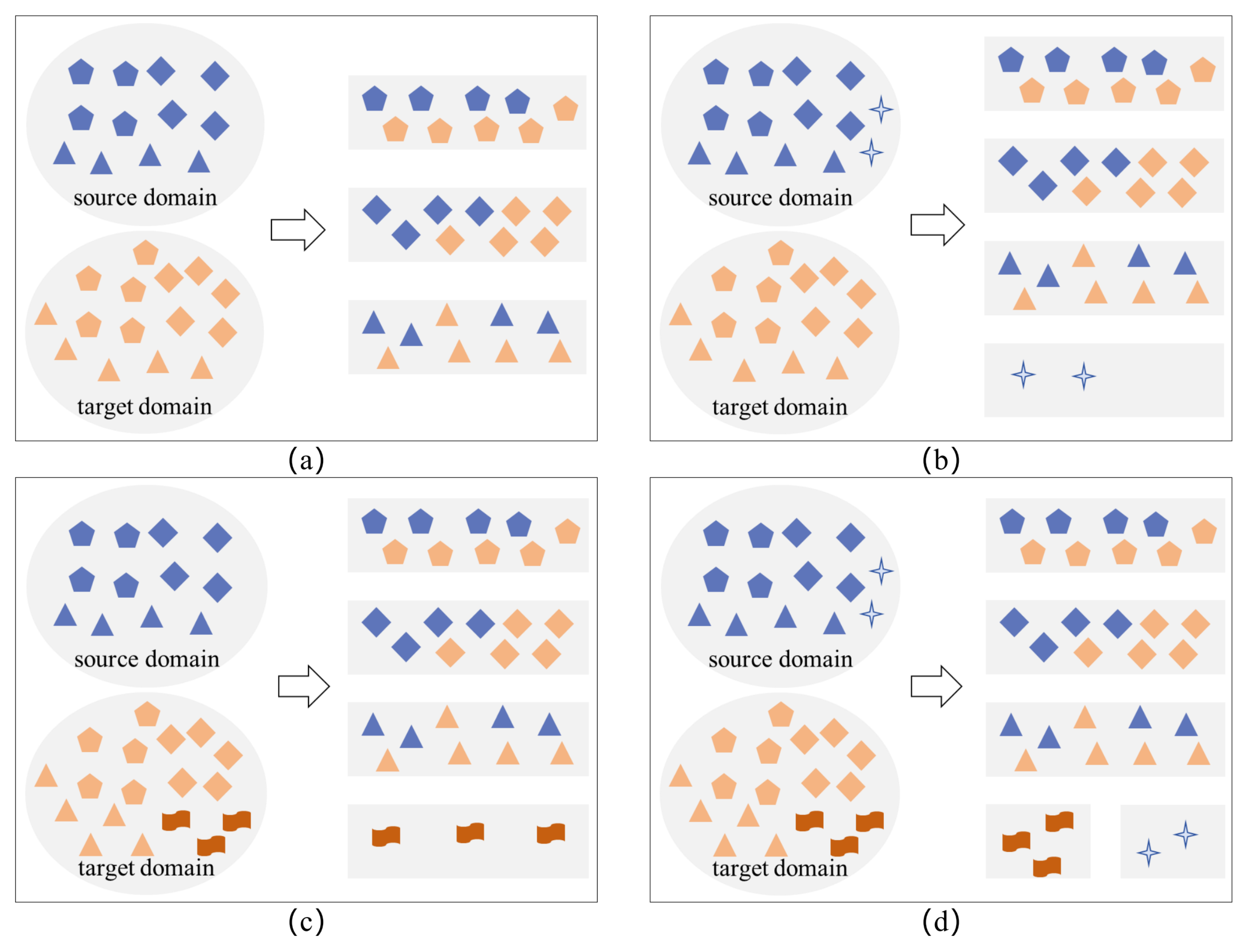
Although the aforementioned transfer learning and deep learning methods for bearing fault diagnosis have shown excellent performance under specific conditions, they typically rely on a key assumption: all fault types in the target domain are represented in the source domain, meaning that the source domain data cover all fault types in the target domain. However, in actual industrial applications, especially considering the safety of equipment operation, it is difficult to operate bearings under all potential fault states to collect data, leading to a lack of fault data for all types. Therefore, the fault type matching relationship between the source and target domains can actually be divided into four different scenarios, as shown in Figure 1. Figure 1a indicates that the fault categories in the source and target domains are the same, but the operating conditions may not be identical; Figure 1b shows that the target domain’s fault types are a subset of those in the source domain. These two scenarios are ideal but difficult to meet in real-world settings. Figure 1c implies that the fault categories from the source domain fall within the range of the target domain’s, meaning that there are additional fault types in the target domain not present in the source domain. Figure 1d shows that the source and target domains have both the same and specific categories. Clearly, the scenarios in Figure 1c,d better represent the most common scenarios in practical industrial applications.

Recent research has made significant progress in addressing the issue of effectively recognizing new fault types that are limited by the constraints of the source domain. Zhao et al. [16] proposed a bearing fault diagnosis method based on a dual adversarial network, incorporating an auxiliary domain discriminator to assess the similarity of individual target samples. Yu et al. [26] examined the problem of open-set fault diagnosis and proposed the BWAN model for COSFD, which assigns greater weight to shared classes during feature alignment and less weight to outlier classes. Liu et al. [27] introduced a novel OSFD method, which relaxes the constraint of identical label spaces between the source and target domains, designs a regularization method to convert open sets into pseudo-closed sets, and introduces a sample-level weighting mechanism, demonstrating the effectiveness of this fault diagnosis approach through experiments. These methods have enabled notable progress in addressing the issue of recognizing new fault types in target tasks that are limited by the constraints in source task data. They offer valuable research directions for this issue. However, there remains potential for additional enhancements in recognition accuracy.

Building on the aforementioned studies, this paper presents research on bearing fault diagnosis methods based on transfer learning, aiming to further explore and improve the issue of low recognition accuracy for new fault types in target tasks due to limitations in source task data. The key contributions of this paper can be summarized as follows.

• Construction of a multi-scale bearing fault diagnosis model. This study constructs a multi-scale bearing fault diagnosis model based on transfer learning. Through transfer learning strategies, this model effectively utilizes knowledge gained from related but different tasks. This approach grants the model stronger generalization capabilities when dealing with new fault types. In particular, the model is capable of addressing potential differences in fault types between the source and target domains, thereby improving the diagnostic accuracy in target operating conditions.
• Design of a network structure based on dynamic convolution. To capture dynamic changing features in bearing fault signals more effectively, this paper proposes a novel convolutional neural network structure based on dynamic convolution. Compared to traditional convolutional networks, dynamic convolution can automatically adjust its parameters based on the characteristics of the input data, thus adapting more flexibly to temporal and spatial changes. This effectively captures the dynamic patterns of specific features, offering more flexible receptive fields and adaptability.
• Design of an improved cross-entropy loss function. This loss function better guides the model to learn effective feature representations, thereby enhancing the model’s performance and accuracy in bearing fault diagnosis tasks.

The rest of this paper is structured as follows. Section 2 offers a summary of fundamental concepts and theoretical knowledge related to transfer learning and dynamic convolution. Section 3 provides a detailed introduction to the bearing fault diagnosis method proposed in this paper. Section 4 evaluates the efficacy of the proposed model through comparative analysis utilizing the CWRU and JNU datasets against various models. Section 5 concludes the paper and discusses future work.

2. Preliminaries

This section presents an overview of the relevant research work. It begins with an introduction to the principles of transfer learning methods, followed by an explanation of the principles of dynamic convolution, providing a foundation for our study.

2.1. Transfer Learning

Transfer learning represents an advanced approach within the sphere of artificial intelligence, whose core principle is utilizing knowledge acquired from a specific task (i.e., the source task) to enhance or improve learning and performance in another related but different task (i.e., the target task) [28]. In the architecture of transfer learning, the source task refers to the task on which the model is initially trained and learns. This task usually has a large amount of labeled data, allowing the model to learn rich feature representations and deep data patterns through deep learning. The knowledge and patterns learned in this process build a knowledge base for the model, which can be applied and reused in subsequent different but related tasks. On the other hand, the target task refers to the new task that the model needs to adapt to or handle subsequently. Compared to the source task, the target task often faces challenges such as a smaller amount of data or difficulty in obtaining labeled data [29,30,31]. In such scenarios, training a model from scratch may be inefficient or even impractical. Hence, transfer learning provides a solution by transferring and applying existing knowledge to overcome the limitations of data in the target task.

Suppose that there is a source task $T_S$ and a target task $T_T$, with a dataset $D_S=(x_{s1},y_{s1}$, $x_{s2},y_{s2}),\dots ,(x_{sn},y_{sn})$, where $x_s$ represents feature vectors and $y_s$ are the corresponding labels. For the target task, there is a dataset $D_T=(x_{t1},y_{t1}),(x_{t2},y_{t2}),\dots ,(x_{tm},y_{tm})$. Typically, the size of $D_T$ is smaller than $D_S$. The goal of transfer learning is to use the knowledge from $D_S$ to improve the recognition capability on $D_T$.

Our study applies the parameters learned in the source domain task to the target domain task, thereby enhancing the model performance in new tasks. This strategy is particularly crucial in deep learning applications, as it significantly reduces the dependence on large amounts of labeled data, while playing an important role in saving computational resources and time. Specifically, if ${\mu }_S$ represents the parameter set trained in the source domain task, and ${\mu }_T$ represents the parameters trained in the target domain task, the mathematical relationship between them can be expressed as

$$\begin{array}{c}\hfill \begin{array}{c}\hfill {\mu }_T=F\left({\mu }_S\right),\end{array}\end{array}$$

(1)

Here, F is a function that defines how to transfer from ${\mu }_S$ to ${\mu }_T$. In the simplest case, this transformation can be achieved through direct parameter copying, i.e., by applying the parameters learned from source domain task directly to the target task. However, depending on the specific tasks and data differences, F may also involve more complex transfer logic, such as parameter fine-tuning or retraining strategies, to better adapt to the specific needs of the target task.

2.2. Dynamic Convolution

Dynamic convolution is an emerging convolutional neural network architecture that introduces dynamically variable convolutional kernels on top of traditional convolutional neural networks (CNNs). Unlike the fixed kernels in traditional CNNs, the core feature of dynamic convolution lies in its capacity to dynamically modify the convolutional kernels’ parameters in response to each input during every forward pass. This design significantly enhances the adaptability and flexibility of the network, enabling the model to efficiently process datasets that are diverse and complex [32,33].

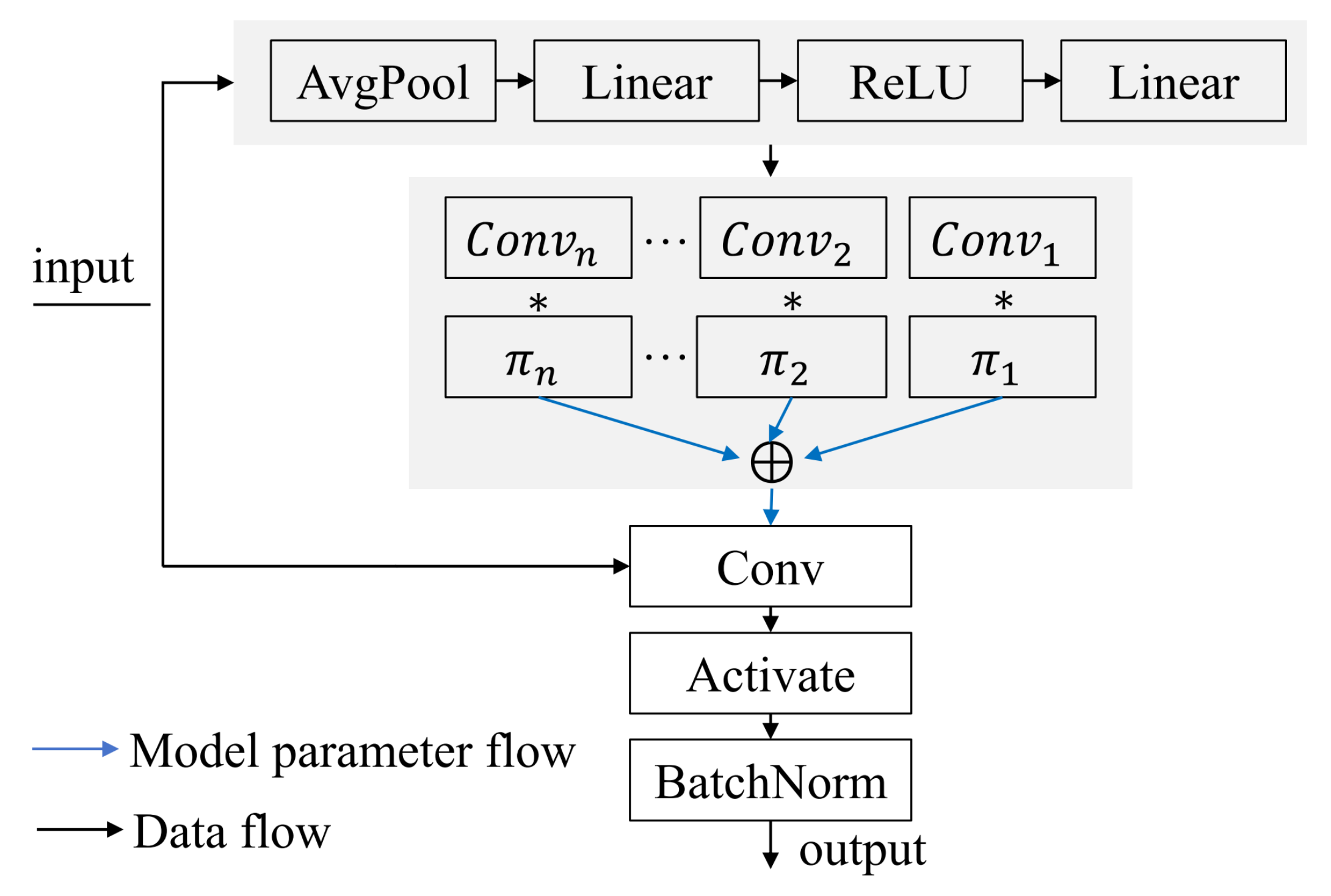
The dynamic convolution structure incorporates multiple variable convolutional kernels. These kernels, structurally similar to those in traditional CNNs, possess a unique ability: they dynamically adjust their parameters based on the characteristics of the input data. After each dynamic convolution unit, it is common to have a standard batch normalization (BatchNorm) layer and a non-linear activation function (such as ReLU). This maintains the advantages of the classic CNN design, and the structure is illustrated in Figure 2. Another significant advantage of dynamic convolution is its “plug-and-play” characteristic. This means that it can easily replace standard convolution operations in existing network models, whether they are 1 × 1, 1 × 3, or depthwise convolutions. Such flexibility not only allows dynamic convolution to be applicable to a variety of network architectures but also enhances the overall performance when processing datasets of different types and sizes.

Overall, dynamic convolution, with its dynamically adjustable kernels, offers a more effective and adaptable approach to handling complex datasets, which is challenging to achieve with traditional fixed-kernel architectures.

3. Methods

In this section, we first introduce the overall architecture of the model that we propose. We then delve into the structure and characteristics of our designed Multi-Branch Dynamic Convolution Network (MBDCNet), including a detailed explanation of its network architecture and an emphasis on how it integrates various components to enhance the diagnostic capabilities. Additionally, we provide a comprehensive discussion of a key element of MBDCNet—the dynamic convolution module. Finally, we describe the optimized loss function and its role.

3.1. Overview of the Proposed Model’s Architecture

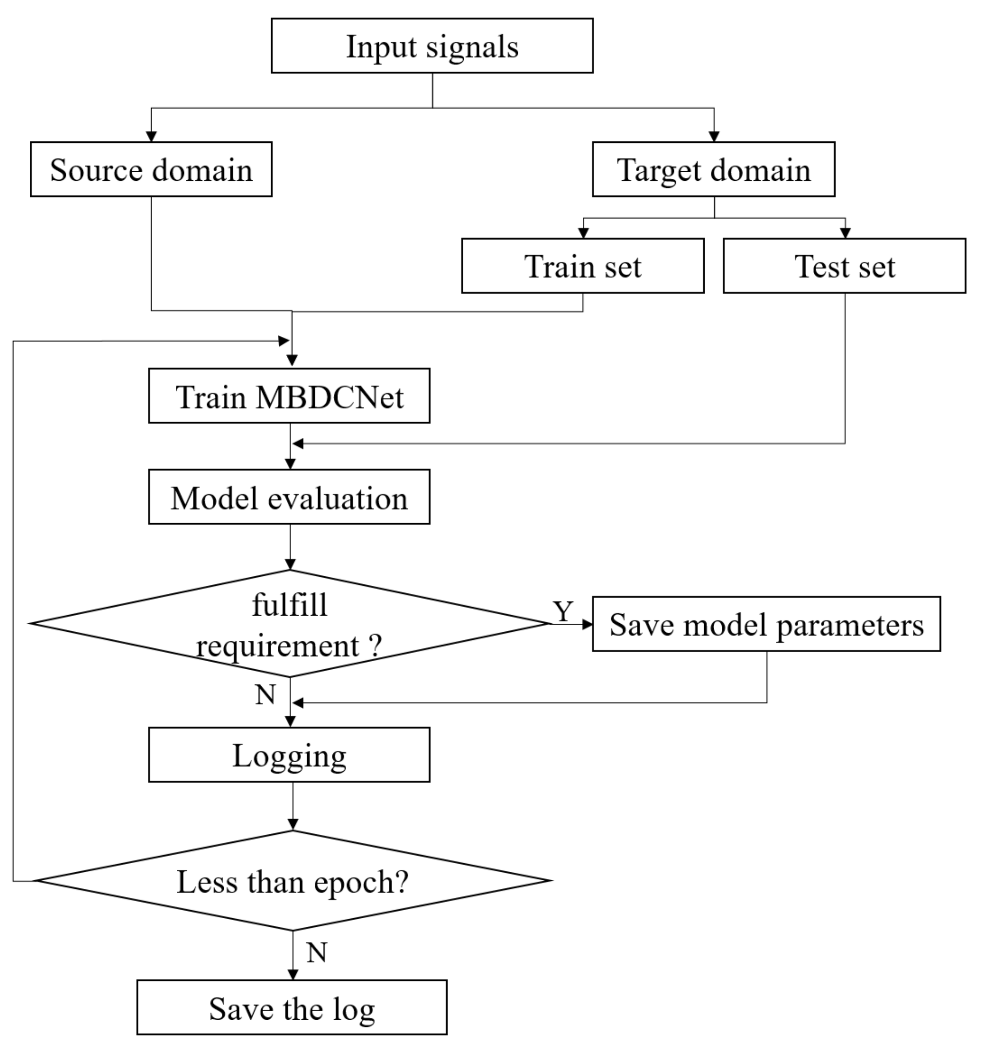
In practical bearing fault diagnosis applications, acquiring large-scale and comprehensively labeled datasets is often challenging. In this context, transfer learning emerges as an effective strategy, utilizing knowledge learned in the source domain (such as different types of bearings or datasets under various operating conditions) to significantly enhance the model performance in the target domain, even with limited data types. The primary advantage of this approach lies in enhancing the model’s generalization capability, reducing the training time and computational resource requirements, and improving the adaptability to new application scenarios. Accordingly, this paper proposes a bearing fault diagnosis method based on transfer learning. Its overall architecture encompasses four key components: data acquisition, model pre-training, transfer, and the visualization of the fault diagnosis results, as illustrated in Figure 3. Specifically, in the data acquisition phase, the method initially involves the preprocessing of raw data collected by sensors, identifying bearing fault vibration signals under different operating conditions, and dividing the dataset, while defining the scope of the source and target domain data. Subsequently, the designed MBDCNet is used for pre-training on these data, during which the model learns and saves key weight parameters, laying a solid foundation for the subsequent transfer phase, as depicted in Figure 4.

Subsequently, we migrate these parameters to the target domain and fine-tune them, as shown in Algorithm 1. Lastly, the fault diagnosis results are visualized for presentation.

Algorithm 1 Transfer Process

Input: configuration parameters: args, number of fault types: types Output: the health state of the bearing.   1: Load datasets and divide target domain dataset into training and validation sets.   2: Load the model: ${model}_f=MBDCnet\left(args\right);{model}_c=MBDCNet\left(args\right)$   3: Load pre-trained parameters saved from the model.   4: Define the optimizer and learning rate.   5: Define the loss function.   6: for epoch = 0 to epochs − 1 do   7:    for each batch in the dataset do   8:     Compute loss function for the source domain: $L_s=-\frac{1}{N}{\displaystyle \sum _{i=1}^N}{(1-p_i)}^{2}log\left(p_i\right)-{\displaystyle \sum _{i=1}^C}{y}_{i}log\left(\widehat{y_i}\right)$   9:     Compute loss function for the target domain: $L_t=-\frac{1}{N}{\displaystyle \sum _{i=1}^N}[{\left(y_i\right)}^{2}log\left(p(y_i=1)\right)+(1-y_i)log(1-p(y_i=1))]$ 10:     Perform backpropagation and update model parameters. 11:    end for 12:    Update learning rate if applicable. 13:    Validate the model using data from the target domain validation set. 14: end for

3.2. Feature Extraction Method Based on MBDCNet

In our research, we develop a novel multi-branch convolutional neural network architecture named MBDCNet, optimized specifically for the task of bearing fault feature extraction. The essence of this architecture lies in its multi-branch parallel processing mechanism, where each branch independently captures and analyzes different levels of features in the data. This enables the network to comprehensively handle complex signals, enhancing its adaptability to the complexity and diversity of bearing fault signals. The core components of MBDCNet include the dynamic convolution–batch normalization–ReLU (DBR) block, which integrates a dynamic convolution layer to dynamically adjust weights according to the input signal’s characteristics. It includes a batch normalization layer to reduce internal covariate shift, speeding up training, and a ReLU activation function to introduce non-linearity, boosting the model’s ability to capture complex non-linear relationships. Additionally, the dynamic convolution–batch normalization (DB) block deepens the feature hierarchy with additional dynamic convolution and batch normalization steps, enhancing the model’s sensitivity to subtle signal differences. The linear batch normalization–ReLU (LBR) block applies linear transformations to strengthen feature learning, uses batch normalization to stabilize the learning process, and incorporates a ReLU activation function to further enhance feature abstraction. The linear batch normalization–Sigmoid (LBS) block combines a linear layer with batch normalization to fine-tune the feature weights and employs a Sigmoid activation function in the final decision layer to output the probability of fault presence. Pooling layers use max pooling and average pooling to downsample features, aiming to reduce the computational load while preserving key feature information. This ensures that the network maintains sensitivity to important features even after dimension reduction.

The structure of MBDCNet is illustrated in Figure 5, primarily comprising three branches. The top branch of the network includes two DBR blocks and a Maxpool layer, tasked with extracting primary features from the input data and emphasizing key features through downsampling. The middle branch starts with a DBR block, uses a DB block for smooth feature extraction, and adds the output of the DB block to the original input of the DBR block, forming a residual connection. This design allows the original features to bypass the processing of two layers and flow directly to the downstream components, helping to alleviate the vanishing gradient problem while preserving the initial feature information. The results are then divided into two pathways: one passes directly through a ReLU activation, followed by a DBR block and a DB block, and finally another ReLU activation, each step refining and strengthening the feature representation. The other pathway travels through a DB block, followed by an LBR block and an LBS block, and finally combines with the results of the first path through a weighted sum operation. Another ReLU activation ensures the integration and enhancement of non-linear features, generating the final output for this branch. This structure enables the middle branch to merge features from different processing stages, efficiently analyzing and representing complex signals through residual connections and subsequent feature combinations—vital for bearing fault detection. The bottom branch consists of a DBR block and a Maxpool layer, also focusing on the capture and downsampling of basic features.

After processing across the branches, features undergo averaging in an Avgpool layer to integrate a broad range of contextual information, followed by a ReLU activation for additional non-linearity. Then, a linear layer maps the high-dimensional features to the output space, preparing for the final output, which may signify the results of classification or regression tasks.

The primary advantage of this multi-branch structure lies in its ability to facilitate collaborative work among different branches. Each branch, while maintaining its unique characteristics, collectively enhances the overall feature extraction capability of the network, and MBDCNet provides robust support for the comprehensive analysis of bearing fault signals through its multi-branch structure and detailed feature learning strategy. Figure 5 clearly demonstrates the hierarchical structure of MBDCNet and the flow of information between its multiple branches. This visual representation not only aids in understanding the unique function of each branch but also shows how they work together to boost the overall performance of the network. In our experimental validation, we will comprehensively assess the performance of MBDCNet on bearing fault datasets, verifying its effectiveness and superiority in practical applications for fault diagnosis tasks.

A key feature of the dynamic convolution network proposed in this article is the dynamic generation of convolutional kernel weights through a specially designed fully connected neural network, referred to as $weigh{t}_{net}$, enabling adaptive convolution operations. In this neural network, the channel-wise mean of the input sequence is provided to $weigh{t}_{net}$, the design that aids in extracting the overall features of the input sequence. The $weigh{t}_{net}$ comprises two linear layers and an activation function, as shown in Equation (2). Through the learning of these two linear layers, the network is capable of capturing complex non-linear relationships in the input sequence. The introduction of an activation function contributes to incorporating non-linear factors, thereby enhancing the network’s expressive capacity. Ultimately, $weigh{t}_{net}$ outputs a weight matrix for dynamic convolution, the shape of which is determined by the quantity of output channels, input channels, and convolutional kernels.

$$\begin{array}{c}\hfill \begin{array}{c}\hfill weigh{t}_{net}=view(Linear\left(ReLU\left(Linear\left(mean\left(x\right)\right)\right)\right),batchsize,ou{t}_{channels},i{n}_{channels},kernelsize),\end{array}\end{array}$$

(2)

$$\begin{array}{c}\hfill \begin{array}{c}\hfill out=view(Conv1d(view\left(x\right),weigh{t}_{net}),batchsize,ou{t}_{channels}),\end{array}\end{array}$$

(3)

Among them, $mean\left(x\right)$ represents the average value of the input sequence x along the channel dimension; $Linear$ denotes a linear layer; $ReLU$ represents the activation function and $view$ refers to the tensor reshaping operation; $Batchsize$ indicates the batch size; $ou{t}_{channels}$ represents output channels; $i{n}_{channels}$ denotes input channels; and $Conv1d$ signifies a one-dimensional convolution operation.

During the forward propagation process, this dynamic convolution module performs a one-dimensional convolution operation on the input sequence using the dynamically generated weight matrix, thereby producing an output tensor, as illustrated in Equation (3). This design enables the model to dynamically modify the kernels’ weights based on the varying characteristics of the input sequence, thereby achieving high adaptability to spatiotemporal changes. By introducing this dynamic feature, the module possesses a more flexible receptive field, allowing it to more effectively grasp both local and global characteristics within inputs, thus exhibiting excellent performance in processing complex, dynamic data. This design endows the dynamic convolution module with robust performance across a variety of application scenarios.

3.3. Design and Implementation of Loss Function

During the model pre-training phase, our target loss function comprises two components: CORAL [34] and cross-entropy loss. The combined application of these two loss functions aims to enhance the model’s generalization performance across different domain data. CORAL loss is used to measure the feature distribution differences between the source and target domains, with its mathematical expression shown in Equation (4). Cross-entropy loss is a commonly used loss function for multi-class classification tasks. For the model’s predicted probability distribution P and actual categories Y, the mathematical expression of cross-entropy loss is as illustrated in Equation (5).

$$\begin{array}{c}\hfill \begin{array}{c}\hfill CORA{l}_{loss}(X_s,X_t)=\frac{1}{4D^2}\left|\right|C_s-C_t{\left|\right|}_F^2,\end{array}\end{array}$$

(4)

Here, $X_s$ and $X_t$ represent the feature representations of the source and target domains, respectively, while $C_s$ and $C_t$ are their covariance matrices. The notation $\left|\right|·{\left|\right|}_F$ denotes the Frobenius norm of the matrix.

$$\begin{array}{c}\hfill \begin{array}{c}\hfill CrossEntrop{y}_{loss}(P,Y)=-\sum _{i=1}^c{y}_{i}log\left(\widehat{y_i}\right),\end{array}\end{array}$$

(5)

Among them, $y_i$ represents the ith element of the true label, and $\widehat{y_i}$ denotes the probability of the ith category as predicted by the model.

$$\begin{array}{c}\hfill \begin{array}{c}\hfill Loss=CORA{l}_{loss}+CrossEntrop{y}_{loss}.\end{array}\end{array}$$

(6)

The integrated utilization of these two loss functions facilitates the model in learning shared feature representations across different domains and enhances its generalization performance, as illustrated in Equation (6).

In the transfer phase, we propose a novel loss function for the fine-tuning of the parameters, as shown in Equation (7).

$$\begin{array}{c}\hfill \begin{array}{c}\hfill L_s=-\frac{1}{N}\sum _{i=1}^N{(1-p_i)}^2\ast log\left(p_i\right)-\sum _{i=1}^N{y}_{i}log\left(p_i\right),\end{array}\end{array}$$

(7)

Among them, N represents the number of samples, i denotes the ith sample, $p_i$ is the model’s predicted probability for sample i, and $y_i$ is the actual label for i.

From Equation (7), it can be observed that we have modified the loss function based on cross-entropy by introducing new elements, thereby designing a more comprehensive and adaptive loss function. This enhancement aims to more effectively discern the differences between categories in multi-class classification problems. By adjusting the weights of each sample, the network pays more attention to samples that are difficult to classify, thereby enhancing the adaptability to category imbalance and complex scenarios. This integrated loss function not only effectively drives the model to learn specific category features but also improves the overall classification performance. Moreover, this improved loss function provides a more powerful tool to deal with complex and changing real-world application scenarios, further solidifying the model’s robustness and generalization performance. This improvement is an effective supplement to the traditional cross-entropy loss function, making the model more reliable and robust in facing diverse challenges.

4. Experimental Results and Analysis

In this section, we first provide a detailed description of the experimental setup and the datasets used. Next, to validate the effectiveness of the proposed method, we conduct verification and in-depth analysis using two datasets. Finally, experimental and comparative analyses of the method proposed in this article are presented.

4.1. Experimental Setup and Evaluation Metrics

The implementation of the model and its experimental validation are conducted on a high-performance computing system equipped with a GeForce RTX 2080Ti GPU, utilizing PyTorch 1.11. In the model pre-training phase, the batch size is set to 256, the learning rate is 10⁻³, the optimizer is Adam, and the window size is 128. The most significant difference in the new task phase is that the learning rate is reduced to 10⁻⁶ to finely adjust the model parameters to adapt to the new tasks.

In this study, accuracy is used to evaluate the performance of the model in bearing fault diagnosis. Accuracy measures the proportion of samples correctly classified by the model relative to all samples. Specifically, it can be computed utilizing the formula below:

$$\begin{array}{c}\hfill \begin{array}{c}\hfill accuracy=\frac{N_c}{N}\times 100\%,\end{array}\end{array}$$

(8)

Among them, $N_c$ represents the number of correctly classified samples, and N represents the total number of samples.

Moreover, we use two types of accuracy metrics: the accuracy for known classes and the accuracy for all classes, represented as $known\_acc$ and $all\_acc$, respectively. The $known\_acc$ measures the accuracy for the classes that are known. It is calculated by dividing the number of correctly classified samples in the known categories by the total number of samples in these categories, as shown in Formula (9). The $all\_acc$ measures the overall accuracy across all classes, including both known and unknown ones. It is calculated by dividing the total number of correctly classified samples (across all categories) by the total number of samples in all categories, as shown in Formula (10).

$$\begin{array}{c}\hfill \begin{array}{c}\hfill known\_acc=\frac{N_{kc}}{N_k}\times 100\%,\end{array}\end{array}$$

(9)

$$\begin{array}{c}\hfill \begin{array}{c}\hfill all\_acc=\frac{N_{ac}}{N}\times 100\%,\end{array}\end{array}$$

(10)

Among them, $N_{kc}$ represents the number of correctly classified samples in known classes. $N_k$ represents the total number of samples in known classes. $N_{ac}$ represents the number of samples that are correctly classified across all classes.

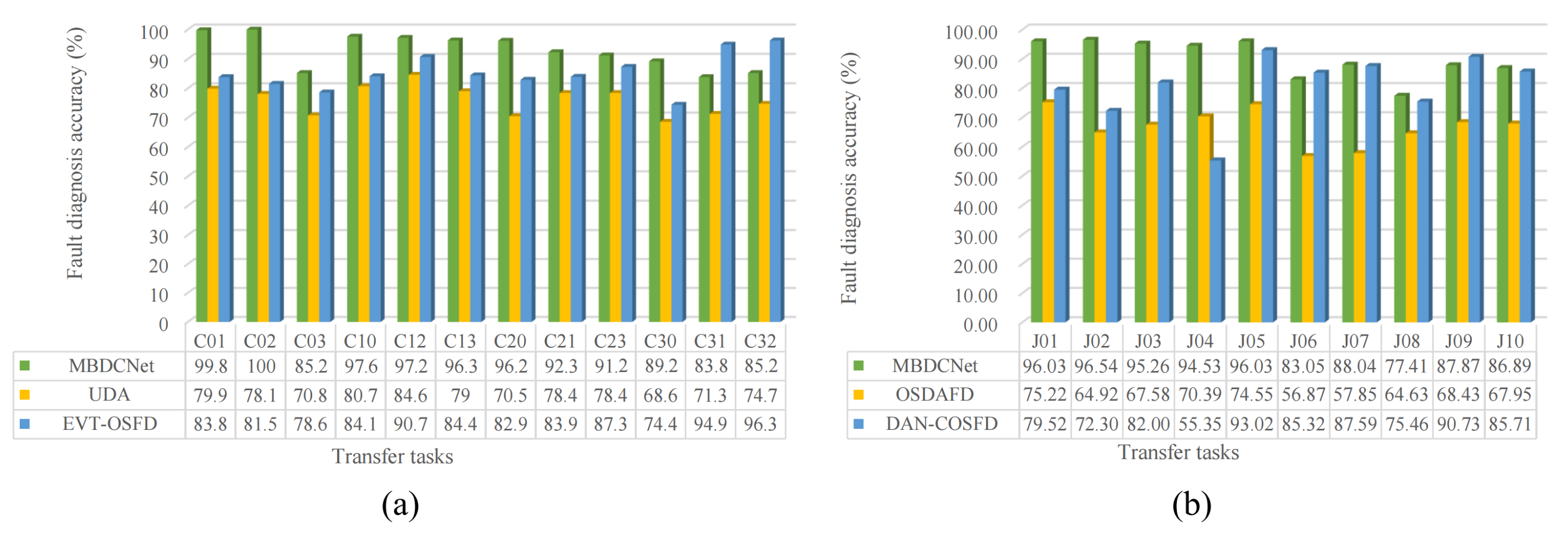
Additionally, in the comparative experiment for the CWRU dataset tasks, we utilize UDA (Universal Domain Adaptation) [35], EVT-OSFD (Open Set Fault Diagnosis by Extreme Value Theory) [26]. In the JUN dataset task, we compare the use of OSDAFD (Open-Set Domain Adaptation in Machinery Fault Diagnostics) [36], DAN-COSFD (Dual adversarial network for cross-domain open set fault diagnosis) [16], as it achieves higher accuracy in some tasks compared to the original results presented in the reference.

4.2. Dataset Description

1.

CWRU dataset

In our study, we first use the bearing dataset provided by Case Western Reserve University (CWRU) [37]. This dataset includes four bearing conditions, normal (N), inner race fault (IF), outer race fault (OF), and ball fault (BF), each with three different levels of damage (0.007, 0.014, 0.021 inches). The experimental data were obtained from a drive-end accelerometer under different load conditions: 0 hp, 1 hp, 2 hp, 3 hp, corresponding to 1797 rpm, 1772 rpm, 1750 rpm, 1730 rpm, respectively. All data were sampled at a frequency of 12 kHz. For this study, to assess the model’s performance in identifying and classifying various bearing faults, we selected 10 types of bearing conditions for analysis, as shown in

Table 1. CWRU dataset Information.

Label	Bearing Status	Fault Diameter (mil)
0	N	-
1	BF	7
2	BF	14
3	BF	21
4	IF	7
5	IF	14
6	IF	21
7	OF	7
8	OF	14
9	OF	21

.

2.

JNU dataset

The bearing dataset from Jiangnan University is specifically designed for research in bearing fault diagnosis and predictive maintenance [38]. It includes rolling bearing fault data obtained at various speeds, specifically encompassing the outer race, inner race, and rolling element fault types, as well as normal conditions. The dataset was collected at a sampling rate of 50 KHz and includes operating conditions at speeds of 600 rpm, 800 rpm, and 1000 rpm. The data are categorized into inner race fault (IF), outer race fault (OF), rolling element fault (BF), and normal (N) conditions, supporting a variety of fault diagnosis and machine learning research scenarios. For this study, data at speeds of 600 rpm and 1000 rpm were selected for model validation, with the bearing health conditions shown in

Table 2. JNU dataset information.

Label	Bearing Status
0	N
1	IF
2	OF
3	BF

.

To validate the effectiveness of the method proposed in this paper, this study utilizes two types of datasets, CWRU and JNU, to create various tasks. Initially, vibration signals are segmented using data overlap sampling techniques, with each sample containing 1024 data points. This approach aims to increase the sample size and enhance the robustness of the model. Further, to assess the model’s capability to classify different unknown fault types, as well as its adaptability to variations in category numbers between source and target tasks, we select multiple sample sets under different working conditions for the grouping of source and target tasks. The specific details of each task in the CWRU and JNU datasets are displayed in

Table 3. Task information of the datasets.

Dataset	Task	Source→ Target (Motor Load) (hp)	Source→ Target (Motor Speed) (rpm)	Source Label Set	Target Label Set
CWRU	C01	0→1	1797→1772	0, 1, 2, 3, 4, 5, 6	0, 1, 2, 3, 4, 7, 8, 9
	C02	0→2	1797→1750	0, 1, 2, 3, 4, 5, 6	0, 1, 2, 3, 4, 7, 8, 9
	C03	0→3	1797→1730	0, 1, 2, 3, 4, 5	0, 1, 2, 3, 4, 7, 8
	C10	1→0	1772→1797	0, 1, 2, 3, 4, 5	0, 1, 2, 3, 4, 7, 8
	C12	1→2	1772→1750	0, 1, 2, 3, 4, 5	0, 1, 6, 7
	C13	1→3	1772→1730	0, 1, 2, 3, 4, 5	0, 1, 6, 7
	C20	2→0	1750→1797	0, 1, 3, 5, 7, 9	0, 1, 2, 3, 4, 5
	C21	2→1	1750→1772	0, 1, 3, 5, 7, 9	0, 1, 2, 3, 4, 5
	C23	2→3	1750→1730	0, 1, 3, 5, 7	0, 1, 2, 3, 4
	C30	3→0	1730→1797	0, 1, 3, 5, 7	0, 1, 2, 3, 4
	C31	3→1	1730→1772	0, 2, 4, 6, 8	0, 2, 5
	C32	3→2	1730→1750	0, 2, 4, 6, 8	0, 2, 5
JNU	J01	-	600→1000	0, 1, 2, 3	0, 1, 2, 3
	J02			0, 1, 2
	J03			0, 1, 3
	J04			0, 1
	J05			0, 2
	J06		1000→600	0, 1, 2
	J07			0, 2, 3
	J08			0, 1
	J09			0, 2
	J10			0, 3

.

4.3. Experimental Results and Comparative Analysis

Our approach is evaluated on two standard datasets, CWRU and JNU, and compared to current advanced diagnostic methods. The comparative results are shown in

Table 4. The classification accuracy (%) of CWRU dataset.

Task	MBDCNet			UDA			EVT-OSFD
	all_acc	known_acc		all_acc	known_acc		all_acc	known_acc
C01	99.8	99.8		79.9	93.3		83.8	94.4
C02	100.0	100.0		78.1	89.1		81.5	93.7
C03	85.2	80.9		70.8	80.8		78.6	85.7
C10	97.6	96.4		80.7	89.4		84.1	90.2
C12	97.2	96.3		84.6	96.5		90.7	98.9
C13	96.3	95.1		79.0	93.3		84.4	94.2
C20	96.2	96.2		70.5	76.3		82.9	82.3
C21	92.3	96.2		78.4	83.1		83.9	87.0
C23	91.2	91.2		78.4	80.0		87.3	89.8
C30	89.2	89.2		68.6	73.4		74.4	73.7
C31	83.8	83.8		71.3	75.9		94.9	94.3
C32	85.2	85.2		74.7	79.9		96.3	96.2
Average	92.8	92.2		77.3	86.3		85.2	85.2

and

Table 5. The classification accuracy (%) of JNU dataset.

Task	MBDCNet			OSDAFD			DAN-COSFD
	all_acc	known_acc		all_acc	known_acc		all_acc	known_acc
J01	96.03	98.25		75.22	75.22		79.52	79.52
J02	96.54	98.12		64.92	65.40		72.30	70.01
J03	95.26	98.80		67.58	63.02		82.00	76.68
J04	94.53	97.75		70.39	70.04		55.35	72.46
J05	96.03	98.70		74.55	78.17		93.02	95.13
J06	83.05	85.01		56.87	60.36		85.32	83.24
J07	88.04	91.62		57.85	64.23		87.59	91.55
J08	77.41	77.23		64.63	64.92		75.46	67.14
J09	87.87	91.54		68.43	83.68		90.73	97.08
J10	86.89	90.76		67.95	73.81		85.71	90.17
Average	90.17	92.78		66.84	69.89		80.70	82.30

. As indicated in Table 4 and Table 5, the proposed model achieves the highest $all\_acc$ and $known\_all$ in most diagnostic tasks. Notably, our model achieves average accuracy of 90% on both datasets, reaching an optimal level. This not only reflects the model’s excellent classification ability across various categories but also demonstrates its outstanding performance in overall tasks. To more intuitively observe the differences in $all\_acc$ among various models, we have graphically represented these results. As illustrated in Figure 6, it is evident that the model that we propose has superior performance in terms of $all\_acc$ across most tasks.

In the analysis of the fault diagnosis results for the JNU dataset, it can be observed that our model demonstrates relatively low fluctuations in both $all\_acc$ and $known\_all$, indicating its high diagnostic stability. Even in instances where the accuracy is slightly below the optimal results, the model still exhibits robustness in handling diverse tasks and complex environments. For the tasks on the CWRU dataset, with the exception of C31 and C32, all results also indicate optimal performance. This further indicates that our model can reach high accuracy in the majority of tasks.

These encouraging experimental results demonstrate that our fault diagnosis method has advantages in accurately identifying unknown categories. By validating the model’s performance across different tasks, the study confirms its generalizability and adaptability, providing robust support for future research and practical applications in the field of fault diagnosis.

The analysis further illustrates that the MBDCNet model proposed in this article adopts key strategies in its design, showcasing exceptional capability in bearing fault diagnosis. The model’s use of dynamic convolution, batch normalization, activation functions, average pooling, and max pooling has been proven to enable the better capture of fault characteristics in bearing vibration signals. These components effectively enhance the model’s receptive field and spatiotemporal adaptability.

The experimental results effectively validate the crucial role of the pre-training phase. During this stage, the model employs cross-entropy loss and CORAL (domain-adaptive loss) for meticulous parameter adjustment, successfully learning the generic vibration features in the source domain, laying a solid foundation for subsequent transfer learning. In the transfer learning phase, these pre-trained parameters are applied to the target domain, combined with an improved loss function and adjusted learning rate, further enhancing the model’s performance. Fine-tuning allows our network to undergo adjustments based on the target data, better adapting to new environments. Despite the limited volume of data in the target domain, it is sufficient to support the effective fine-tuning of the network without the necessity of training from scratch. This approach enables us to retain the general features learned by the pre-trained model while also optimizing the model for specific tasks. Furthermore, fine-tuning helps to balance the information from the source and target domains during the transfer learning process, thereby preventing overfitting to the source domain data or underperforming in the target domain. This balance is crucial for the success of transfer learning, ensuring efficient knowledge transfer to the target domain and enhancing model performance and adaptability in new scenarios.

Overall, the experimental results clearly demonstrate that our method, with its meticulously designed model structure, its efficient pre-training and transfer learning strategies, and a loss function that thoroughly considers both source and target domain information, exhibits exceptional generalization in bearing fault diagnosis tasks. This ensures the model’s reliability and accuracy when dealing with complex real-world application scenarios.

To further analyze our proposed approach, we construct confusion matrices to detail the classification performance for each task on the CWRU and JNU datasets, as illustrated in Figure 7 and Figure 8. Confusion matrices provide an intuitive reflection of the model’s classification effectiveness. By visualizing the number of true positives, false positives, true negatives, and false negatives for different categories, we can comprehensively assess the performance of the algorithm. Each row of the confusion matrix represents an actual category, while each column represents the category predicted by the model. The elements on the diagonal of the matrix indicate the probabilities of correct classification by the model, whereas the off-diagonal elements represent the probabilities of misclassification. For instance, in the C01 task of the CWRU dataset (with target domain categories 0, 1, 2, 3, 4, 7, 8, 9), the values ’nan’ for true labels 5 and 6 indicate the absence of these categories. If the true label is 1 and the predicted label is 3, a corresponding value of 0.01 signifies that there is a 1% probability of category 1 being misclassified as category 3.

Finally, we also employ the t-Distributed Stochastic Neighbor Embedding (t-SNE) algorithm to visualize the performance of our model on different tasks across two datasets, as illustrated in Figure 9 and Figure 10. t-SNE is a dimensionality reduction technique, which we use to map high-dimensional features into a two-dimensional space, allowing for a more intuitive observation of the similarities and differences between samples. Through t-SNE visualization, we are able to observe the clustering of data points in a low-dimensional space. Taking the J03 task on the JNU dataset as an example, it is evident that category 1 was mistakenly classified as category 0, and category 3 was prone to being misclassified as category 1 and category 2. These visualizations also clearly show whether the features learned by the model enable samples of the same category to cluster more closely together, and whether there are clear boundaries between different categories on the t-SNE plot. Therefore, these visualization results provide us with an intuitive understanding of the model’s performance and the effectiveness of its feature learning, further supporting our evaluation of the algorithm.

5. Conclusions

This study introduces an innovative multi-scale bearing fault diagnosis method based on transfer learning, aimed at resolving the challenge of identifying unknown fault types in industrial equipment, thereby enhancing the accuracy of fault diagnosis and the reliability of the equipment. The proposed approach involves constructing MBDCNet and incorporating dynamic convolution, which effectively captures crucial information from bearing vibration signals and adapts to spatiotemporal variations in the input data. Furthermore, the use of pre-training and transfer learning strategies not only enables the model to learn more general vibration features in the source domain but also balances the information between the source and target domains through an improved loss function and fine-tuning of the learning rate, significantly enhancing the model’s robustness and generalization capability. Experimental results on the bearing datasets from Case Western Reserve University and Jiangnan University demonstrate high diagnostic accuracy under various working conditions, achieving the highest average accuracies of 92.8% and 90.2%, respectively. The effectiveness of the method is further confirmed by the confusion matrix and t-SNE visualization results. Overall, this study not only makes breakthrough progress in the recognition of new fault types but also offers a new research direction and practical solution to address the challenges posed by limited source task data in identifying new fault types in target tasks, presenting broad prospects for practical application.

While this study has achieved success on specific datasets, it has been conducted with a focus on different working conditions and tasks within the same dataset, without exploring the potential for cross-domain applications. Therefore, future work will investigate how to adjust or optimize the MBDCNet network and transfer learning strategies to cater to the needs of various industrial sectors, thereby broadening its application scope in industrial equipment maintenance. Moreover, overfitting problems may occur during transfer learning, especially when there are relatively few data in the target domain. We will continue to explore how to overcome these limitations through various strategies in future work.