An IoT Transfer Learning-Based Service for the Health Status Monitoring of Grapevines

Abstract

Grapevine is a valuable and profitable crop that is susceptible to various diseases, making effective disease detection crucial for crop monitoring. This work explores the use of deep learning-based plant disease detection as an alternative to traditional methods, employing an Internet of Things approach. An edge device, a Raspberry Pi 4 equipped with an RGB camera, is utilized to detect diseases in grapevine plants. Two lightweight deep learning models, MobileNet V2 and EfficientNet B0, were trained using a transfer learning technique on commercially available online dataset, then deployed and validated on field-site in an organic winery. The models’ performance was further enhanced using semantic segmentation with the Mobile-UNet algorithm. Results were reported through a web service using FastAPI. Both models achieved high training accuracies exceeding 95%, with MobileNet V2 slightly outperforming EfficientNet B0. During validation, MobileNet V2 achieved an accuracy of 94%, compared to 92% for EfficientNet B0. In terms of IoT deployment, MobileNet V2 exhibits faster inference time (330 ms) compared to EfficientNet B0 (390 ms), making it the preferred model for online deployment.

1. Introduction

The agricultural sector is of high importance to the worldwide economy as the rising global population creates a constantly increasing demand for food [1]. Plant diseases present a serious threat to the global agriculture industry, causing significant production losses and deterioration of the quality of the final product quality [2]. The emergence of diseases that affect plants has been more likely during the last decades due to the rapid increase in international produce exchanges and the general climate change (like global warming) [3,4,5,6,7]. The transmission of most emerging diseases is mainly due to biological invasions by plant pathogens, such as viruses, fungi, and bacteria [8,9]. Grapevine (Vitis vinifera subsp. Sativa L.) is a crop that is especially threatened by this kind of disease transmission throughout Europe [10].

Grapevine is an economically important plant that is cultivated mainly in the Northern hemisphere for grapes, either for consumption or for fermentation to produce wine. Its cultivation is hindered by a number of diseases worldwide, most important Powdery Mildew (induced by Uncinulanecator (Schw.) Burr.), Downy Mildew (induced by Plasmoparaviticola), Esca (induced by Phaeomoniella clamidospora and Phaeoacremonium aleophilum), Black rot (induced by Guignardia bidwellii), and Botrytis (induced by Botrytis Cinerea) [11]. These diseases can affect the plant leaves or the trunk, or they can directly affect the grapes. They have the potential to cause significant damage, resulting in huge yield losses or severely inferior product quality [12].

Traditional methods to determine the pathogen infecting the grapevine rely on visual inspection by trained experts and, for some pathogens, further evaluation by laboratory techniques may be necessary. The aforementioned techniques are destructive, time consuming, and, in the case of the visual inspection, may not always be accurate [13]. Moreover, infections are commonly addressed with the use of chemical compounds for preventive reasons or curable cases, or with destruction of crops to avoid further spread. This method, however, results in significant losses in crop yield, decrease in farmer’s income, and ecological contamination [14,15,16], without ensuring fewer losses [17].

In recent years, phytopathology and crop protection have been enhanced with the use of technologies such as robotics, sensing technologies, and artificial intelligence. These novel agro-technology methods belong to the field of precision agriculture (PA) and have helped minimise agricultural waste and maximise productivity [18,19,20,21]. To detect grapevine diseases, several studies have employed spectral sensing techniques, such as remote sensing that uses a multispectral camera on unmanned aerial vehicles (UAVs) [22,23], proximal sensing using thermal imaging [24,25] or hyperspectral sensing [26,27,28]. Although the use of the aforementioned equipment gives accurate results even at a pre-symptomatic level, they must be used by experienced scientific personnel, and they are also expensive.

For this reason, and with the rise of deep learning (DL), the use of simpler input signals, such as RGB images, has drawn scientific attention to disease detection [29,30]. Deep learning is a subcategory of machine learning and, as the name suggests, it is a method that employs a neural network with a large number of layers [31]. Thanks to convolutional neural networks (CNNs), DL has gained popularity in the field of computer vision, especially for classification problems [32,33,34], and has become a popular approach for plant disease identification [35,36,37,38]. Specifically for the detection of grapevine diseases, DL has been used to detect downy mildew and spider mite; this has been completed using RGB photos in Gutiérrez et al. (2021) [39] or esca in Alessandrini et al. (2021) [40].

Transfer learning (TL) is a DL approach that combats problems of limited data by training a pre-trained model that has proven its efficiency in classification problem using pre-existing datasets, such as those from online libraries [41]. In TL, the weights of those pre-trained models are kept and subsequently applied and partially updated to the new data [41]. Then, the knowledge of the original DL model is transferred to a new but similar classification problem, even though it does not have the same feature space or distribution [42]. The TL technique has been effectively used in the agricultural domain for disease detection in grapevines [43], tomatoes [44], wheat [45], and apple leaf [46]. After training, the models can be saved in a format that is readable by edge devices that can connect to a web services platform with the required sensors (cameras, complete with other sensors etc.) and be deployed for online validation, essentially giving farmers a way to precisely monitor the health status of their crops. This interconnection between the sensors in the field and the farmer’s computer or cell phone is called the Internet of Things (IoT) and has been successfully implemented in agriculture for smart irrigation [47,48], soil management [49,50], and pesticide management [51,52], among others [53]. IoT is, in other words, the internet-based interconnection of embedded computing devices, which allows them to send and receive data. The problem of crop’s health status monitoring is usually tackled by employing computer vision techniques with IoT [54], as in, for example, [55,56,57].

The this research aims to develop an integrated IoT system through validating the performance of an edge device, like the Raspberry Pi (RPi), based on DL algorithms, for the online detection of five grapevines diseases, based on symptoms in the leaves, in field conditions. The validation of the integrated system was performed in the Chatzivariti winery vineyard, where only Esca was identified. The system’s results are geotagged using an onboard GPS sensor, then are reported through Amazon Web Services (AWS) cloud platform on a web-based service in order to provide an online disease alert.

2. Materials and Methods

2.1. Datasets

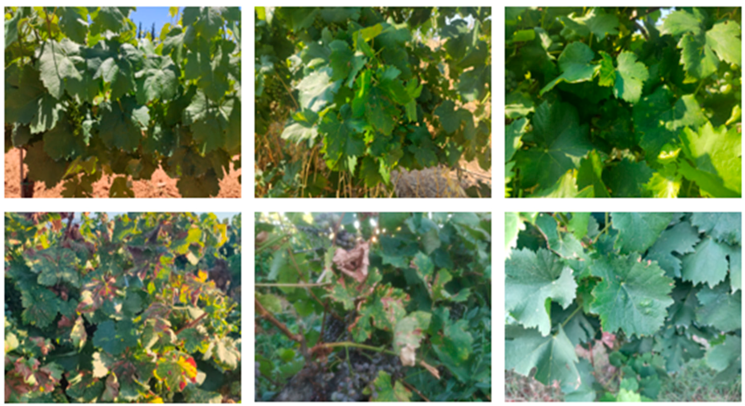
2.1.1. Training Data

The data utilised for training the Deep Learning models consisted of a comprehensive collection of images obtained from the Eden Library (EdenCore, Athens, Greece). The dataset encompasses diverse representations of both healthy plants and plants afflicted with various diseases, including fungal infections, viral diseases, and nutrient deficiencies. For the needs of this study, the dataset of grapevines was used (last version of data retrieved on December 2022). This dataset contains 1745 images depicting healthy grape leaves and leaves with diseases from five disease classes. A brief summary of the implemented training dataset is shown in

Table 1. The grapevine dataset classes by Eden Library with the number of images per class.

Dataset Class	Instances
Healthy	577
Esca	676
Powdery mildew	336
Downy mildew	96
Nitrogen deficiency	30
Eriophyes vitis	60

, and a sample set of random images from the Eden Library grapevines set is presented in Figure 1.

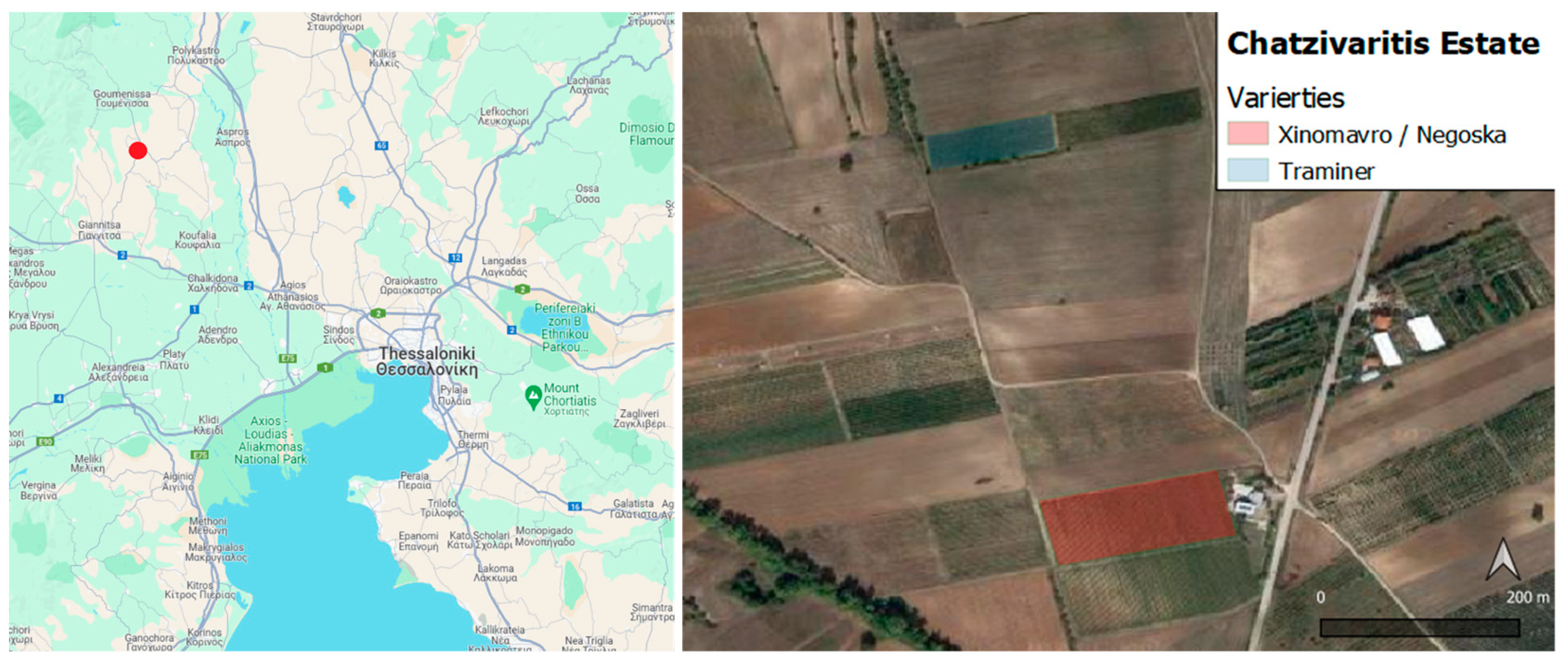
2.1.2. Validation Data

The validation of the models was performed in-field at the Chatzivarity winery in Goumenissa, Greece (Figure 2). The Chatzivarity Estate is an organic farm winery focused on the Greek varieties of Xinomavro, Negoska, Roditis, Malagousia, Muscat, and Assyrtico, while also cultivating the popular Sauvignon blanc, Merlot, Chardonnay, and Cabernet sauvignon in a smaller scale.

The three grape fields that the presented study focused on include the Xinomavro, Negoska, and Traminer varieties. These fields are visually presented in Figure 2, and they have grown on medium-textured sand and clay soils. Research was conducted in two fields of the winery. The first field (Field 1) is located adjacent to the estate’s main building, where 30 rows in the east side are cultivated with the Xinomavro variety and the 54 rows in the west are cultivated with the Negoska variety. The second field (Field 2) is located 500 m to the north of the estate’s main building and consists of the Traminer variety. The field survey for the validation of the developed models took place on 4 August 2022. During the survey, both fields had visible symptoms of Esca, although Field 1 was in a better condition than Field 2.

The visual examination of the disease’s symptoms by the expert phytopathologists served as the foundation for the health status evaluation of the Chatzivarity case plants. The spots selected to validate the models were spots in a row that had both healthy and infected plants. Esca fungus has very discrete symptoms and is easily recognizable by a trained expert. Specifically, an interveinal “striping” is the foliar sign of Esca. The “stripes”, which begin as yellow in white cultivars and crimson in red cultivars, dry out and turn necrotic.

2.2. Transfer Learning

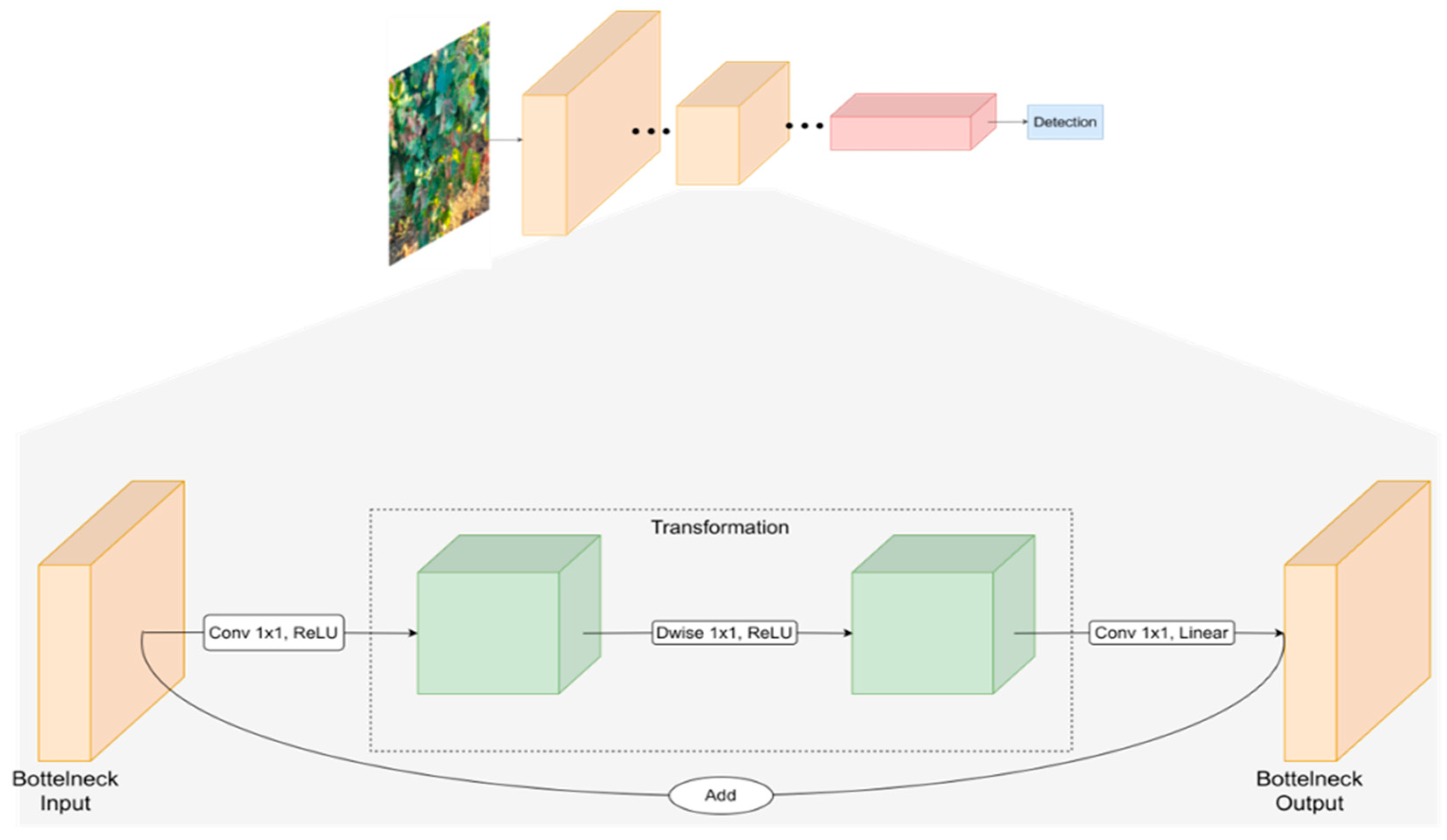
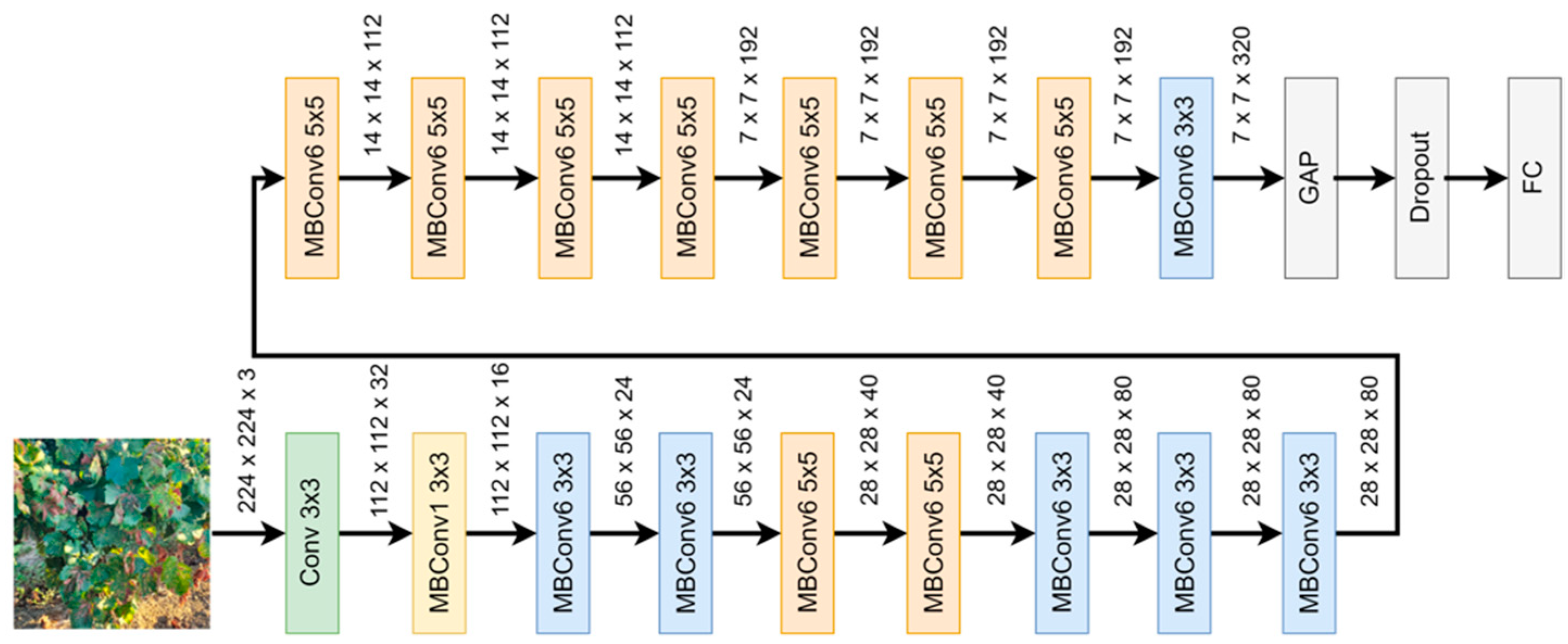
2.2.1. Deep Learning Models

The models’ training was based on pretrained models that have been shown to provide efficient performance and generalisation capabilities in various computer vision tasks [35]. The models that were chosen for this reason were the MobileNet v2 and the EfficientNet B0. These two models have been employed due to their potential capability to be computationally efficient and their structural differences in the feature extraction layer architecture.

MobileNetV1 was developed by taking inspiration from the conventional VGG architecture, which involves stacking convolutional layers to enhance accuracy [58]. Nonetheless, the issue of gradient vanishing arises when an excessive number of convolutional layers are stacked. To address this, ResNet introduced residual blocks that facilitate the smooth flow of information between layers, including feature reuse during forward propagation and alleviation of gradient vanishing during back propagation [59]. Consequently, MobileNetV2, introduced by Sandler et al., (2018) [60], is a CNN architecture that incorporates the depth separable convolution [61] from MobileNetV1 and adopts ResNet’s residual structure. MobileNetV2 introduces two key improvements: the utilisation of linear bottleneck, as is described in the architecture of Squeeznet, and inverted residual blocks within the network [62]. As illustrated in Figure 3, MobileNetV2’s fundamental building block is a depth separable convolution block based on inverted residuals with a linear bottleneck. As a whole, the architecture of MobileNetV2 contains the initial fully convolution layer with 32 filters, followed by 19 residual bottleneck layers.

EfficientNet B0, introduced by Tan and Le, 2019 [63], is a CNN that incorporates specialised convolutional blocks, known as Mobile Inverted Residual Bottleneck Convolution (MBConv) [60,63], with squeeze-and-excitation optimization [64] in its architecture. These MBconv blocks play a crucial role in capturing and processing features at various scales, enhancing the model’s performance and efficiency. Figure 4 shows the architecture of EfficientNet B0, where MBConv1 refers to a MBConv block with a 1 × 1 kernel size, enabling the capture of fine-grained details and facilitating information fusion across different channels. In contrast, MBConv6 represents an MBConv block with a larger 6 × 6 kernel size, focusing on capturing broader context and higher-level semantic information. The combination of MBConv1 and MBConv6 blocks in EfficientNet B0 enables the model to extract multi-scale features effectively, contributing to its impressive performance in diverse image recognition tasks. For this work, a Global Average Pooling and a Dropout layer were added to the last layers before the fully connected layer.

The procedures and the models outlined in this paper were implemented using the TensorFlow library (version 2.10) within a Python-based programming environment (Python version 3.9). The whole system was trained on a graphical processing unit (GPU) (GeForce RTX 3080, nVIDIA, Santa Clara, CA, USA) with compute unified device architecture (CUDA) enabled.

2.2.2. Training through Transfer Learning

These DL models have been trained on the ImageNet dataset, a benchmark dataset that consists of over one million images for training and validation purposes (almost 90% of the total data), along with a hundred thousand images for testing (almost 10% of the total data). In this study, a transfer learning (TL) approach was employed, utilising the inherited training weights from the models’ prior training on the ImageNet dataset. TL, by definition, is a deep learning technique that uses previously trained models as a foundation for new tasks. Instead of starting from zero when training a model, the information and features gleaned from a sizable dataset are used for a new, related task. This method saves time and resources because the pre-trained model is already well-versed in broad patterns and may be adjusted to excel at the given task. Even with the limited amount of data available for the new task, it enables faster training and better performance.

TL can involve changing either only part of the convolutional base or the whole base, depending on the specific requirements of the task. The approach where only a portion of the convolutional base is updated is called “Feature Extraction” as the pre-trained weights are used as a fixed feature extractor in a high layer level, while the lower layers are trained in the target task. Meanwhile, the approach where the weights of the whole convolutional base are updated is called “Fine Tuning”. In this approach, the weights of the base are adjusted along with the newly added layers in order to have a model that is more flexible model in terms of adaptation to the new task as it makes modifications to the learned representations at different levels of abstraction.

In this study, a fine-tuning approach was considered, and thus, the training process involved keeping the models’ convolutional architecture intact and updating the model weights in all the base layers. The weights were updated, using the grapevines subset data taken by the Eden Library dataset.

Specifically, the base models were instantiated, having all of the base layers’ weights unfrozen, and the fully connected (FC) layer with the 1000 classes from the ImageNet with a dense layer was replaced with six outputs, where each output corresponded to the probability of the identified health status label on the grapevine. The grapevines subset from the Eden Library dataset was used for the initial training of the models and for updating the weights. The validation of the model was performed online on the vineyard of the Chatzivarity winery after having deployed the model on a Raspberry Pi 4 (RPi) platform, with a custom RGB camera module mounted on it.

2.2.3. Data Preprocessing and Hyperparameter Tuning

Prior to their integration to the DL models, the data are subjected to preprocessing techniques. The first step is resizing the images into a specific range for each of the selected. MobileNet v2 and EfficientNet b0 have an expected input size of 224 × 224 pixels. Specifically, MobileNet may have input images with a higher size than 32 × 32, and higher resolutions lead to slower but better model performance. TensorFlow, the python library chosen for the implementation of the DL models in this study, requires an image input of 224 × 224, so image preprocessing focused on this size would be appropriate for all the study cases of this research. Additionally, a normalisation to the range of [0, 1] is performed by dividing the pixel values by 255.

Due to the fact that the classes of the grapevine subset of the Eden Library dataset is very imbalanced (Table 1), data augmentation on the training set was performed. Healthy and esca classes were reduced to 550 images each, and various data augmentation techniques were employed for the rest of the classes, using random combinations and values of rotation, shearing, zooming, and flipping of the images, as described in

Table 2. Data augmentation parameters and selected values.

Data Augmentation Parameter	Possible Values
Rotation	[−30°, 30°, 5°] *
Image Shearing	-
Image Zooming	0.8, 0.9, 1.1, 1.2
Image Flipping	Horizontally, vertically

* can take any integral value in the specified range, with a step of +5°.

, until each class consisted of a representative number of images close to 550.

The selection of the appropriate hyperparameters for model training is a critical topic that is addressed in this work. Hyperparameters may have a significant impact on how well the DL model works. In order to determine the best strategy that can be applied to the examined DL models, different methods can be selected, between including grid search, random search, and Bayesian optimization. In this work, the grid search method was employed and the hyperparameter values that were tested are shown in

Table 3. Tested values of the different deep learning hyperparameters for their tuning using the grid search method.

Hyperparameter	Possible Values
Epoch number	10, 20, 30, 50
Optimization algorithm	RMSprop, Adam, SGD
Learning rate	0.1, 5 × 10−2, 10−2, 10−3, 10−4
Batch size	16, 32, 64
Dropout rate	0.1, 0.2, 0.3

. The selection values were guided by a combination of empirical experience of the authors and insights drawn from relevant literature. While the specific values were chosen randomly to ensure a broad and unbiased exploration of the parameter space, they were informed by commonly used ranges and best practices as are documented in existing studies.

In the output of the base models, the global average pooling technique was applied in order to prevent overfitting and improve the generalisation performance. Finally, the SoftMax activation function was used on the output layer and the ReLU activation function in the rest of the FC layer.

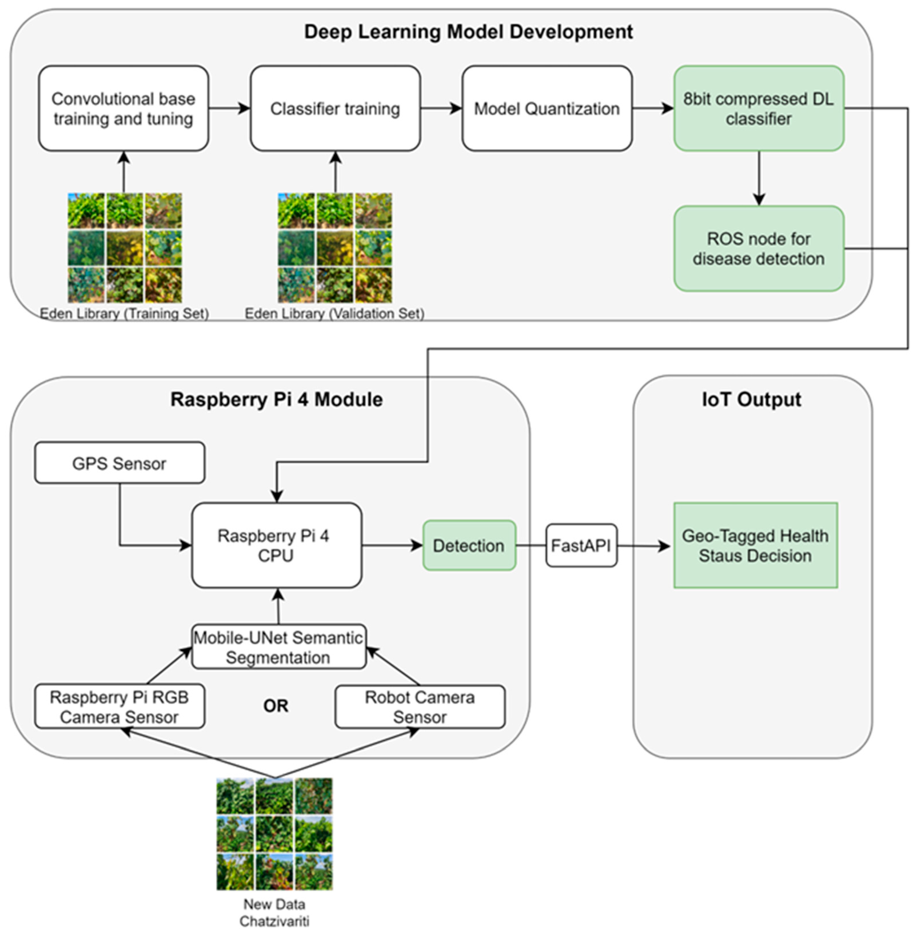
2.3. Model Integration to the Raspberry Pi 4 for Online Disease Assessment

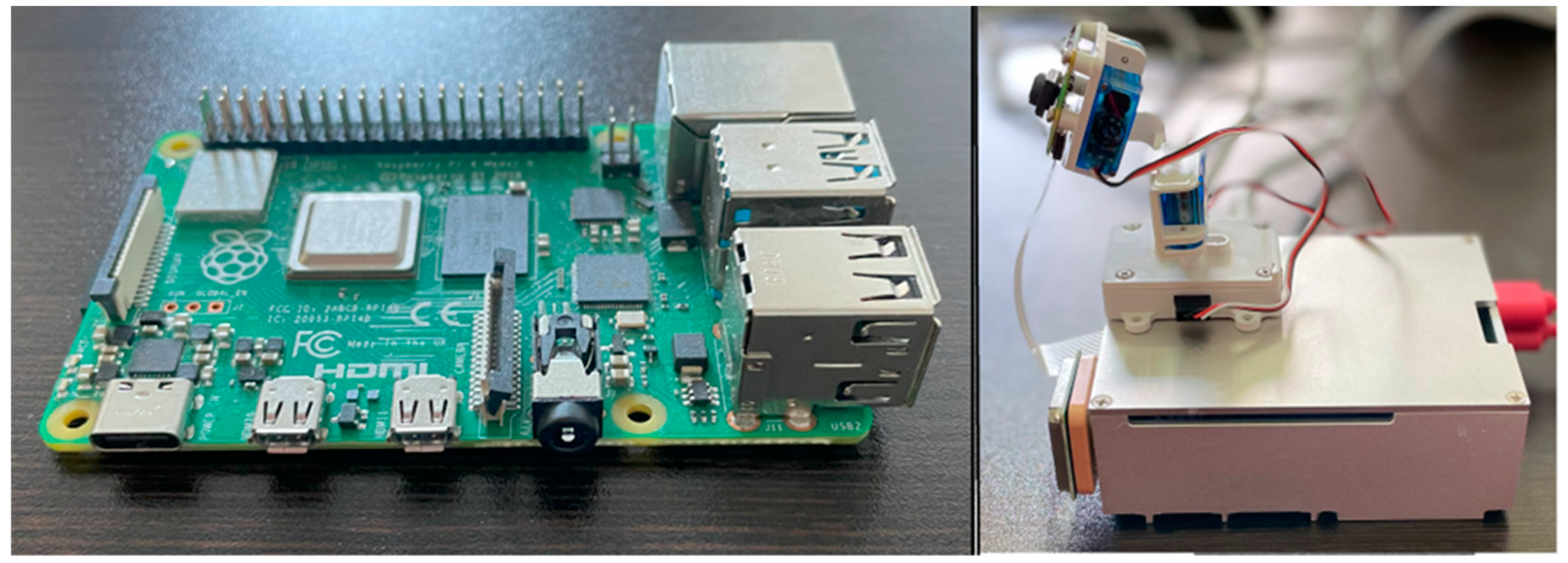
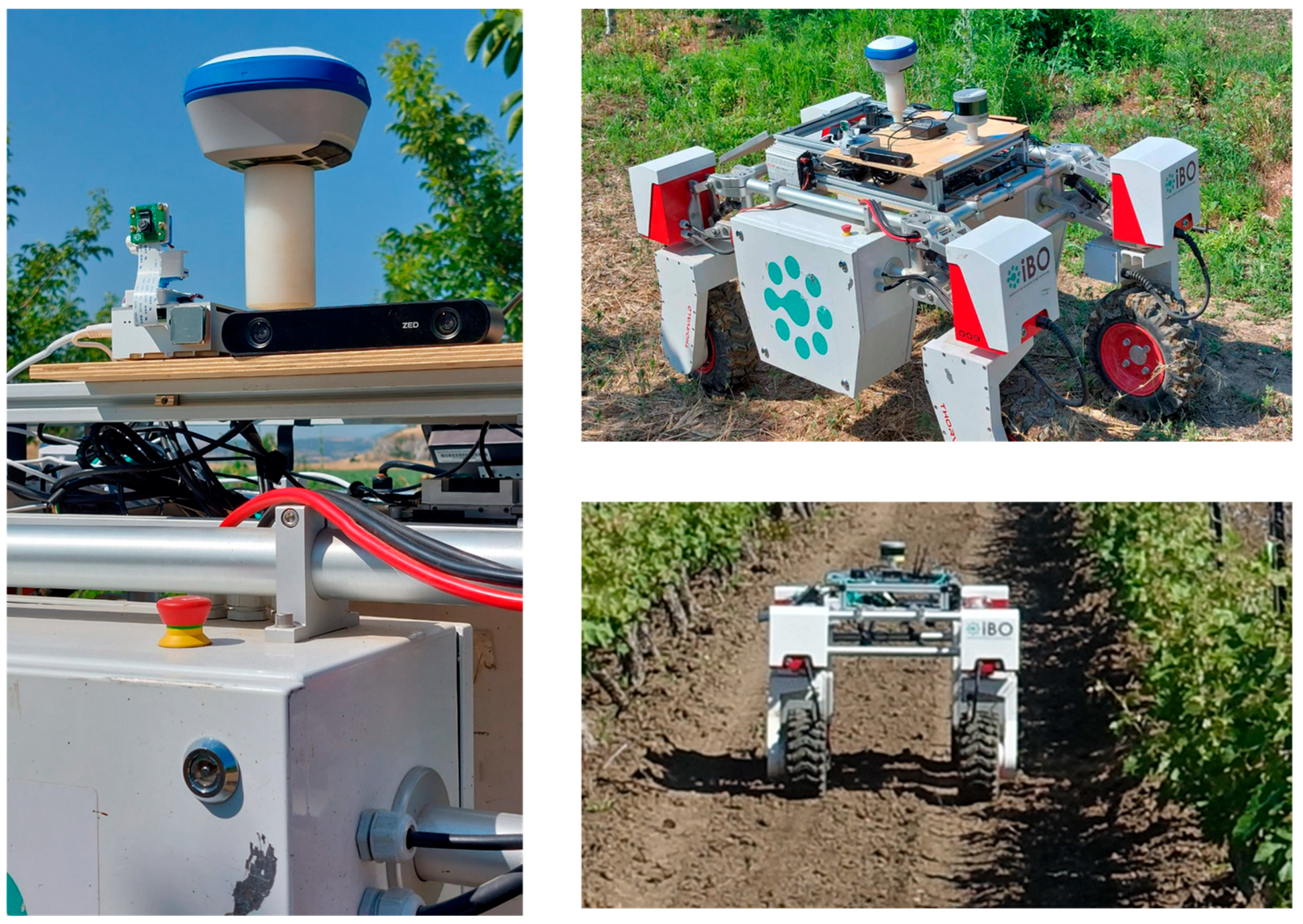
2.3.1. Hardware

For the current research, a Raspberry Pi 4 (RPi) model B was used (Figure 5) that has a quad-core ARM Cortex-BCM2711 CPU of 15 GHz and 8 GB of RAM. Additionally, there are 40 GPIO pins, a full HDMI port, 4 USB ports, an ethernet port, a 3.5 mm audio jack, a video camera interface (CSI), the display interface (DSI), and a micro SD card slot. The RPi is connected with a U-Blox Neo-6M GPS Module to record the coordinates for each capture. Finally, RPi was connected to an 8 MP Raspberry Pi Camera Module 2 (RB-CAMERAV2) via a flex cable (Figure 5). RPi was chosen for model integration as it has a relatively higher computational power compared to other microcontrollers, like Arduino or STM32 controllers, and it has a powerful CPU and a GPU that can be leveraged for certain types of parallel computations. Additionally, it can run a full-fledged Linux OS, providing access to a wide range of software libraries and tools, like TensorFlow. Finally, it provides higher built-in networking capabilities, making it ideal for IoT projects that require network communication.

A robust steel case was used for the protection of the RPi, ensuring the safety of the device under harsh conditions, such as exposure to sunlight and occasional raindrops. The total cost of the proposed system with all components was approximately EUR 160.

2.3.2. Model Integration

After the training process, the trained models with the highest validation accuracy (the accuracy of the model in the end of the validation phase, before the model deployment) on the disease identification on the field conditions from both MobileNet V2 and EfficientNet B0 were chosen to be used for the online deployment. Prior to the integration of the models with the RPi, they need to be converted to a format that can be easily deployable [65,66,67]. The saved models were subjected to post-training quantization. This technique involves converting a pretrained TensorFlow model into a TensorFlow Lite format using the TensorFlow Lite Converter, enabling quantization of the model’s parameters. By applying this approach, the model size is reduced and CPU and hardware acceleration latency are improved while maintaining satisfactory levels of classification accuracy [68]. This quantization technique better balances the trade-off of model size reduction and potential accuracy degradation as the complexity and the architecture of the deep learning models can influence the effectiveness and compatibility of the different approaches. Additionally, other factors that should be considered are the hardware constraints and requirements. For these reasons, the full integer quantization approach was considered as it is supported by microcontrollers such as the RPi, providing a 4-fold model compression and maintaining most of the models’ predictive ability.

After generating the quantized model, it was imported into the RPi, which was equipped with a camera and a GPS module. Two image acquisition approaches were considered for RPi integration. The first approach involved using the RPi as a standalone handheld device, acquiring images directly from the mounted RGB camera module. The second approach involved incorporating the RPi onto an unmanned ground vehicle (UGV) and making use of its own camera sensors. For this reason, a Robot Operating System (ROS) node was developed to subscribe to an external camera’s specified topic on the UGV platform and publish the results. In both cases, the imported images from the camera underwent the same image compression techniques applied during model training, including compression to a size of 224 × 224 pixels and image normalisation within the range of [0, 1]. The output of the RPi model consisted of string-type messages containing the predicted class for each captured image and the corresponding GPS coordinates.

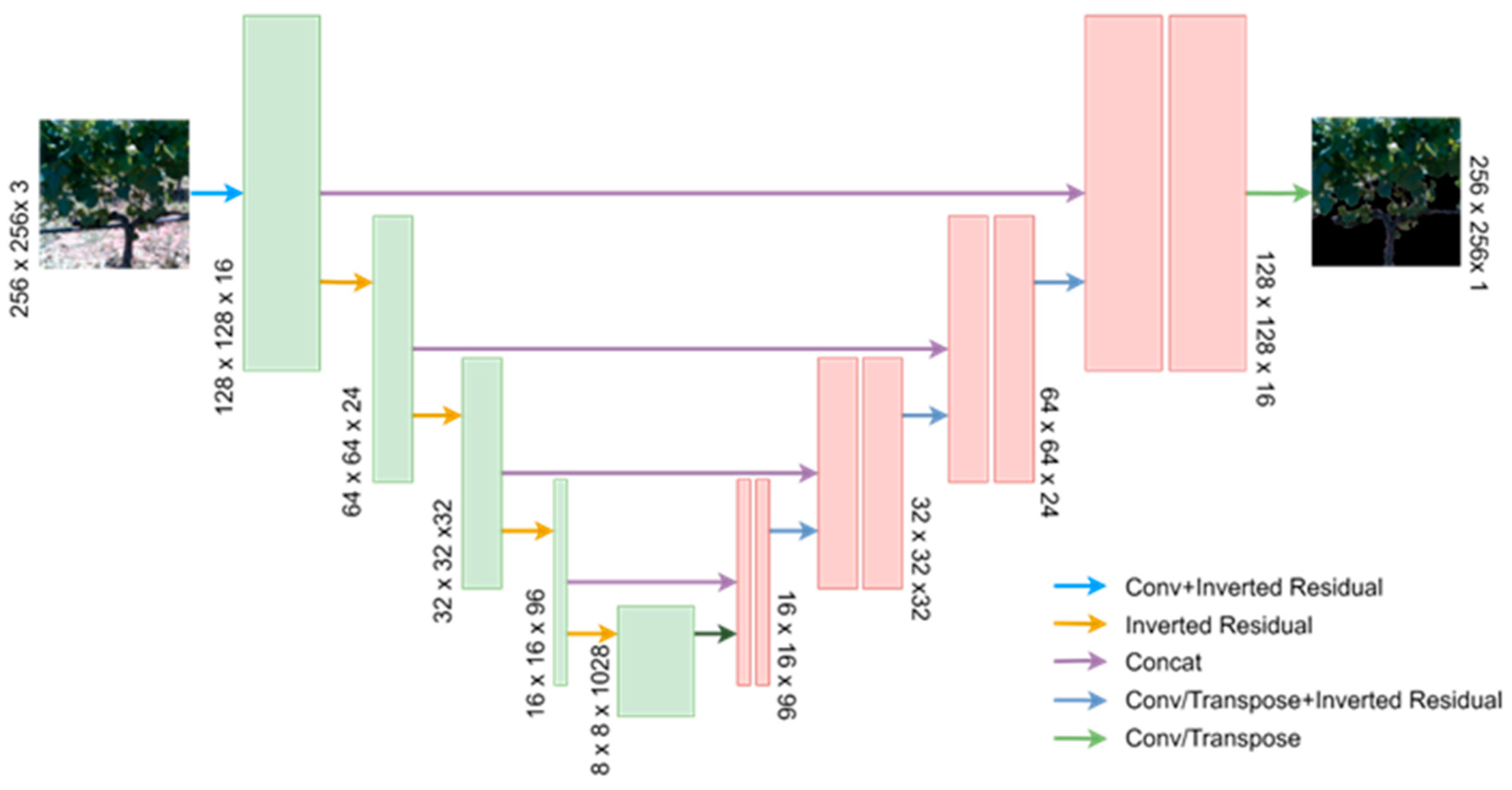
2.3.3. Semantic Segmentation Using Mobile-UNet

Eden Library’s data include photos of grapevine plants with little or no background noise. During the online survey at the Chatzivariti winery, there were instances where the pictures had significant background information from the soil or the grapevine row behind the one of the measurements. Thus, in order to reduce the background noise from the raw incoming video stream and increase the chances of a successful implementation of the deep learning models, a semantic segmentation algorithm was also developed. Mobile-UNet was chosen as the algorithm that would perform the task in this paper.

U-Net, proposed by Ronneberger et al. (2015), is a semantic segmentation convolutional network that exhibits a symmetric distribution, utilising shallow high-resolution feature maps to address pixel localization and deep low-resolution feature maps to handle pixel classification [69]. The network incorporates skip connections, allowing for the preservation of both location and feature information, making it suitable for pixel-level semantic segmentation tasks. The architecture follows a U-shaped encoding and decoding structure (Figure 6), leveraging the VGG network (Simonyan and Zisserman) in the encoding stage and using up-sampling modules in the decoding stage.

Despite the attention that the U-Net had gained, especially in medical applications, due to the excellent performance in the segmentation task, it exhibits adaptability in small datasets in particular due to its low number of weight parameters [70]. Additionally, due to its VGG approach in the encoding stage, its detection approach is very time consuming. For this reason, Jing et al. (2022) proposed replacing the encoding part of the original U-Net with MobileNet’s depthwise separable convolutions [71]. By leveraging these building blocks in the encoding stage and skip connections, Mobile-UNet reduces the number of parameters and operations (almost 3% of the respective VGG network), enabling faster inference and better resource utilisation on mobile devices.

The architecture is summarised in Figure 6, from which it can be seen that the feature extraction layers of the pre-trained MobileNetV2 are employed to replace the down-sampling stage of the original U-Net. As for the up-sampling part, it consists of five deconvolution layers and four inverted residual blocks. This configuration ensures that the input and output dimensions of Mobile-Unet remain consistent.

U-Net has proven its value in semantic segmentation tasks in the field of agriculture as it can successfully segment images with a high level of details, such as navigation paths [72] and weed detection [73]. Likewise, Mobile-UNet has proven that it has comparable results with the original U-Net, and thus is expected to have a satisfactory segmentation performance in this study [71]. The loss function that was used for the training was the categorical cross entropy. Given its efficacy in the task of semantic segmentation, it is worth noting that, in this paper, the Mobile-UNet algorithm was used solely as a tool to assist the validation results of the models, and for this reason, even though its performance is reported in the results section, it is of no further scientific interest.

2.3.4. Data Acquisition Layout

The data acquisition in the Chatzivariti winery was performed by mounting the proposed system on an UGV (Thorvald, SAGA Robotics SA, Oslo, Norway) at a fixed height of 88 cm and a vertical distance from the crop canopy in the range of 95 to 105 cm. Although the UGV was equipped with an RGB-D (ZED 2 depth by Stereolabs Inc., San Francisco, CA, USA) in this study, the RPi camera was used for the image capturing, looking vertically in the crops, and was placed in the left side of the UGV platform (Figure 7).

The UGV’s speed was kept constant at 1.25 m/s (±0.1 m/s). The video capturing frame rate was set to be as low as 3 fps. A low frame rate helps with the computational requirements needed for the online inference of the segmentation and the DL models. Additionally, a higher frame rate would give too much information from the same region of the crop, which is of no use for the model’s performance.

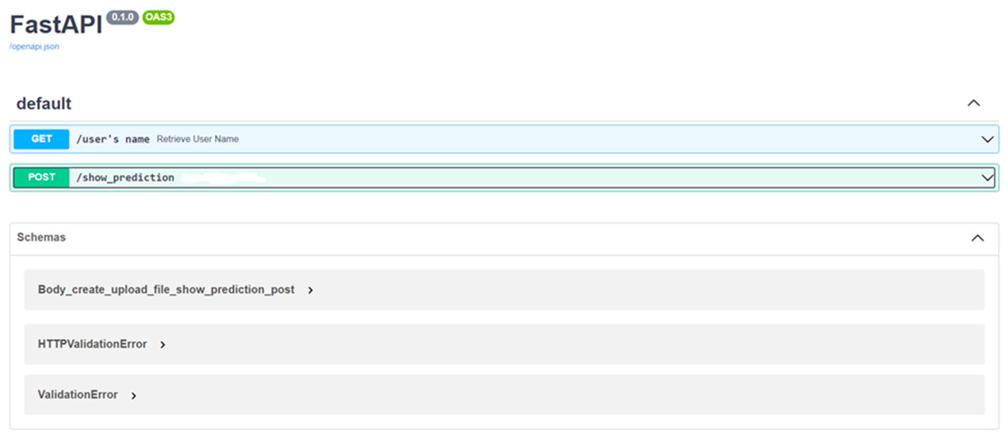
2.4. FastAPI Web Service Interface

The proposed study involves incorporating a transfer learning algorithm for disease detection into a web service architecture. The web service provides a user-friendly environment for disease detection by acting as an interface between end-users and the DL model. The architecture consists of multiple components, such as a client-side interface, a server-side application, and an API, built on FastAPI, to facilitate communication between the web service and the machine learning model. The API specifies a collection of endpoints that permit the transmission of data and requests between the client and the server. Through these endpoints, the web service can receive the prediction results of the TL model and provide a determination of the plants’ healthy or diseased status. In addition, the API enables the retrieval of model information, including performance metrics and training status, which can be displayed to the user via the web service interface.

The incorporation of the transfer learning algorithm for disease detection into the web service enables real-time disease detection on patient data. Through the web service interface, the decision of the TL algorithm can be easily accessed remotely and be interconnected to other agricultural web services that would use the signal of the detection of unhealthy plants as a trigger to enable procedures, such as spraying of appropriate pesticides.

To facilitate communication between ROS and FastAPI, a communication bridging component was developed to send the decision message published by the ROS node to the FastAPI web service using HTTP requests. A schematic representation of the whole IoT integration is given in Figure 8.

2.5. Model Evaluation Metrics

For the models’ evaluation, the accuracy and F1 score metrics were used. As shown in Equation (1), accuracy is the ratio of the correct predictions over the sum of all predictions (correct and wrong). In the following equation, TN, TP, FN, and FP represent the true negative, true positive, false negative, and false positive values in the models’ confusion matrix. F1 score, on the other hand (Equation (2)), is the harmonic mean of precision (TP over TP and FP) and recall (TP over TP and FN) and provides a balance between these two metrics.

$$Accuracy=\frac{TP+TN}{TP+TN+FP+FN}$$

(1)

$$F1 score=\frac{2(Precision·Recall)}{Precision+Recall}$$

(2)

Accuracy was decided as the evaluation metric for this paper as it is a widely used metric. Accuracy, though, assumes a somewhat balanced distribution of the training examples throughout the different classes in order to give a representative evaluation on the models’ performance. In this study, after the data augmentation that occurred, all six classes contained almost the same number of images (the deviation between the images of each class was, at maximum, 3%). The harmonic mean is used to compute the F1 score because it gives more weight to lower values. This means that, if either precision or recall is low, the F1 score will be significantly affected, encouraging a balance between the two metrics. This makes it robust in imbalanced class distribution. F1 score in this work is used in order to validate the accuracy results as both metrics are expected to have similar outcomes.

Furthermore, the evaluation of the overlap between predicted segmentations was performed using the Intersection over Union (IoU), also referred to as the Jaccard index. This was computed to measure the degree of intersection between the predicted and actual segmentations, as described in Equation (3).

$$IoU=\frac{TP}{TP+FN+FP}$$

(3)

3. Results

3.1. Hyperparameter Tuning

As was described, two DL models that were examined for their ability to detect diseases in grapevine plants. The training was performed using the data from the grapevine dataset of the Eden Library online dataset. The models that were considered were the MobileNet V2 and EfficientNet B0.

For this reason, the first thing that had to be determined was the selection of the most suitable hyperparameters for the optimal training of the models. The grid search method involves exhaustively searching the set of the hyperparameter values that were defined in Table 3 to determine the best combination that yields the highest performance in the models. The results have shown that the Adam optimization algorithm with 20 epochs and a batch size of 16 was chosen for both tested classifiers. The best dropout rate was found to be 0.2 for EfficientNet B0 and 0.1 for MobileNet V2 and, finally, the learning rate also varied for each model, with the most suitable value for EfficientNet B0 being 10⁻³, and for MobileNet V2, being 10⁻⁴.

Additionally, in order to further optimise the grid search methods and the overall performance of the training process, the implementation of certain callbacks was involved. Two key callbacks utilised were the early stopping and model checkpoint. The early stopping callback monitors the validation loss, allowing for early termination of the training if no improvement is observed over a defined number of epochs (defined as “patience”). The patience level was chosen to be four epochs in this study. The model checkpoint callback was utilised to save the weights of the model at the end of each epoch, keeping every time the epoch with the best validation accuracy, ensuring that the best performing model will be preserved for use in the deployment of the model.

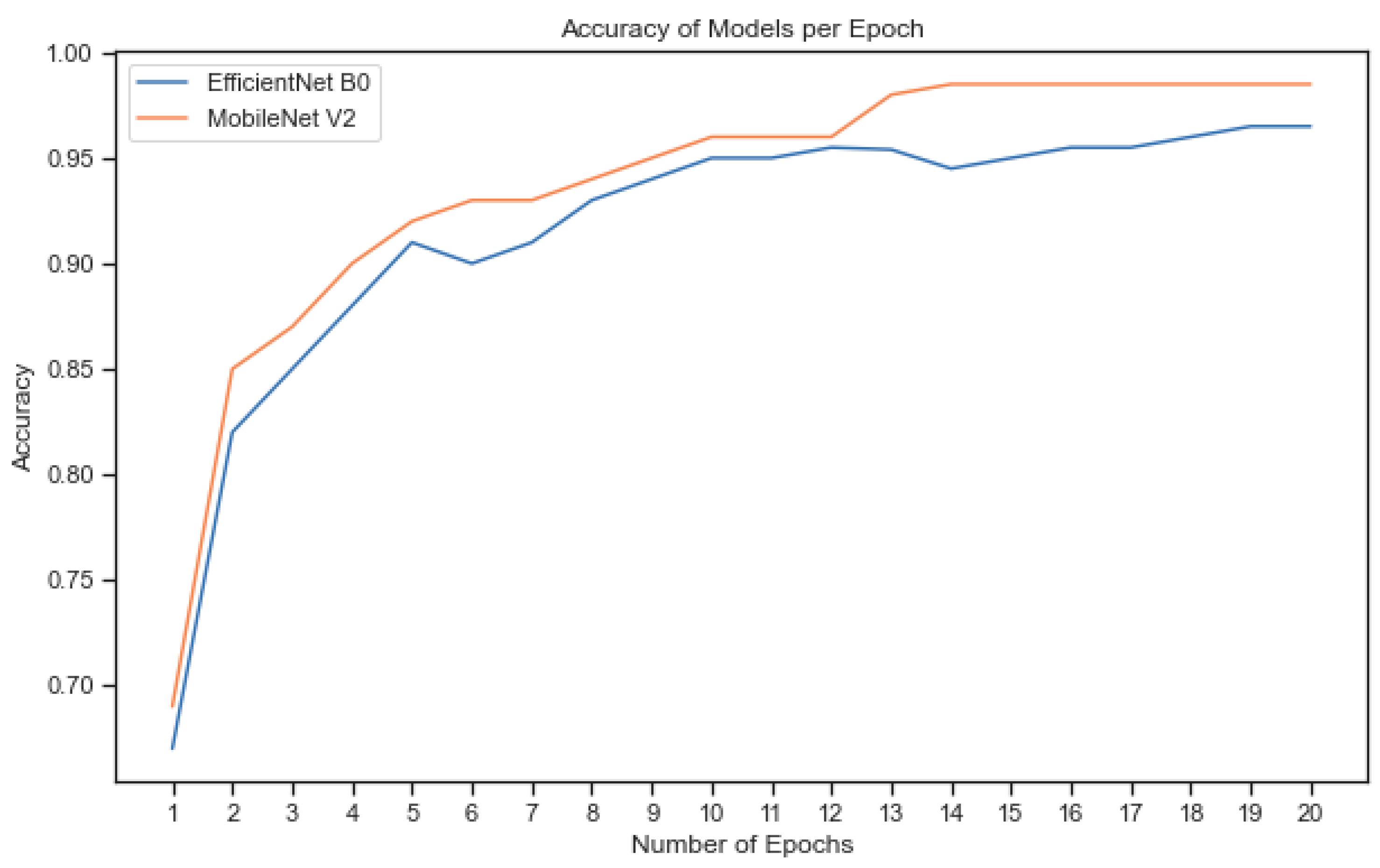
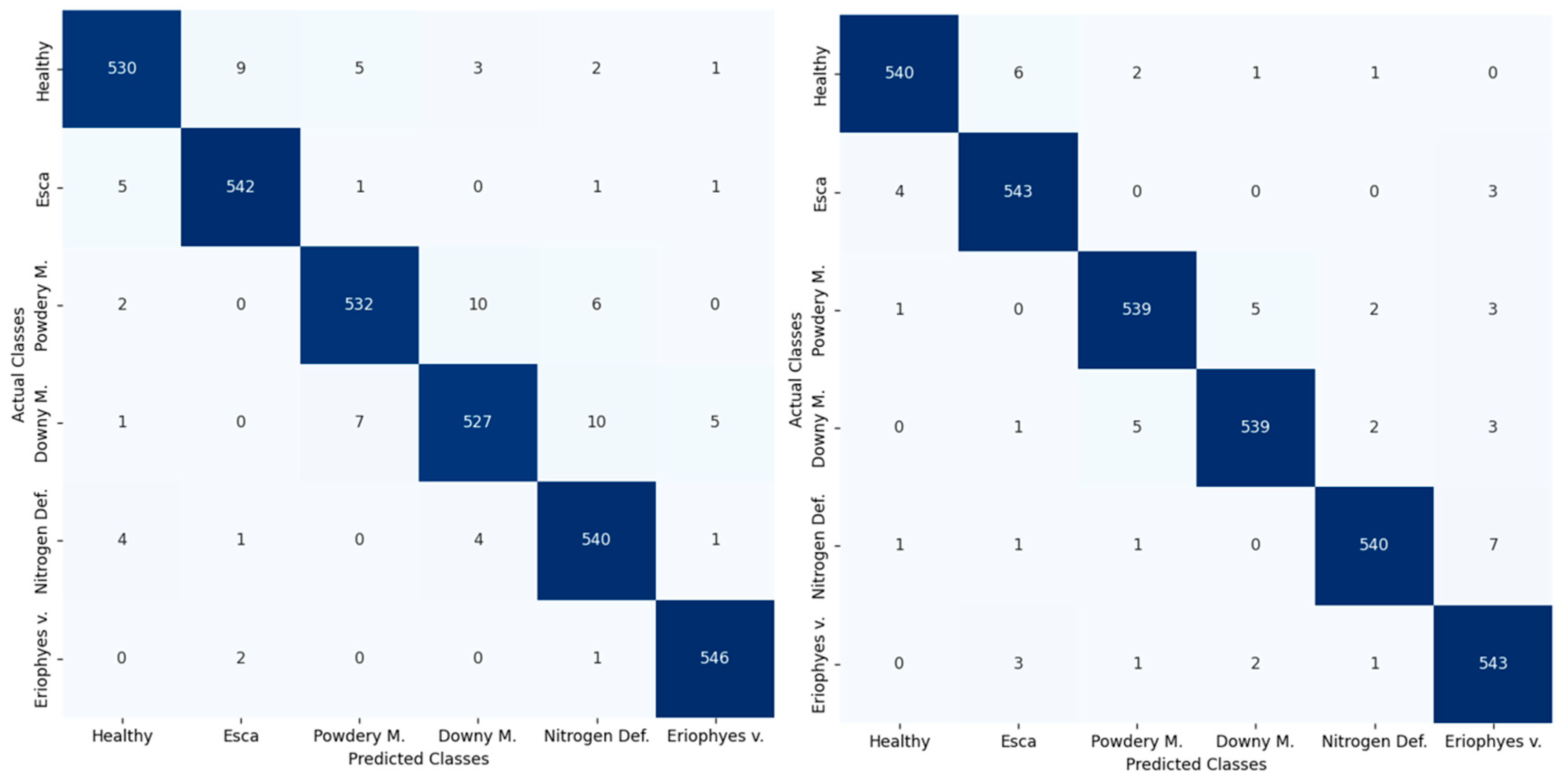
3.2. Transfer Learning Results

As was mentioned, the transfer learning approach that was followed in this work was the fine tuning of the whole convolutional base of both MobileNet V2 and EfficientNet B0.

Table 4. Validation accuracy results of the EfficientNet B0 and MobileNet V2, trained with the EdenLibrary dataset images, on the 20th training epoch.

	EfficientNet B0	MobileNet V2
Validation accuracy	0.965	0.985
F1 score	0.958	0.983

illustrates the validation accuracy and the F1 score of the two DL models, which were developed and trained with fine tuning using the EdenLibrary grapevines dataset. The values refer to the average of the classification process (average from all six classes). It is apparent that both of the models had an excellent detection performance for the possible health status of the plants. MobileNet V2 has a slightly better performance when compared to the EfficientNet B0. Additionally, the F1 scores are almost identical to the validation accuracy results, with less than 1% difference between the two metrics. This validates the balance between the training data from the six classes that were discussed.

Figure 9 depicts the accuracy performance of each of the two DL models in the validation phase, per epoch, of the fine-tuning process. From this figure it can be concluded that the higher performance of the MobileNet V2 network, in comparison with the EfficientNet B0 is observed even from the first epoch of the training and is maintained until the end of the training phase in the 20th epoch.

Additionally, MobileNet V2 has succeeded in converging to the maximum accuracy faster than EfficientNet B0. Furthermore, it is noteworthy that both models reached a high accuracy even before the completion of the fifth epoch. This indicates that the DL models were successful in quickly learning the patterns and features presented in the Eden Library dataset, demonstrating their ability to generalise well and make accurate predictions, even in early stages of the training process. Finally, the performance of each class in the training phase for both of the models is described in Figure 10.

The results shown in Figure 10 validate the good performance of both DL models in accurately distinguishing between the different health status classes. It is noteworthy that all classes have equal performance, and there is no class with extreme misclassified instances. Additionally, the spread of the misclassified instances is not biased as the misclassified examples are detected in the rest of the classes and not in a specific class.

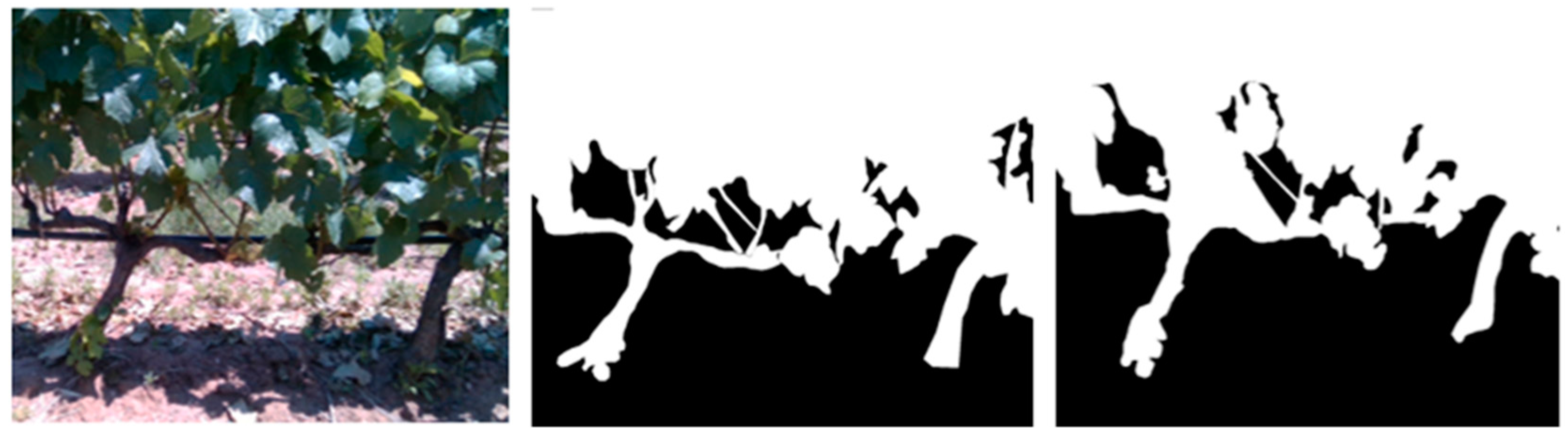
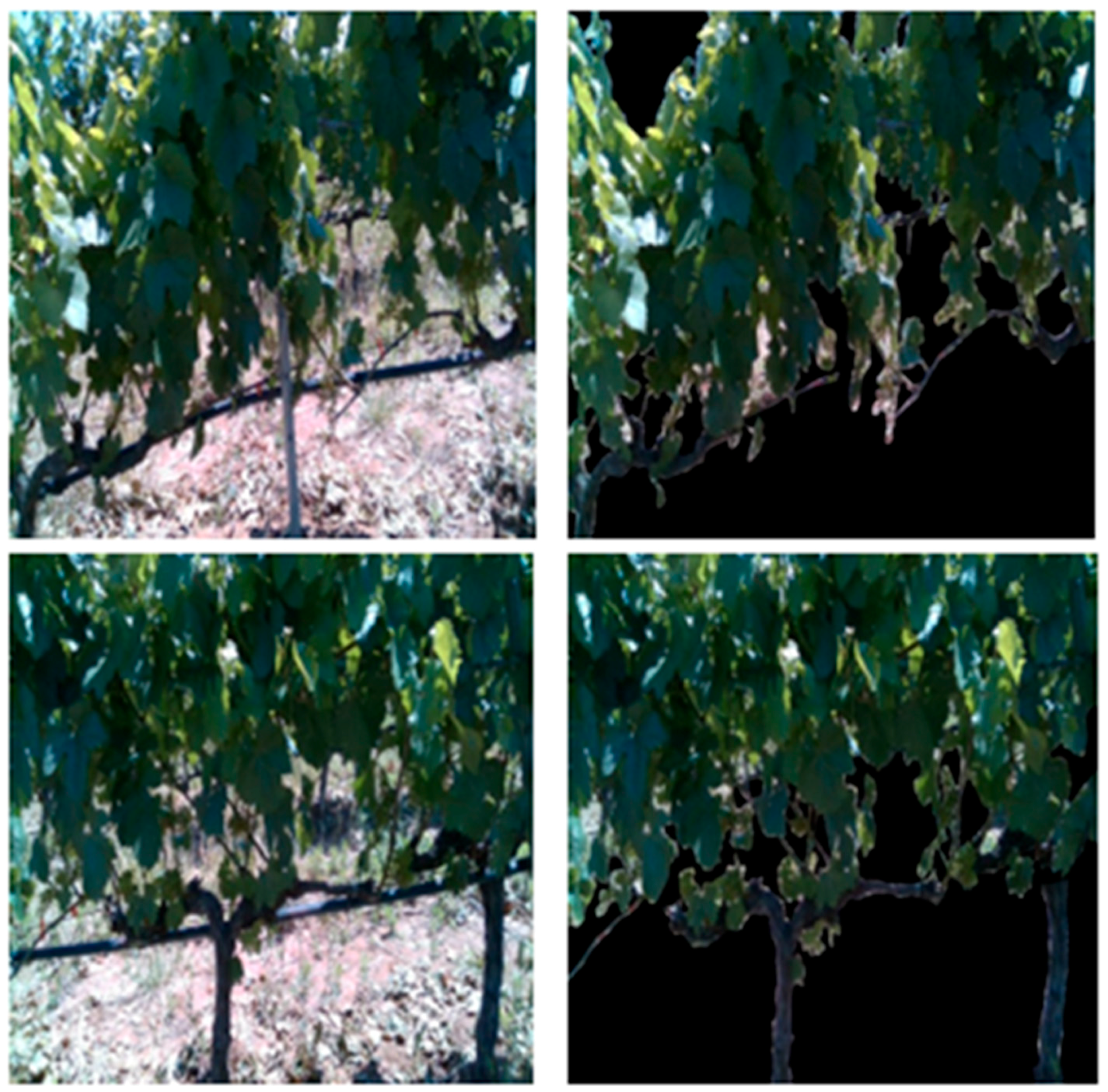
3.3. Semantic Segmentation Results

Training of the Mobile-UNet was performed using photos that were taken by a grapevine row in the field which was located close to the one where the measurements took place. The image acquisition was performed using the PiCamera mounted on the RPi, while the whole system was on a robotic platform The Mobile-UNet algorithm was also subjected to post-training quantization before being implemented for online detection in order to further reduce its computational requirements. To compare the performance of the segmentation given by the Mobile-UNet algorithm, ground truth data were created and compared with the output of the model in terms of IoU and F1 score. The segmentation performance of the proposed Mobile-UNet algorithm is given in

Table 5. Mobile-UNet segmentation in field performance on grapevines for the exclusion of the background.

Evaluation Metric	Mobile-UNet Performance
F1 score	0.82
IoU	0.79

.

From the results of Table 5, it can be concluded that the Mobile-UNet has successfully detected the region of interest. Most of the grapevine plants features in the captured images have been successfully included in the segmented images. An example of the Mobile-UNet’s performance on the test data is depicted in Figure 11.

From Figure 11, it is apparent that most of the segmentation error occurs in the inclusion of pixels that belong to the background rather than in pixels that belong to the plant that was being examined. Indeed, this can be also found in Figure 12, which shows how the segmented mask was applied on the photos from the video stream, and there are only a few spots with mainly green background pixels included to the foreground. Nevertheless, the segmented image includes all the regions of interest and excludes most of the background noise that could cause misclassification when the image will proceed to the DL algorithms for the health status assessment.

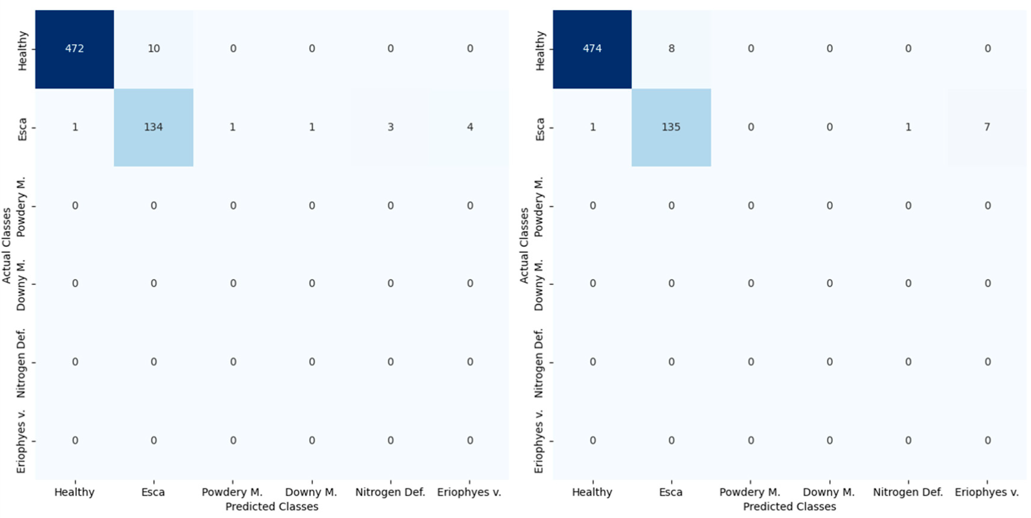
3.4. Online Validation of the Models

The segmented images from the grapevine plants that have been produced by the Mobile-UNet segmentation algorithm proceed to the fine-tuned DL models in order for them to be characterised as either healthy or infected. As was already mentioned, the validation of the models was performed in parts of four rows from the Chatzivariti winery (two from each of the different variety fields), where there were visible symptoms of esca in the grapevine plants, as was proposed by the plant pathologists.

The image acquisition in this study was performed with the RGB camera that was mounted on the RPi platform, facing directly on the grapevine plants. The whole system was recording for approximately 50 s, covering a row of almost 65 m, while there were two runs per row in order to deploy both of the DL models that were examined (MobileNet V2 and EfficientNet B0). The average accuracy results, as well as the models’ inference time for the validation phase of the whole system, is shown in

Table 6. Validation accuracy results and inference time of the proposed deep learning models with online deployment on the grapevine plants from Chatzivariti’s winery.

	EfficientNet B0	MobileNet V2
Validation accuracy	0.924	0.941
F1 score	0.949	0.961
Inference Time [ms]	390	330

.

Table 6 illustrates a discernible drop in accuracy across the board for both models when they were validated on the Chatzivariti winery. These results demonstrate the high effectiveness of both models in accurately classifying the incoming images. MobileNet, with its lightweight architecture and efficient design, has proven to be highly adept at recognising and categorising diseases in field conditions. Its remarkable accuracy of 0.941 indicates that it can reliably make correct predictions in a wide range of scenarios. On the other hand, EfficientNet B0, also had a very high performance, with an accuracy of 0.924. It should be noted that the evaluation metrics are calculated as if it was a binary classification problem with only the healthy and Esca class; this is due to too few instances in most classes. The higher F1 score that is reported is most likely due to the high imbalance between the different classes, as can be also validated by Figure 13.

As mentioned previously, the data used for the validation stage included healthy and esca-infected plants. Classes also exhibit imbalances as the real-world data had far more healthy plants than infected, as would be expected. Nevertheless, the algorithms performed excellently in each case, with only a small drop of around 5% in validation accuracy. That is further shown in the classification of each class (Figure 13), where the healthy status was correctly predicted, while the few misclassified Esca observations, especially in the case of MobileNet v2, were mainly attributed to the Eriophyes v. class. This may be a result of similarities in the leaf textures caused by the two different diseases.

The total inference time for both models was less than 400 ms (Table 6). Specifically, MobileNet V2 had a slightly faster inference, in comparison with the EfficientNet B0. It should be noted that this is the total inference time for the whole pipeline, from the input of the image through the output decision, which also includes the semantic segmentation algorithm with the Mobile-UNet, which is a time-consuming process. Nevertheless, the inference time of 330 ms for the MobileNet V2 corresponds to an effective frame rate of almost 3 FPS (3.03), which was the selected input frame rate in this study. On the other hand, the inference time for the EfficientNet B0 (390 ms) corresponds to an effective frame rate capacity of less than 3 FPS (2.63).

3.5. Web Based Service for Online Monitoring

MobileNet V2 was chosen as the best performing model for deployment in a web-based service. In this study, the service was deployed locally. The modern, rapid (high-performance) web framework Fast API was utilised to develop the API interface. Two endpoints have been established, as can be seen in Figure 14. The first endpoint is a GET request that returns a response message about the user’s name. The second endpoint /show_prediction is a POST request that takes as input images from the video stream and returns a .JSON output with details about the disease prediction and the location of the plants (Figure 14).

In order to make the service accessible to the end user, a Web interface needs to be developed using the React framework. This way, the user will be able to provide input by using the camera of Raspberry Pi, and the application will use the API developed in the previous step to forecast the plant health status.

4. Discussion

The objective of this research is to demonstrate an automated approach for disease detection in agriculture. The research focused on utilising pre-existing datasets from online libraries for the original training of DL models and apply a transfer learning approach for disease detection on real-life conditions in a winery estate. This approach was proven to be successful, with accuracy of more than 0.9 in both training and validation, which is in accordance with Ouhami et al. (2020) and Hasan et al. (2019), who have used a TL approach in their study for disease detection in tomato leaves [74,75]. They have also used pre-trained DL models (VGG16 and Inception v3 respectively), but these are not suitable for online deployment in edge devices given the performance requirements of the RPi. Aravind et al. (2020) have used smartphone images from four crops and succeeded with a validation accuracy of 0.9 on the online validation, using the VGG16 model [76].

Image segmentation with Mobile-UNet successfully preserved the regions of interest, i.e., the plant leaves, while omitting most of the background noise. As it was mentioned, U-Net is a widely used model for semantic segmentation due to its unique architecture, but it requires higher computational power than the RPi can give. Indeed, modified versions of U-Net have been used for the segmentation of leaves diseases by Zhang and Zhang (2023) [77] and Liu et al. (2022) [78]. Their results are evaluated offline, however, in contrast with what has been proposed in this study. As of the time of the writing of this paper, the performance of the Mobile-UNet has not been evaluated in the agricultural sector. The use of a different segmentation method, such as the depth dimension for faster inference of the models, should be considered for a future study.

The DL models that have been employed in this study were the EfficientNet B0 and the MobileNet V2. Their high performance in DL tasks and their high efficiency in terms of computational power, due to their lightweight architecture, made them suitable choices for online deployment. Table 6 shows that the obtained accuracies of 0.94 and 0.92 for MobileNet V2 and EfficientNet B0 respectively showcase the strong predictive capabilities of these models when applied to real-world data. These results are almost in accordance with what Bir et al. (2020) have found in their study on tomato leaves, where the two models have shown comparable results as well, but EfficientNet B0 outperformed MobileNet V2, by a very small amount (0.4%) [79]. Regarding the validation performance of the DL models, it was in general slightly lower than in the training. This should not come as unexpected as the models were initially trained and validated on the same dataset (Eden Library) and the new data from the field may cause the models to not accurately detect all the features the same way they did with the training set.

Model evaluation in real-world conditions was achieved by importing the models with an RPi device that uses a camera module to capture RGB images from the video stream. Those images are processed by the DL models in the RPi and outputs the result, which, in turn, is transmitted through fastAPI in a web service interface, as is also shown by Sharma et al. (2022), who have developed a web-based service that takes tomato leaf images as an input and performs disease detection [80]. In parallel, the RPi can be integrated in a robotic platform using ROS and, through ROS nodes, can receive a different input from an RGB camera topic, mounted on a UGV, and transmit the decision output to the developed web service along with various other messages from other sensors in the robotic platform, depending on the configuration. In this work, the ROS node was not tested online.

Certain limitations apply for this use case. While there are more powerful sensors, such as hyperspectral cameras [81], that capture more information from the electromagnetic spectrum than RGB, these are usually commercial, licensed products. The same considerations apply for the software used to create the models. This makes the use of open-source software a necessity. For this reason, this research used python as a programming language for the algorithms and a Linux distribution as the RPi’s operating system to deploy the models.

While this research focused on grapevine plants and, specifically, diseases affecting their leaves, it is important to note that this approach should be primarily validated in the other disease classes on which the models have been trained, not only in Esca, and can also be extended to detect diseases in other types of crops. Moreover, research can be focused on different types of disease, affecting fruits of the plants or, in the case of grapevines, their grapes. Botrytis cinerea is a pathogen affecting more than 200 crops worldwide. In the case of grapevines, visual symptoms are observable on the grapes. Another possible approach is the detection of pests and insects that can allow for an even earlier warning about crop safety before the disease causes visible symptoms.

5. Conclusions

The present study focuses on an IoT approach to disease detection in grapevine plants in field conditions by implementing deep learning (DL) algorithms, trained under the transfer learning (TL) technique and using commercially available data sets.

Firstly, this study demonstrates the effective use of TL in adapting pretrained DL models to the context of grapevine disease detection. This approach strikes a balance between model efficiency and computational requirements, enabling the deployment of lightweight models on edge devices like the Raspberry Pi while maintaining high accuracy.

Additionally, the Mobile-UNet was successfully implemented for real-time segmentation of plants from their background, with a high intersection over union (IoU) accuracy and fast inference times, which play a crucial role in the generation of the final model’s decision.

Among the DL models considered, MobileNet has been identified as the optimal algorithm for disease detection in this study. It has showcased superior performance while necessitating lower power and memory resources. As a result, MobileNet enables real-time disease detection with the designated frame rate of the RGB camera, contributing to efficient and timely results.

This study goes beyond traditional disease detection by integrating the DL models into an IoT framework that can be further connected to robotic platforms, using ROS, for automated, real-time monitoring and response systems in agriculture.

Emphasizing the use of open-source software and commercially available datasets, this research addresses the practical constraints of agricultural technology deployment, making it accessible and replicable.

In conclusion, this research not only highlights the feasibility of employing IoT devices with modest power and memory requirements for the real-time detection of grapevine diseases under field conditions, it also introduces novel methodologies and integrations that have the potential to significantly advance disease monitoring and management in the grapevine industry and beyond.

References

1. Robertson, G.P.; Swinton, S.M. Reconciling agricultural productivity and environmental integrity: A grand challenge for agriculture. Front. Ecol. Environ. 2005, 3, 38–46. [Google Scholar] [CrossRef]
2. Morellos, A.; Tziotzios, G.; Orfanidou, C.; Pantazi, X.E.; Sarantaris, C.; Maliogka, V.; Alexandridis, T.K.; Moshou, D. Non-destructive early detection and quantitative severity stage classification of Tomato Chlorosis Virus (ToCV) infection in young tomato plants using vis–NIR Spectroscopy. Remote Sens. 2020, 12, 1920. [Google Scholar] [CrossRef]
3. Anderson, P.K.; Cunningham, A.A.; Patel, N.G.; Morales, F.J.; Epstein, P.R.; Daszak, P. Emerging infectious diseases of plants: Pathogen pollution, climate change and agrotechnology drivers. Trends Ecol. Evol. 2004, 19, 535–544. [Google Scholar] [CrossRef] [PubMed]
4. Desprez-Loustau, M.-L.; Robin, C.; Buee, M.; Courtecuisse, R.; Garbaye, J.; Suffert, F.; Sache, I.; Rizzo, D.M. The fungal dimension of biological invasions. Trends Ecol. Evol. 2007, 22, 472–480. [Google Scholar] [CrossRef]
5. Fisher, M.C.; Henk, D.A.; Briggs, C.J.; Brownstein, J.S.; Madoff, L.C.; McCraw, S.L.; Gurr, S.J. Emerging fungal threats to animal, plant and ecosystem health. Nature 2012, 484, 186–194. [Google Scholar] [CrossRef]
6. Ristaino, J.B.; Records, A. Emerging Plant Diseases and Global Food Security; American Phytopathological Society: St. Paul, MN, USA, 2020. [Google Scholar]
7. Lampridi, M.G.; Sørensen, C.G.; Bochtis, D. Agricultural Sustainability: A Review of Concepts and Methods. Sustainability 2019, 11, 5120. [Google Scholar] [CrossRef]
8. Giraud, T.; Gladieux, P.; Gavrilets, S. Linking the emergence of fungal plant diseases with ecological speciation. Trends Ecol. Evol. 2010, 25, 387–395. [Google Scholar] [CrossRef] [PubMed]
9. Gladieux, P.; Feurtey, A.; Hood, M.E.; Snirc, A.; Clavel, J.; Dutech, C.; Roy, M.; Giraud, T. The population biology of fungal invasions. In Invasion Genetics: The Baker and Stebbins Legacy; John Wiley & Sons, Ltd.: Hoboken, NJ, USA, 2016; pp. 81–100. [Google Scholar]
10. Fontaine, M.C.; Labbé, F.; Dussert, Y.; Delière, L.; Richart-Cervera, S.; Giraud, T.; Delmotte, F. Europe as a bridgehead in the worldwide invasion history of grapevine downy mildew, Plasmopara viticola. Curr. Biol. 2021, 31, 2155–2166. [Google Scholar] [CrossRef]
11. Thind, T.S.; Arora, J.K.; Mohan, C.; Raj, P. Epidemiology of powdery mildew, downy mildew and anthracnose diseases of grapevine. In Diseases of Fruits and Vegetables Volume I; Springer: Dordrecht, The Netherlands, 2004; pp. 621–638. [Google Scholar]
12. Da Silva, C.M.; Schwan-Estrada, K.R.F.; Rios, C.M.F.D.; Batista, B.N.; Pascholati, S.F. Effect of culture filtrate of Curvularia inaequalis on disease control and productivity of grape cv. Isabel. Afr. J. Agric. Res. 2014, 9, 3001–3010. [Google Scholar]
13. Berdugo, C.A.; Mahlein, A.-K.; Steiner, U.; Dehne, H.-W.; Oerke, E.-C. Sensors and imaging techniques for the assessment of the delay of wheat senescence induced by fungicides. Funct. Plant Biol. 2013, 40, 677–689. [Google Scholar] [CrossRef]
14. Weissteiner, C.J.; Pistocchi, A.; Marinov, D.; Bouraoui, F.; Sala, S. An indicator to map diffuse chemical river pollution considering buffer capacity of riparian vegetation—A pan-European case study on pesticides. Sci. Total Environ. 2014, 484, 64–73. [Google Scholar] [CrossRef] [PubMed]
15. Zhang, X.; Wen, Q.; Tian, D.; Hu, J. PVIDSS: Developing a WSN-based irrigation decision support system (IDSS) for viticulture in protected area, Northern China. Appl. Math. Inf. Sci. 2015, 9, 669. [Google Scholar]
16. Zhao, Y.Y.; Pei, Y.S. Risk evaluation of groundwater pollution by pesticides in China: A short review. Procedia Environ. Sci. 2012, 13, 1739–1747. [Google Scholar] [CrossRef]
17. Huang, Z.; Qin, A.; Lu, J.; Menon, A.; Gao, J. Grape leaf disease detection and classification using machine learning. In Proceedings of the 2020 International Conferences on Internet of Things (iThings) and IEEE Green Computing and Communications (GreenCom) and IEEE Cyber, Physical and Social Computing (CPSCom) and IEEE Smart Data (SmartData) and IEEE Congress on Cybermatics (Cybermatics), Rhodes, Greece, 2–6 November 2020; pp. 870–877. [Google Scholar]
18. Ali, M.M.; Bachik, N.A.; Muhadi, N.; Yusof, T.N.T.; Gomes, C. Non-destructive techniques of detecting plant diseases: A review. Physiol. Mol. Plant Pathol. 2019, 108, 6. [Google Scholar] [CrossRef]
19. Mulla, D.J. Twenty five years of remote sensing in precision agriculture: Key advances and remaining knowledge gaps. Biosyst. Eng. 2013, 114, 358–371. [Google Scholar] [CrossRef]
20. Liakos, K.G.; Busato, P.; Moshou, D.; Pearson, S.; Bochtis, D. Machine learning in agriculture: A review. Sensors 2018, 18, 2674. [Google Scholar] [CrossRef] [PubMed]
21. Benos, L.; Tagarakis, A.C.; Dolias, G.; Berruto, R.; Kateris, D.; Bochtis, D. Machine learning in agriculture: A comprehensive updated review. Sensors 2021, 21, 3758. [Google Scholar] [CrossRef]
22. Di Gennaro, S.F.; Battiston, E.; di Marco, S.; Facini, O.; Matese, A.; Nocentini, M.; Palliotti, A.; Mugnai, L. Unmanned Aerial Vehicle (UAV)-based remote sensing to monitor grapevine leaf stripe disease within a vineyard affected by esca complex. Phytopathol. Mediterr. 2016, 55, 262–275. [Google Scholar] [CrossRef]
23. Wang, Y.M.; Ostendorf, B.; Pagay, V. Evaluating the Potential of High-Resolution Visible Remote Sensing to Detect Shiraz Disease in Grapevines. Aust. J. Grape Wine Res. 2023, 2023, 7376153. [Google Scholar] [CrossRef]
24. Cohen, B.; Edan, Y.; Levi, A.; Alchanatis, V. Early detection of grapevine (Vitis vinifera) downy mildew (Peronospora) and diurnal variations using thermal imaging. Sensors 2022, 22, 3585. [Google Scholar] [CrossRef]
25. Zia-Khan, S.; Kleb, M.; Merkt, N.; Schock, S.; Müller, J. Application of infrared imaging for early detection of Downy Mildew (Plasmopara viticola) in grapevine. Agriculture 2022, 12, 617. [Google Scholar] [CrossRef]
26. Bendel, N.; Backhaus, A.; Kicherer, A.; Köckerling, J.; Maixner, M.; Jarausch, B.; Biancu, S.; Klück, H.-C.; Seiffert, U.; Voegele, R.T. Detection of two different grapevine yellows in Vitis vinifera using hyperspectral imaging. Remote Sens. 2020, 12, 4151. [Google Scholar] [CrossRef]
27. Gao, Z.; Khot, L.R.; Naidu, R.A.; Zhang, Q. Early detection of grapevine leafroll disease in a red-berried wine grape cultivar using hyperspectral imaging. Comput. Electron. Agric. 2020, 179, 7. [Google Scholar] [CrossRef]
28. Junges, A.H.; Ducati, J.R.; Lampugnani, C.S.; Almança, M.A.K. Detection of grapevine leaf stripe disease symptoms by hyperspectral sensor. Phytopathol. Mediterr. 2018, 57, 399–406. [Google Scholar]
29. Anagnostis, A.; Tagarakis, A.C.; Asiminari, G.; Papageorgiou, E.; Kateris, D.; Moshou, D.; Bochtis, D. A deep learning approach for anthracnose infected trees classification in walnut orchards. Comput. Electron. Agric. 2021, 182, 105998. [Google Scholar] [CrossRef]
30. Anagnostis, A.; Asiminari, G.; Papageorgiou, E.; Bochtis, D. A convolutional neural networks based method for anthracnose infected walnut tree leaves identification. Appl. Sci. 2020, 10, 469. [Google Scholar] [CrossRef]
31. Tarek, H.; Aly, H.; Eisa, S.; Abul-Soud, M. Optimized deep learning algorithms for tomato leaf disease detection with hardware deployment. Electronics 2022, 11, 140. [Google Scholar] [CrossRef]
32. He, K.; Zhang, X.; Ren, S.; Sun, J. Deep residual learning for image recognition. In Proceedings of the IEEE Conference on Computer Vision and Pattern Recognition, Las Vegas, NV, USA, 26 June–1 July 2016; pp. 770–778. [Google Scholar]
33. LeCun, Y.; Bottou, L.; Bengio, Y.; Haffner, P. Gradient-based learning applied to document recognition. In Proceedings of the IEEE; IEEE: New York, NY, USA, 1998; Volume 86, pp. 2278–2324. [Google Scholar]
34. Monien, B.; Preis, R.; Schamberger, S.; Gonzalez, T. Approximation algorithms for multilevel graph partitioning. Handb. Approx. Algorithms Metaheuristics 2007, 10, 1–60. [Google Scholar]
35. Chen, H.; Wang, Y.; Guo, T.; Xu, C.; Deng, Y.; Liu, Z.; Ma, S.; Xu, C.; Xu, C.; Gao, W. Pre-trained image processing transformer. In Proceedings of the IEEE/CVF Conference on Computer Vision and Pattern Recognition, Virtual, 19–25 June 2021; pp. 12299–12310. [Google Scholar]
36. Lee, S.; Jeong, Y.; Son, S.; Lee, B. A self-predictable crop yield platform (SCYP) based on crop diseases using deep learning. Sustainability 2019, 11, 3637. [Google Scholar] [CrossRef]
37. Saleem, M.H.; Potgieter, J.; Arif, K.M. Plant disease detection and classification by deep learning. Plants 2019, 8, 468. [Google Scholar] [CrossRef] [PubMed]
38. Sharma, A.; Chandak, A.; Khandelwal, A.; Gandhi, R. Detection of Diseases in Tomato Plant using Machine Learning. Int. J. Next-Gener. Comput. 2022, 13, 942. [Google Scholar]
39. Gutiérrez, S.; Hernández, I.; Ceballos, S.; Barrio, I.; Díez-Navajas, A.M.; Tardaguila, J. Deep learning for the differentiation of downy mildew and spider mite in grapevine under field conditions. Comput. Electron. Agric. 2021, 182, 1. [Google Scholar] [CrossRef]
40. Alessandrini, M.; Rivera, R.C.F.; Falaschetti, L.; Pau, D.; Tomaselli, V.; Turchetti, C. A grapevine leaves dataset for early detection and classification of esca disease in vineyards through machine learning. Data Brief 2021, 35, 9. [Google Scholar] [CrossRef] [PubMed]
41. Ribani, R.; Marengoni, M. A survey of transfer learning for convolutional neural networks. In Proceedings of the 2019 32nd SIBGRAPI Conference on Graphics, Patterns and Images Tutorials (SIBGRAPI-T), Rio de Janeiro, Brazil, 28–31 October 2019; pp. 47–57. [Google Scholar]
42. Pan, S.J.; Yang, Q. A survey on transfer learning. IEEE Trans. Knowl. Data Eng. 2009, 22, 1345–1359. [Google Scholar] [CrossRef]
43. Morellos, A.; Pantazi, X.E.; Paraskevas, C.; Moshou, D. Comparison of Deep Neural Networks in Detecting Field Grapevine Diseases Using Transfer Learning. Remote Sens. 2022, 14, 4648. [Google Scholar] [CrossRef]
44. Brahimi, M.; Boukhalfa, K.; Moussaoui, A. Deep learning for tomato diseases: Classification and symptoms visualization. Appl. Artif. Intell. 2017, 31, 299–315. [Google Scholar] [CrossRef]
45. Nigam, S.; Jain, R.; Marwaha, S.; Arora, A.; Haque, M.A.; Dheeraj, A.; Singh, V.K. Deep transfer learning model for disease identification in wheat crop. Ecol. Inform. 2023, 75, 8. [Google Scholar] [CrossRef]
46. Liu, B.; Zhang, Y.; He, D.; Li, Y. Identification of apple leaf diseases based on deep convolutional neural networks. Symmetry 2017, 10, 11. [Google Scholar] [CrossRef]
47. Gobhinath, S.; Darshini, M.D.; Durga, K.; Priyanga, R.H. Smart irrigation with field protection and crop health monitoring system using autonomous rover. In Proceedings of the 2019 5th International Conference on Advanced Computing & Communication Systems (ICACCS), Coimbatore, India, 15–16 March 2019; pp. 198–203. [Google Scholar]
48. Pawar, S.B.; Rajput, P.; Shaikh, A. Smart irrigation system using IOT and raspberry pi. Int. Res. J. Eng. Technol. 2018, 5, 1163–1166. [Google Scholar]
49. Athani, S.; Tejeshwar, C.H.; Patil, M.M.; Patil, P.; Kulkarni, R. Soil moisture monitoring using IoT enabled arduino sensors with neural networks for improving soil management for farmers and predict seasonal rainfall for planning future harvest in North Karnataka—India. In Proceedings of the 2017 International Conference on I-SMAC (IoT in Social, Mobile, Analytics and Cloud) (I-SMAC), Palladam, India, 10–11 February 2017; pp. 43–48. [Google Scholar]
50. Postolache, S.; Sebastião, P.; Viegas, V.; Postolache, O.; Cercas, F. IoT-Based Systems for Soil Nutrients Assessment in Horticulture. Sensors 2022, 23, 403. [Google Scholar] [CrossRef] [PubMed]
51. Venkatesan, R.; Kathrine, G.J.W.; Ramalakshmi, K. Internet of Things based pest management using natural pesticides for small scale organic gardens. J. Comput. Theor. Nanosci. 2018, 15, 2742–2747. [Google Scholar] [CrossRef]
52. Pantazi, X.E.; Moshou, D.; Oberti, R.; West, J.; Mouazen, A.M.; Bochtis, D. Detection of biotic and abiotic stresses in crops by using hierarchical self organizing classifiers. Precis. Agric. 2017, 18, 383–393. [Google Scholar] [CrossRef]
53. Pantazi, X.E.; Moshou, D.; Bochtis, D. Intelligent Data Mining and Fusion Systems in Agriculture; Academic Press: Cambridge, MA, USA, 2019; ISBN 9780128143926. [Google Scholar]
54. Mishra, M.; Choudhury, P.; Pati, B. Modified ride-NN optimizer for the IoT based plant disease detection. J. Ambient. Intell. Humaniz. Comput. 2021, 12, 691–703. [Google Scholar] [CrossRef]
55. Brammya, G.; Antely, A.S. Face recognition using active appearance and type-2 fuzzy classifier. Multimed. Res 2019, 2, 1–8. [Google Scholar]
56. Kumar, V.S.; Gogul, I.; Raj, M.D.; Pragadesh, S.K.; Sebastin, J.S. Smart autonomous gardening rover with plant recognition using neural networks. Procedia Comput. Sci. 2016, 93, 975–981. [Google Scholar] [CrossRef]
57. Zhang, Z.; Wang, X.; Lai, Q.; Zhang, Z. Review of Variable-Rate Sprayer Applications Based on Real-Time Sensor Technologies. In Automation in Agriculture—Securing Food Supplies for Future Generations; Intech: Vienna, Austria, 2018. [Google Scholar]
58. Howard, A.G.; Zhu, M.; Chen, B.; Kalenichenko, D.; Wang, W.; Weyand, T.; Andreetto, M.; Adam, H. Mobilenets: Efficient convolutional neural networks for mobile vision applications. arXiv 2017, arXiv:1704.04861. [Google Scholar]
59. Szegedy, C.; Liu, W.; Jia, Y.; Sermanet, P.; Reed, S.; Anguelov, D.; Erhan, D.; Vanhoucke, V.; Rabinovich, A. Going deeper with convolutions. In Proceedings of the IEEE Conference on Computer Vision and Pattern Recognition, Boston, MA, USA, 7–12 June 2015; pp. 1–9. [Google Scholar]
60. Sandler, M.; Howard, A.; Zhu, M.; Zhmoginov, A.; Chen, L.-C. Mobilenetv2: Inverted residuals and linear bottlenecks. In Proceedings of the IEEE Conference on Computer Vision and Pattern Recognition, Salt Lake City, UT, USA, 18–22 June 2018; pp. 4510–4520. [Google Scholar]
61. Sifre, L.; Mallat, S. Rigid-motion scattering for texture classification. arXiv 2014, arXiv:1403.1687. [Google Scholar]
62. Iandola, F.N.; Han, S.; Moskewicz, M.W.; Ashraf, K.; Dally, W.J.; Keutzer, K. SqueezeNet: AlexNet-level accuracy with 50x fewer parameters and <0.5 MB model size. arXiv 2016, arXiv:1602.07360. [Google Scholar]
63. Tan, M.; Le, Q. Efficientnet: Rethinking model scaling for convolutional neural networks. In Proceedings of the 36th International Conference on Machine Learning, Long Beach, CA, USA, 10–15 June 2019; pp. 6105–6114. [Google Scholar]
64. Hu, J.; Shen, L.; Sun, G. Squeeze-and-excitation networks. In Proceedings of the IEEE Conference on Computer Vision and Pattern Recognition (CVPR 2018), Salt Lake City, UT, USA, 18–22 June 2018. [Google Scholar]
65. Li, B.; Liu, L.; Jin, Y.; Gao, P.; Sun, H.; Zheng, N. Designing Efficient Shortcut Architecture for Improving the Accuracy of Fully Quantized Neural Networks Accelerator. In Proceedings of the 2020 25th Asia and South Pacific Design Automation Conference (ASP-DAC), Beijing, China, 13–16 January 2020; pp. 289–294. [Google Scholar]
66. Qiu, J.; Wang, J.; Yao, S.; Guo, K.; Li, B.; Zhou, E.; Yu, J.; Tang, T.; Xu, N.; Song, S. Going deeper with embedded FPGA platform for convolutional neural network. In Proceedings of the 2016 ACM/SIGDA International Symposium on Field-Programmable Gate Arrays, Monterey, CA, USA, 21–23 February 2016; pp. 26–35. [Google Scholar]
67. Esser, S.K.; Merolla, P.A.; Arthur, J.V.; Cassidy, A.S.; Appuswamy, R.; Andreopoulos, A.; Berg, D.J.; McKinstry, J.L.; Melano, T.; Barch, D.R.; et al. Convolutional networks for fast, energy-efficient neuromorphic computing. Proc. Natl. Acad. Sci. USA 2016, 113, 11441–11446. [Google Scholar] [CrossRef]
68. Bao, Z.; Zhan, K.; Zhang, W.; Guo, J. LSFQ: A low precision full integer quantization for high-performance FPGA-based CNN acceleration. In Proceedings of the 2021 IEEE Symposium in Low-Power and High-Speed Chips (COOL CHIPS), Tokyo, Japan, 14–16 April 2021; pp. 1–6. [Google Scholar]
69. Ronneberger, O.; Fischer, P.; Brox, T. U-net: Convolutional networks for biomedical image segmentation. In Proceedings of the Lecture Notes in Computer Science (Including Subseries Lecture Notes in Artificial Intelligence and Lecture Notes in Bioinformatics); Springer: Cham, Switzerland, 2015. [Google Scholar]
70. Kumar, P.; Nagar, P.; Arora, C.; Gupta, A. U-segnet: Fully convolutional neural network based automated brain tissue segmentation tool. In Proceedings of the 2018 25th IEEE International Conference on Image Processing (ICIP), Athens, Greece, 7–10 October 2018; pp. 3503–3507. [Google Scholar]
71. Jing, J.; Wang, Z.; R”atsch, M.; Zhang, H. Mobile-Unet: An efficient convolutional neural network for fabric defect detection. Text. Res. J. 2022, 92, 30–42. [Google Scholar] [CrossRef]
72. Yu, J.; Zhang, J.; Shu, A.; Chen, Y.; Chen, J.; Yang, Y.; Tang, W.; Zhang, Y. Study of convolutional neural network-based semantic segmentation methods on edge intelligence devices for field agricultural robot navigation line extraction. Comput. Electron. Agric. 2023, 209, 1. [Google Scholar] [CrossRef]
73. Zou, K.; Chen, X.; Wang, Y.; Zhang, C.; Zhang, F. A modified U-Net with a specific data argumentation method for semantic segmentation of weed images in the field. Comput. Electron. Agric. 2021, 187, 2. [Google Scholar] [CrossRef]
74. Ouhami, M.; Es-Saady, Y.; El Hajji, M.; Hafiane, A.; Canals, R.; El Yassa, M. Deep transfer learning models for tomato disease detection. In Proceedings of the Lecture Notes in Computer Science (Including Subseries Lecture Notes in Artificial Intelligence and Lecture Notes in Bioinformatics); Springer: Cham, Switzerland, 2020; Volume 12119, pp. 65–73. [Google Scholar]
75. Hasan, M.; Tanawala, B.; Patel, K.J. Deep Learning Precision Farming: Tomato Leaf Disease Detection by Transfer Learning. SSRN Electron. J. 2019. [Google Scholar] [CrossRef]
76. Rangarajan Aravind, K.; Maheswari, P.; Raja, P.; Szczepański, C. Crop disease classification using deep learning approach: An overview and a case study. In Deep Learning for Data Analytics: Foundations, Biomedical Applications, and Challenges; Academic Press: Cambridge, MA, USA, 2020; pp. 173–195. ISBN 9780128197646. [Google Scholar]
77. Zhang, S.; Zhang, C. Modified U-Net for plant diseased leaf image segmentation. Comput. Electron. Agric. 2023, 204, 1. [Google Scholar] [CrossRef]
78. Liu, W.; Yu, L.; Luo, J. A hybrid attention-enhanced DenseNet neural network model based on improved U-Net for rice leaf disease identification. Front. Plant Sci. 2022, 13, 9. [Google Scholar] [CrossRef] [PubMed]
79. Bir, P.; Kumar, R.; Singh, G. Transfer learning based tomato leaf disease detection for mobile applications. In Proceedings of the 2020 IEEE International Conference on Computing, Power and Communication Technologies, Greater Noida, India, 2–4 October 2020; pp. 34–39. [Google Scholar]
80. Sharma, A.; Kukreja, V.; Bansal, A.; Mahajan, M. Multi classification of Tomato Leaf Diseases: A Convolutional Neural Network Model. In Proceedings of the 2022 10th International Conference on Reliability, Infocom Technologies and Optimization (Trends and Future Directions), Noida, India, 13–14 October 2022; pp. 1–5. [Google Scholar]
81. Adão, T.; Hruška, J.; Pádua, L.; Bessa, J.; Peres, E.; Morais, R.; Sousa, J.J. Hyperspectral imaging: A review on UAV-based sensors, data processing and applications for agriculture and forestry. Remote Sens. 2017, 9, 1110. [Google Scholar] [CrossRef]
Figure 1. Sample dataset images that belong to the grapevines subset from the Eden Library dataset.
Applsci 14 01049 g001
Figure 2. The Chatzivariti winery location within northern Greece (left) and the survey fields (right). The Xinomavro and Negoska varieties field (field 1) is located in the south, and the Traminer variety field (field 2) is located in the north.
Applsci 14 01049 g002
Figure 3. High-level architecture of The MobileNet V2 model.
Applsci 14 01049 g003
Figure 4. The EfficientNet B0 architecture.
Applsci 14 01049 g004
Figure 5. Raspberry Pi 4 model B. The barebone configuration (left) and RPi in the steel case, mounted with Camera and GPS modules (right).
Applsci 14 01049 g005
Figure 6. High-level architecture of the Mobile-UNet segmentation model.
Applsci 14 01049 g006
Figure 7. A close-up (left) and a distant photo (righttop) of the proposed Raspberry Pi integrated system, with the RGB camera, for the online disease detection on grapevine plants, placed on the UGV and a photo during the online measurements on the field (rightbottom).
Applsci 14 01049 g007
Figure 8. Architecture of the overall system design, comprising the DL models, the RPi4/UGV hardware, and the IoT output decision.
Applsci 14 01049 g008
Figure 9. Validation accuracy in the different training epochs for the two different pretrained models.
Applsci 14 01049 g009
Figure 10. Confusion matrix of the classification results of EfficientNet B0 (left) and MobileNet V2 (right) during the training phase.
Applsci 14 01049 g010
Figure 11. Example of Mobile-UNet’s performance on the online segmentation of the grapevine from its background surrounding. Left: the original image, as was captured by the RGB camera; Middle: the ground truth mask that was used for the evaluation; and Right: the segmentation mask, as it was produced by the Mobile-UNet algorithm.
Applsci 14 01049 g011
Figure 12. Application of the segmented mask by the Mobile-UNet algorithm on the photos that were captured during the field survey.
Applsci 14 01049 g012
Figure 13. Confusion Matrix of EfficientNet B0 (left) and MobileNet V2 (right) during the online validation.
Applsci 14 01049 g013
Figure 14. FastAPI Interface (Swagger API).
Applsci 14 01049 g014