Optimizing Cybersecurity Attack Detection in Computer Networks: A Comparative Analysis of Bio-Inspired Optimization Algorithms Using the CSE-CIC-IDS 2018 Dataset

Abstract

In computer network security, the escalating use of computer networks and the corresponding increase in cyberattacks have propelled Intrusion Detection Systems (IDSs) to the forefront of research in computer science. IDSs are a crucial security technology that diligently monitor network traffic and host activities to identify unauthorized or malicious behavior. This study develops highly accurate models for detecting a diverse range of cyberattacks using the fewest possible features, achieved via a meticulous selection of features. We chose 5, 9, and 10 features, respectively, using the Artificial Bee Colony (ABC), Flower Pollination Algorithm (FPA), and Ant Colony Optimization (ACO) feature-selection techniques. We successfully constructed different models with a remarkable detection accuracy of over 98.8% (approximately 99.0%) with Ant Colony Optimization (ACO), an accuracy of 98.7% with the Flower Pollination Algorithm (FPA), and an accuracy of 98.6% with the Artificial Bee Colony (ABC). Another achievement of this study is the minimum model building time achieved in intrusion detection, which was equal to 1 s using the Flower Pollination Algorithm (FPA), 2 s using the Artificial Bee Colony (ABC), and 3 s using Ant Colony Optimization (ACO). Our research leverages the comprehensive and up-to-date CSE-CIC-IDS2018 dataset and uses the preprocessing Discretize technique to discretize data. Furthermore, our research provides valuable recommendations to network administrators, aiding them in selecting appropriate machine learning algorithms tailored to specific requirements.

1. Introduction

Large-scale local area networks use anomaly detection as a primary technique for solving security issues. However, it can be challenging to extract accurate traffic data for anomaly identification [1]. Intrusion detection in computer networks is crucial as it affects communication and security; yet, finding network intrusions remains a challenge [1]. Network intrusion detection is complicated due to the need for significant data for training advanced machine learning models [1].

The emergence of new threats that older systems cannot detect presents significant difficulties in network intrusion detection [2]. Therefore, this paper aimed to compare multiple techniques to develop an effective network Intrusion Detection System. The increasing complexity and volume of real-time traffic, driven by the rapid development and adoption of technologies such as 5G, IoT, and Cloud Computing, have led to more sophisticated and varied cyberattacks, posing significant challenges to cyberspace security [3]. Network Intrusion Detection Systems (NIDSs), which serve as the firewall’s backup line of defense, function to develop strategies, provide real-time monitoring, swiftly identify malicious network attacks, and implement dynamic security measures [3].

Cybersecurity research has become essential given how much networks are used in the modern world [4]. Current Intrusion Detection Systems (IDSs) have failed to identify new attacks, improve detection accuracy, and lower false alarm rates despite years of research. To solve these issues, many scholars have concentrated on developing IDSs with machine learning methods [4]. Machine learning offers accurate and automatic identification of differences between normal and abnormal data, including recognizing unidentified attacks, while providing excellent generalizability [4].

Feature Selection (FS) techniques play a crucial role in data preprocessing by enabling effective data reduction and supporting the identification of precise data models [5]. Although extensive searching for the ideal feature subset is often impractical, the literature offers numerous search algorithms for overcoming this difficulty [5]. Four widely used techniques employed in feature selection for effective network intrusion detection are the filter, wrapper, embedding, and hybrid methods [5].

The dataset KDD CUP’99 challenge results demonstrated the superiority of Long Short-Term Memory (LSTM) classifiers over other static classifiers, underscoring the significance of LSTM networks for intrusion detection [6]. LSTM networks can learn from past data and establish connections between connection records, making them compelling in intrusion detection [6]. Hyperparameters govern the learning process and model quality in almost all machine learning algorithms. Adjusting these hyperparameters can lead to the generation of infinite models with varying performance levels and learning rates, depending on the specific techniques used for machine learning [7].

Exponential data growth in recent times has posed significant challenges in the classification process [8]. Feature selection solves this problem, improving data classification accuracy while reducing data complexity [8] because many time-consuming features play a role in the detection process.

In order to increase the efficacy of Network Intrusion Detection Systems (NIDSs), feature selection is essential [9]. The feature selection approach influences the time needed to observe traffic behavior and the degree of accuracy improvement. The four approaches to feature selection include wrapper, hybrid techniques, filtering, and embedding [9].

This paper’s primary contribution is its attempt to pinpoint a subset of features that are most effective at distinguishing between various attacks and regular network traffic while maintaining the fewest overall features possible. We used a variety of search techniques to perform feature selection using Ant Colony Optimization (ACO), the Artificial Bee Colony (ABC), and Flower Pollination Algorithms (FPAs) in order to accomplish this goal.

As a result, during the feature selection process, subsets of 5, 9, and 10 features were chosen from a pool of 67 features. During the data-cleaning phase, 13 features out of the initial 80 were removed, which is noteworthy. Figure 1 visually depicts the Intrusion Detection System approach covered in this work using a flowchart.

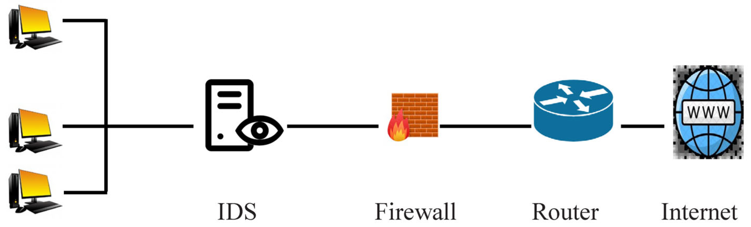
Figure 2 depicts the network-based Intrusion Detection System following the rephrased active voice.

2. Related Works

In the comparison, the Generative Adversarial Network (GAN) algorithm outperformed the Artificial Neural Network (ANN), Multilayer Perceptron (MLP), K-Nearest Neighbor (KNN), Decision Tree (DT), Convolutional Neural Networks (CNNs), and Auto Encoder techniques. The Generative Adversarial Network (GAN) method previously achieved a 99.34 percent classification accuracy [10]. The research described in [11] used machine learning and data mining techniques to combat network intrusion. The focus was on improving the intrusion detection rate while reducing false alarms. The paper [11] explores rule learning using RIPPER on imbalanced intrusion datasets and proposes a combination of oversampling, under-sampling, and clustering-based approaches to address the data imbalance. The evaluation of real-world intrusion datasets showed that oversampling through synthetic generation outperforms replication, and the clustering-based approach enhanced intrusion detection beyond synthetic generation alone. As the aforementioned article describes, an Intrusion Detection System (IDS) is a network security technology that monitors hostile activity on computers or networks. However, due to the dynamic and complicated nature of cyberattacks, typical IDS techniques require assistance. As a result, Ref. [11] proposes that effective adaptive methods, including machine learning approaches, can result in reduced false alarms, increased detection rates, and affordable computational costs.

The performances of several methods based on conventional Artificial Intelligence (AI) and Computational Intelligence (CI) have previously been compared and reviewed. This has highlighted how the characteristics of CI techniques can be utilized to build effective IDSs [12].

Pervez, M.S., Farid, D.M. [13] reviewed the classification accuracy of various classifiers using different dimensional features. Liu, H. and Hussain, F. [14] proposed a novel approach that combines classification and techniques for the multiclass NSL-KDD Cup99 dataset. The proposed method utilizes Support Vector Machines (SVMs). Shapoorifard, H., Shamsinejad, P. [14] researched novel technologies to enhance the classification accuracy of Center and Nearest Neighbors (CANN) Intrusion Detection Systems. They evaluated the effectiveness of these technologies using the NSLKDD Cup99 dataset.

In ref. [15], the authors discuss the hazards of hostile assaults on the network due to widespread internet use. They emphasize how crucial effective Intrusion Detection Systems are for categorizing and foreseeing cyberattacks. According to [15], a hybrid model that combines a firefly-based machine learning technique with Principal Component Analysis (PCA) can be used to categorize Intrusion Detection System (IDS) datasets. The XGBoost method uses hybrid PCA–firefly for dimensionality reduction in the model and classification and alters the dataset with One-Hot encoding. The proposed model outperformed the most advanced machine learning methods based on the experimental data.

In ref. [16], the authors selected 55 features out of an initial 80, achieving a final accuracy of 95% by using the Deep Neural Network (DNN) and Binary Particle Swarm Optimization (BPSO) approaches and the classification method.

Lava, A., Savant, P. [17] describe a machine learning-based NIDS model for binary classification of the CSECIC-IDS2018 using the AWS dataset. The abuse detection techniques of logistic regression, random forest, and gradient boosting were all implemented. However, we discovered that gradient boosting outperformed the others. The model’s performance on the test dataset demonstrated its generalizability. Created using gradient boosting, the estimator exhibited a recall and precision of 0.98, making it suitable for practical applications. Applying synthetic minority oversampling to categorize minority classes of assaults more accurately in the future and running more tests on new data from various network environments using the CIC-IDS-2017 dataset are two potential enhancements [17].

In a survey, Kwon, D., Kim, H. et al. [18] investigated deep learning approaches in anomaly-based network intrusion detection. The authors presented a comprehensive outline of anomaly detection techniques, encompassing data reduction, dimension reduction, classification, and deep learning approaches. The survey [18] covered prior research on deep learning techniques for network anomaly detection, emphasizing its advantages and possible drawbacks. Additionally, the authors conducted local experiments and discovered encouraging outcomes when analyzing network traffic using a Fully Convolutional Network (FCN) model. Regarding anomaly detection accuracy, the FCN model outperformed traditional machine learning methods like Support Vector Machine (SVM), Random Forest, and Adaboosting. Intrusion Detection Systems, or IDSs, are crucial for computer security because they identify and halt malicious activity in computer networks.

An enhanced IDS that incorporates two-level classifier ensembles and hybrid feature selection is presented in [19]. The hybrid feature selection method uses the Ant Colony Algorithm, Genetic Algorithm, and Particle Swarm Optimization to minimize the feature size of training datasets (UNSW-NB15 and NSL-KDD). They selected features based on how well a Reduced Error Pruning Tree (REPT) classifier performs in classification. REPT is a two-level classifier ensemble that uses bagging meta-learners and rotation forests. The suggested classifier outperformed recently developed classification algorithms, displaying 85.8% accuracy, 86.8% sensitivity, and an 88.0% detection rate on the NSL-KDD dataset. The UNSW-NB15 dataset showed similar improvements. We further validated the experimental results using a two-step statistical significance test, which improved the usefulness of the suggested classifier in the ongoing IDS study.

The intelligent Intrusion Detection System described in [20] dramatically enhanced detection performance using an Artificial Neural Network (ANN) model. The ANN-based classifier showed 100% sensitivity on the test dataset with high precision in minimizing false positives. The authors [20] integrated an offline method with a current dataset to find patterns in web application attacks. Aims for future studies include applying this method to the most recent dataset from the Canadian Institute for Cybersecurity (CI-RA-CIC-DoHBrw-2020), implementing further real-time optimizations, and integrating it into an online Intrusion Detection System for testing with real-time network data.

The performance of machine learning techniques, such as Board Learning System (BLS), Radial Basis Function Network (RBF-BLS), and BLS with cascades of mapped features and enhancement nodes, was assessed. The scrutiny encompassed an in-depth examination of malicious intrusions and anomalies within communication networks. The studies used subsets of the CICIDS 2017 and CSECIC-IDS 2018 datasets containing DoS attacks. Even with fewer pertinent features, the models’ performances were comparable, as shown in [21]. Most models attained accuracies and F-Scores above 90%, even though more significant numbers of mapped features and enhancement nodes increased memory needs and training times. Compared to non-incremental BLS, incremental BLS had a noticeably reduced training time [21].

In [22], a thorough examination of deep learning techniques for intrusion detection was performed. Seven deep learning models—deep neural networks, convolutional neural networks, restricted Boltzmann machines, recurrent neural networks, deep belief networks, deep Boltzmann machines, and deep Auto Encoders—were evaluated for their binary and multiclass classification performances. The CSE-CIC-IDS 2018 and Tensorflow systems were used as the software library and benchmark dataset, respectively.

The evaluation relied upon critical performance indicators such as accuracy, detection, and false alarm rates [23], comprehensively assessing the system’s capabilities. The outcomes indicate that deep neural networks can detect intrusion in software-defined networks. This approach demonstrated good results on the latest network attack datasets, leveraging the specific characteristics of Software Defined Network (SDN), such as using the network as a sensor through OpenFlow. Utilizing machine learning techniques for traffic analysis in SDN can enhance the efficiency of network resource allocation. Future work will focus on further analysis of intrusion detection methods and developing an Intrusion Detection System (IDS) using machine learning methods [23].

In ref. [24], the authors developed an ID system using Spark. Moreover, the Convolutional Autoencoder (Conv-AE) deep learning approach efficiently learned feature representations from the CICIDS 2018 dataset. The proposed system outperformed traditional security approaches regarding attack detection rate, accuracy, and computation complexity. The research suggests [24] that this approach can be extended to other fields, such as real-time anomaly and network misuse detection, using deep learning as an attribute extraction tool.

In order to detect network threats, Ref. [25] suggested the use of three models (LSTM, Apache et al., and Random Forest) that use the random forest approach to reduce dimensionality. The application of oversampling and undersampling strategies stemmed from the dataset’s inherent imbalance. Apache Spark had the fastest training time across all classes compared to DL models. Future work could involve semisupervised learning and expand beyond signature-based Intrusion Detection Systems.

One study reported that the Long Short-Term Memory (LSTM) algorithm attained a maximum accuracy of 99 percent [26].

Modern cybersecurity requires detecting network breaches, and researchers have used machine learning to detect and stop attacks [27]. In network intrusion detection, more attention has recently been drawn to deep learning. However, present evaluations utilizing outdated datasets must address class imbalance issues, which may produce biased conclusions. In [27], the authors offer insightful information by resolving this imbalance and assessing Deep Neural Networks, Convolutional Neural Networks, and Long Short-Term Memory Networks on a balanced dataset. With the lowest False Alarm Rate (2.615%), F1-Score (83.799%), and excellent accuracy (84.312%), the Deep Neural Network demonstrated the most outstanding performance [27].

Network Intrusion Detection Systems rely on efficient algorithms and methods for real-time assault detection [28]. One study proposed a preprocessing technique that significantly reduced traffic analysis time and achieved high success rates. Experimental results showed that the ExtraTree algorithm obtained a 99.0% detection rate for binary classification and an 82.96% reduction in processing time per sample. With a 64.43% decrease in processing time per sample, the Random Forest method produced a 98.5% identification rate in the multiclass detection scenario. These results indicate similar categorization rates to previous research, albeit with much shorter test durations [28].

Excellent accuracies have been obtained in the mentioned studies. However, the main problem of these studies is that, to obtain excellent accuracies for detecting intrusion in computer networks, a large number of features are used, or if the number of features is small, excellent accuracies have yet to be obtained. The other issue is that in cases where good accuracies have been obtained, either the model-building times—which is an essential criterion in the case of intrusion detection—have yet to be mentioned or the model-building times are too high. Moreover, in this research, both criteria, i.e., intrusion detection with very high accuracy with the least number of features and building the model in the shortest possible time, have been examined. We demonstrated excellent accuracies of approximately 99% with both the least number of features and the least time taken to build the model.

3. Theoretical Background

Everyday events rely on monitored input data. The IDS generates accurate alarms as informative output, reflecting the events under surveillance. Its primary function involves analyzing the input data [29,30].

Alerts are generated and streamed to show whether intrusions are present. The categorization of every input data stream unit as either standard or invasive represents a random variable X. A low value (X = 0) indicates regular and non-intrusive traffic. In contrast, a high value (X = 1) indicates an incursion. Similarly, a random variable Y represents the output information from the IDS, with Y = 1 denoting an intrusion warning and Y = 0 denoting no signal [29,30].

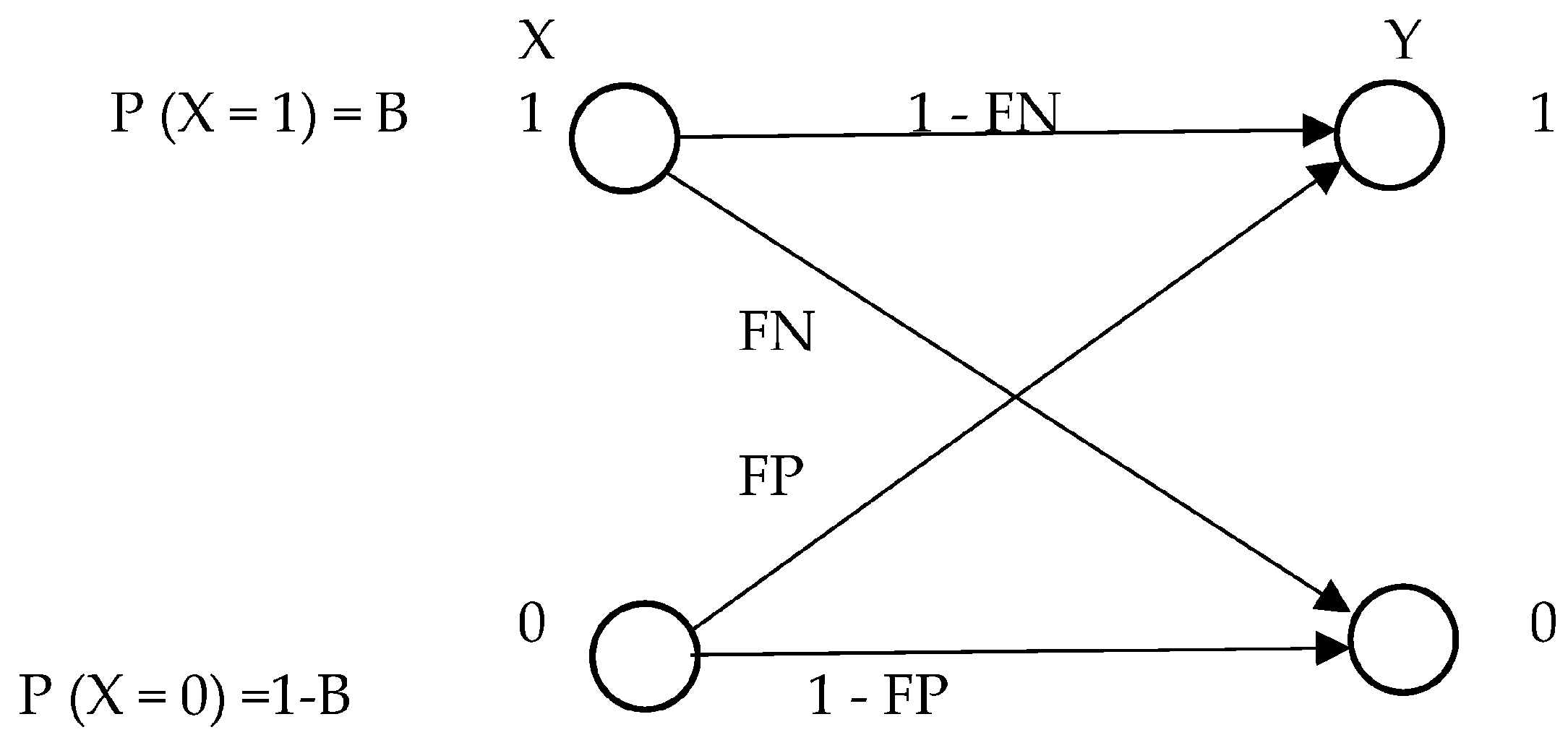
Intrusion detection can be patterned using a binary symmetric channel, which incorporates information theory and provides a framework for understanding intrusion detection. The base rate, or prior probability (B), denotes the chance of intrusions in the input data that the Intrusion Detection System (IDS) has detected. Denoted as γ, the false negative rate (FN) indicates the likelihood of an intrusion event being categorized as usual (p(Y = 0 | X = 1)); on the other hand, the false positive rate (FP), represented by α, is the likelihood that a typical event will mistakenly be classified as an incursion (p(Y = 1 | X = 0)). In this instance, X stands for the IDS input’s random variable. For IDS output, Y stands for the random variable. It is, therefore, feasible to characterize intrusion detection capabilities accurately [29,30]. Figure 3 illustrates the application of Binary Symmetry in an Intrusion Detection Model.

We suggest a new metric called Intrusion Detection Capability, or CID. It is the simple ratio of the input’s entropy to the mutual information between the IDS’s input and output.

Entropy and mutual information are related—H(X) = I(X; Y) + H(XjY), for instance.

The entropy H(Y) is significantly greater than H(X) on the right. This represents a plausible IDS scenario in which H(X) is almost zero due to a minimal base rate that is almost zero. However, the IDS may generate a lot of false positives. Therefore, H(Y) may be greater than H(X).

Let X and Y be the random variables representing the IDS input and output, respectively. The definition of Intrusion Detection Capability is Equation (1):

$${\mathrm{C}}_{\mathrm{I}\mathrm{D}}=\frac{\mathrm{I} \left(\mathrm{X} ; \mathrm{Y}\right)}{\mathrm{H} \left( \mathrm{X} \right)}$$

(1)

Equation (2) allows us to articulate the idea of $C_{ID}$ (Conditional Intrusion Detection) based on our knowledge of mutual information and information theory:

$${\mathrm{C}}_{\mathrm{I}\mathrm{D}}=\frac{\mathrm{H} \left(\mathrm{X}\right)-\mathrm{H} \left(\mathrm{X} \mathsf{l} \mathrm{Y}\right)}{\mathrm{H} \left(\mathrm{X}\right)}$$

(2)

When considering this, we quantify the decrease in ambiguity about the Intrusion Detection System input using mutual information.

Equation (2) illustrates that the $C_{ID}$ represents the proportion of uncertainty reduction in the Intrusion Detection System input due to the Intrusion Detection System output. Practically speaking, the $C_{ID}$ value is between 0 and 1. An increased $C_{ID}$ value indicates an improved ability of the Intrusion Detection System to classify events [29,30].

The mutual information H(X) formula (Equation (3)) defines the mutual information of an event [14].

H (X|Y) is expressed in Equation (4):

$$\mathrm{H}\left(\mathrm{X}\right)=-{\sum }_{\mathrm{X}}^{ } \mathrm{p}\left(\mathrm{x}\right)\log \mathrm{p}\left(\mathrm{x}\right)=-\mathrm{B}\log \mathrm{B}-\left(1-\mathrm{B}\right)\log \left(1-\mathrm{B}\right)$$

(3)

$$\mathrm{H}\left(\mathrm{X}\mathsf{l}\mathrm{Y}\right)=\frac{-{\sum }_x^{ }{\sum }_y^{ }p\left(x\right)p\left(y\mathsf{l}\mathrm{x}\right)\mathrm{l}\mathrm{o}\mathrm{g}\left[\mathrm{p}\left(\mathrm{x}\right)\mathrm{p}\left(\mathrm{y}\mathsf{l}\mathrm{x}\right)\right]}{p\left(y\right)}=-\mathrm{B} (1-\mathsf{\gamma }) \log \mathrm{PPV}-\mathrm{B}\mathsf{\gamma }$$

(4)

log (1 − NPV) − (1 − B)(1 − α) log NPV − (1 − B) α log (1 − PPV)

Equation (5) is obtained by substituting the equations and is the expression for $C_{ID}$:

$${\mathrm{C}}_{\mathrm{I}\mathrm{D}}=\frac{-\mathrm{B}\mathrm{l}\mathrm{o}\mathrm{g}\mathrm{B}-\left(1-\mathrm{B}\right)\log \left(1-\mathrm{B}\right)}{\begin{array}{c}-B\left(1-\mathsf{\gamma }\right)\log PPV-B\gamma \log \left(1-\mathrm{N}\mathrm{P}\mathrm{V}\right)-\left(1-\mathrm{B}\right)\left(1-\mathsf{\alpha }\right) log NPV-\left(1-\mathrm{B}\right)\alpha \log \left(1-\mathrm{P}\mathrm{P}\mathrm{V}\right)\\ \end{array}}$$

(5)

The Intrusion Detection Capability (C_ID) formula, which gauges how well a system detects intrusions, is shown in Equation (5). This equation defines several parameters: the symbols for base rate (B), false negative (FN) rate (γ), false positive (FP) rate (α), positive predictive value (PPV), and negative predictive value (NPV), which are as follows [1]:

The base rate (B) characterizes the Intrusion Detection System’s (IDS) operational environment. A value of B = 0 or B = 1 indicates that the input solely consists of regular or intrusive events, respectively. On the other hand, figuring out or managing the base rate in practice could be difficult for practitioners. This challenge stems from the fact that they frequently utilize base rate as an operational metric to assess the IDS environment. References [30,31] provide a detailed discussion on estimating base rate B and prior probabilities.

The probability that an alert would sound without an intrusion is an Intrusion Detection System’s false positive (FP) rate (IDS).

The false negative (FN) rate represents the likelihood that the Intrusion Detection System fails to raise the alarm when an intrusion occurs [30,31].

When the IDS raises an alarm, the positive predictive value (PPV) measures the likelihood that an intrusion is present. It shows the percentage of IDS alarms that are related to real incursions. The PPV can be expressed mathematically as Equation (6):

$$\mathrm{P}\mathrm{P}\mathrm{V}=\frac{\mathrm{B}(1-\mathsf{\gamma })}{\mathrm{B}\left(1-\mathsf{\gamma }\right)+(1-\mathrm{B})\mathsf{\alpha }}$$

(6)

A negative predictive value (NPV) shows the probability of no incursion when the Intrusion Detection System (IDS) does not sound an alarm. Put otherwise, it quantifies the probability that the absence of Intrusion Detection System (IDS) alerts accurately implies the absence of invasions. Equation (7) provides the mathematical expression for NPV [32,33,34,35]:

$$\mathrm{N}\mathrm{P}\mathrm{V}=\frac{(1-\mathrm{B})(1-\mathsf{\alpha })}{\left(1-\mathrm{B}\right)\left(1-\mathsf{\alpha }\right)+\mathrm{B}\mathsf{\gamma }}$$

(7)

4. Methodology

4.1. Data Cleaning

We implemented several steps to preprocess the CSE-CIC-IDS2018 dataset during the data-cleansing stage. Firstly, we removed specific fields that were deemed redundant or irrelevant. We eliminated the protocol column since each destination port’s Dst_Port (Destination Port) field previously provided equivalent protocol values.

Additionally, we removed the Timestamp parameter to ensure unbiased learning and avoid time-based distinctions, allowing learners to differentiate between high-volume and covert attacks accurately. Removing the timestamp field also facilitated convenient dataset combinations or divisions for our experimental frameworks.

Furthermore, we identified and removed 59 record header row duplicates by filtering the data using an empty list of acceptable label values. Among the downloaded files, ‘Tuesday-20-02-2018_TrafficForML_CICFlowMeter.csv’ (https://www.kaggle.com/datasets/solarmainframe/ids-intrusion-csv accessed on 20 October 2023) stood out as distinct from the other nine files. From this file, we excluded four additional fields: FlowID, Source Internet Protocol (SrcIP), Source Port (SrcPort), and Destination Internet Protocol (DstIP). Moreover, we eliminated all occurrences of negative values in the Fwd_Header_Length, Flow_Duration, and Flow-IAT-Min fields, as these values were consistent with their respective fields. Negative values in the fwd_Header_Length field that correspond with extreme values in other fields can distort outlier-prone statistics. Additionally, we removed records where the values in eight specific fields were zero.

Table 1. List of fields removed prior to feature selection.

No	Feature
1	Bwd_Avg_Bulk_Rate
2	Fwd_Avg_Bytes_Bulk
3	Bwd_Avg_Packets_Bulk
4	Fwd_Avg_Bulk_Rate
5	Bwd_PSH_Flags
6	Fwd_Avg_Packets_Bulk
7	Bwd_Avg_Bytes_Bulk
8	Bwd_URG_Flags

provides the complete list of removed fields before feature selection.

We did not include the Init_Win_bytes_backward and Init_Win_bytes_forward fields due to approximately 50 percent having negative numbers corresponding to these variables.

Similarly, we chose not to utilize the Flow_Duration fields because some values were unreasonably low or zero. Less than 0.6 percent of entries in the Flow Packets/s and Flow Bytes/s columns included “NaN” or “Infinity” values. We eliminated cases when the flow bytes or packets per second had such values.

After completing the data cleaning stage and before feature selection, we applied an unsupervised approach and the discretize filter method to filter our data; this involved using an instance filter called “Discrete” to convert various numerical properties of the dataset into nominal attributes.

The CSE-CIC-IDS2018 dataset consists of 10 files collected over consecutive days. The resulting dataset contained 16,232,943 records and 80 features upon merging these files. Following the data cleaning process, 16,137,168 records and 67 features remained in the dataset. For the data filtering step, we utilized this enhanced dataset. Of the entire amount of records collected (16,137,168), we reserved 3,227,433 records (20 percent) for system testing and assessment, and we assigned 12,909,735 records (80%) for system training.

Table 2. Quantity and percentage of each traffic class before and after data cleaning.

Traffic Class	Before Data Cleaning	Percentage before Data Cleaning	After Data Cleaning	Percentage after Data Cleaning
Benign	13,484,708	83.070%	13,390,234	82.978%
DDoS	1,263,933	7.787%	1,263,933	7.832%
Bot	286,191	1.76%	286,191	1.773%
Brute Force	380,949	2.347%	380,943	2.361%
Infiltration	161,934	0.998%	160,639	0.995%
Dos	654,300	4.032%	654,300	4.055%
Web Attack	928	0.0055%	928	0.006%
Total	16,232,943		16,137,168

provides a visual representation of the quantity and percentage of each traffic type before and after the completion of the data-cleaning process.

4.2. Data Filtering

In data mining, ensuring data quality for subsequent mining stages is of utmost importance. Data preprocessing plays a vital role in accomplishing this objective. Its primary aim is to improve the quality of mining outcomes by cleaning the collected data, encompassing activities such as data transformation and dimensionality reduction. In discretization, one transforms continuous or numerical variables into discrete or nominal attributes by dividing them into a finite number of intervals [36,37].

Among the top ten data mining algorithms are machine learning approaches like naive Bayes, Apriori, decision trees, and leveraged data discretization [38,39,40]. By employing data discretization, these techniques construct more effective and efficient models. Moreover, transforming continuous features into discrete counterparts provides a representation that aligns with knowledge-level understanding, making them easier to comprehend, utilize, and explain than continuous attributes [38].

In a comparison study, Garcia et al. [40] examined the classification performance of 30 discretized algorithms utilizing a slow, rule-based decision tree and Bayesian learning techniques. Their work provides information on discretizations appropriate for a particular classifier type, those that work with all classifier types, and those that strike a decent balance between the number of intervals generated and the precision of classification. Data discretization divides the range into short intervals showing strong class coherence to determine a set of cut points for continuous features.

Additionally, discretization techniques should reduce the number of intervals while maintaining a high degree of mutual dependency between classes and attributes. Because of this, we partitioned continuous features into k intervals, or portions, with a maximum of k − 1 cut points. The trade-off between the arity (number of intervals) and its effect on accuracy must be considered [38].

The subsequent section summarizes the data discretization process applied to a dataset containing N examples and C target classes. We apply an algorithm for discretization to transform the continuous attribute A into m discrete intervals represented by D = {[d0, d1], [d1, d2],…, [dm − 1, dm]}, where d0 is the minimum value, dm is the maximum value, and di < di + 1 for i = 0, 1,…, m − 1. The resulting discrete representation D is a discretization scheme for attribute A, and P = {d1, d2,…, dm − 1} represents attribute A’s set of cut points [21]. Sorting the continuous feature values, identifying and assessing cut issues for splitting or merging intervals, dividing or merging constant intervals depending on particular criteria, and stopping at a specific point are the four general processes of the discretization process [38].

Discretization algorithms can be categorized based on different characteristics [38,39,41], as described below:

Dynamic vs. Static: Static discretization is performed before and does not depend on the learning algorithm and the learning task; while creating a model, dynamic discretization occurs. The most commonly used discretizations are static, whereas the discretized ID3 decision tree is an example of a dynamic discretization.

Comparing univariate and multivariate discretization, the former examines a single continuous feature, while the latter considers several features simultaneously.

Supervised versus unsupervised discretization methods differ in their approach to determining appropriate intervals during the discretization process. Supervised methods utilize class information to guide the selection of intervals, considering the class membership of the data. On the other hand, unsupervised methods do not consider class membership when discretizing the data. It is important to remember that the majority of discretization methods require supervision.

Splitting vs. merging: while merging methods begin with a pre-defined partition and remove a potential cut-point to combine nearby intervals, splitting methods select a cut-point from among all available boundary points to divide the domain into two intervals.

Local vs. global: Local discretization bases its partition decisions solely on local data, whereas global discretization handles the discretization of every numeric property during preprocessing. Global discretization techniques typically perform better than local ones.

Incremental vs. Direct: Since direct approaches divide the range into k intervals concurrently, they require an extra criterion to find k. Conversely, incremental approaches begin with a straightforward discretization and proceed through an improvement process; however, they need an extra criterion to decide when to end the process. We used an unsupervised strategy to filter the data after the data-cleaning stage before selecting features. In particular, we applied a discretized filter approach called “Discrete”—an instance filter. The many numerical properties of the dataset were converted into notional qualities using this filter.

4.3. The Selection of Features

An essential component of machine learning is feature selection, which directly impacts classification performance. A well-chosen feature set leads to higher accuracy in classification tasks. This study employs four feature selection approaches: the Ant, Bee, Bat, and Wolf algorithms, each selecting various features.

After the data cleaning stage, our dataset consisted of 67 features. We employed four algorithms (Ant et al.).

Table 3. Features selected by applying the bee algorithm.

No	Feature
1	Dst Port
2	Fwd IAT Min
3	Bwd Pkts/s
4	Fwd Seg Size Min
5	Fwd Act Data Pkts

,

Table 4. Features delected by applying the Flower Pollination Algorithm.

No	Feature
1	Dst Port
2	Fwd Pkt Len Min
3	Flow Pkts/s
4	Bwd Pkts/s
5	Fwd IAT Min
6	ECE Flag Cnt
7	ACK Flag Cnt
8	Fwd Seg Size Min
9	Fwd Act Data Pkts

,

Table 5. Features chosen using an Ant Colony Optimization algorithm.

No	Feature
1	Dst Port
2	Flow Pkts/s
3	Fwd IAT Max
4	Flow, IAT Min,
5	Fwd Pkts/s
6	Fwd Header Len
7	Bwd Pkts/s
8	RST Flag Cnt
9	Fwd Seg Siz Min
10	Idle Std

and Table 6 show the outcomes of using four distinct algorithms.

4.3.1. ABC, or Artificial Bee Colony (ABC)

The Artificial Bee Colony (ABC) algorithm takes cues from honey bee activities. Finding the best answers to various issues is made possible by a swarm intelligence system known as colonies [42]. This represents a potential food supply by each point in the search space of the ABC algorithm, which depicts the surroundings of a colony of honey bees. Each food source has a different amount of nectar, and those indicate the fitness value of the food supply. Researchers use three different types of bees in the ABC algorithm: scout, employed, and observation bees [42,43].

The algorithm only plans to provide a working bee with food. Worker bees figure out how much nectar there is. There are the same number of workers in the colony and observers of artificial bees. The task of collecting high-quality data and forwarding it to observer bees falls to employed bees.

Consequently, nectar-rich food sources will be directed toward observers among the bee population. We continued these steps until we obtained the limit value. Researchers have developed numerous ABC algorithms in the literature [44] for various purposes. Researchers have created numerous enhanced ABC variations to address global optimization issues [45].

To create test cases, for example, two novel combinatorial ABC algorithms with many requirements have been devised [46]. These algorithms improve both intensification and variety in the bee population by optimizing coverage criteria.

There are five primary phases to the ABC algorithm:

First Step: Based on the amount of food sources indicated by SN, the initialization randomly creates the initial food sources. Two times SN (SN employed bees + SN onlooker bees) is the colony size NP. We generate food sources between the variables’ top and lower boundaries. Equation (8) generates the food source positions during the startup stage:

X_ij = X_minj + rand(0,1)(X_maxj − X_minj)

(8)

In dimension j, where j = 1, 2, 3,…, D, Xminj, and Xmaxj represent the lower and upper bounds. SN defines the number of worker or observer bees. For every solution, we construct a D-dimensional vector xi (i = 1, 2,…, SN), where D is the quantity of optimization factors.

Following the initialization stage, we repeat cycles with the populations of the scout, employed, and onlooker bees C = 1, 2…, MCN used in the solution search strategies. MCN is the maximum count of iterations.

Second step: Evaluate the food sources’ fitness value (i.e., nectar amount). We use Equation (9) to compute the attributes of every food source individually:

$${fit}_i=\left\{\begin{array}{c}\frac{1}{1+f_i}, if(f_i\ge 0) \\ 1+abs\left(f_i\right), otherwise\end{array}\right.$$

(9)

where fit_i is the value of the specific objective function and fi is the fitness of the ith food source.

Third Step: After initialization and fitness calculations, the employed bees, following the bee method, explore new food sources with better nectar. Every worker bee updates the locations of their relevant food sources. This way, we create a new food source position υij:

$${\upsilon }_{ij }=X_{ij}+{\varphi }_{ij}(X_{ij} {-X}_{kj})$$

(10)

The letters j ϵ {1, 2,…, d} and k ϵ {1, 2,…, SN} represent the randomly selected index values. The uniform random number ʝij, in this instance, is located in the interval [−1, 1]. In dimension j, the reference and randomly chosen food sources are at Xij and Xkj, respectively.

Equation (9), once we have established υij, is used to calculate its fitness value. An employed bee stores the position of the new food source when its fitness exceeds that of the previous one.

Fourth step: The onlooker bee method: Each chooses a food source based on the fitness values determined in Step 3. High-fitness food sources are more likely to be chosen than others in this selection mechanism [42]. We compute the probability as follows:

$${ p}_i=\frac{{fit}_i}{{\sum }_{k=1}^{SN}{fit}_k}$$

(11)

Upon determining the probability value pi, each food source produces a random integer known as its fitness value or fit_i. If there is a higher chance of locating the food source than this random number, the spectator bee is given a current food source for the searching–exploiting process. Bystander bees then identify the precise food sources. Similar to the previous bee stage, we evaluated the new technique.

Fifth step: Process of the scout bee: The ABC algorithm states that the number of food sources (i.e., solutions) and trial counts determine the incidence of scout bees. A deployed bee’s trial counter value will depart from the food source if it exceeds the upper limit. After that, the working bee changes into a scout bee. The scout bee looks for new food sources.

Using a simulated bee colony, we selected the characteristics in Table 3.

4.3.2. The Algorithm for Flower Pollination (FPA)

The FPA is a population-based global optimization algorithm.

Yang et al. summarized the features of the Flower Pollination Algorithm procedure into the following four perfect guidelines [47].

Rule 1: Cross-pollination by pollinators, like birds, represents a global pollination stage. Pollinators behave like light birds;

Rule 2: the local pollination process starts with self-pollination on nearby flowers;

Rule 3: the reproduction rate, or floral constancy, is a straight ratio comparable to the two flowers under consideration;

Rule 4: a switch probability implements local and global pollination.

According to the previously mentioned principles, the FPA has a local and a global pollination operator. Every pollen item in the FPA is considered a solution SX_i; the initialization of solutions within the feasible search space involves the utilization of random vectors. Presented below is the original formula [48]:

$${ SX}_i=\mathrm{L}\mathrm{o}\mathrm{w}\mathrm{e}\mathrm{r}+R_{\upsilon }\left(\mathrm{U}\mathrm{p}\mathrm{p}\mathrm{e}\mathrm{r}-\mathrm{L}\mathrm{o}\mathrm{w}\mathrm{e}\mathrm{r}\right)$$

(12)

where $R_{\upsilon }$ is a D-dimensional random vector in [0, 1] D; the bottom limit of the search space is bottom = [l1,…, ld,…, lD], and the upper limit is Upper = [u1,…, ud,…, uD]. Where i ∈ {1,…, NP}, NP is the population size. Pollinators, like birds, have a comparatively wide range of motion and can transport pollen across great distances as part of the global pollination process. Thus, the following is how Rules 1 and 3 are formulated [48]:

$${ SX}_i^{t+1}={\mathrm{S}\mathrm{X}}_i^t+\mathsf{\gamma }\mathrm{L}\left(\mathsf{\lambda }\right)\left(gbest-{SX}_i^t\right)$$

(13)

By using the levies distribution denoted by (λ) in (13), we may numerically simulate the flight behavior of birds. Furthermore, (λ) can be regarded as a variable step factor for pollination intensity measurement. As a step factor, γ is the solution i at iteration t, and abest is the current global best solution. When L > 0, the levy distribution can be explained as follows [48]:

$$L~ \frac{\lambda Г\left(\lambda \right)\sin \left(\pi \lambda /2\right)}{\pi }\frac{1}{s^{1+\lambda }}, s\gg s_0>0 , s_0=0.1,$$

(14)

Using the two Gaussian distributions, U and V, and the standard gamma function, Г (λ), whose λ = 1.5 [48], we compute s:

$$s=\frac{U}{{\left|V\right|}^{1/\lambda }} , U ~ N \left(0,{\delta }^2\right), V ~ N \left(\mathrm{0,1}\right)$$

(15)

$${ \delta }^2={\left\{\frac{Г(1+\lambda )}{\lambda Г[\left(1+\lambda \right)/2 ]} . \frac{sin(\pi \lambda /2)}{2^{(\lambda -1)/2}} \right\}}^{1/\lambda }$$

The conventional normal distribution is shown by (0, 1), and the normal distribution with mean value 0 and variance δ2 is denoted by (0, δ2). Local pollination disperses pollen to a nearby neighbor if used in pollination activities. We can create the model as follows [48], using Rules 2 and 3:

$${ SX}_i^{t+1}={SX}_i^t+\xi \left({SX}_j^t-{SX}_k^t\right)$$

(16)

Here, j and k ϵ {1, …, NP} and ξ is a random vector in [0, 1] D of dimension D, and SXj and SXk are the pollen that has been chosen at random from different flowers on the same plant. Moreover, based on Rule 4, the randomness of the two pollination acts is determined by a probability p. In contrast, the opposite is true if a random value rand in [0, 1] is mi-nor; otherwise, p. Figure 4 displays the FPA flowchart [48].

Table 4 shows the features selected using a Flower Pollination Algorithm.

4.3.3. Ant Colony Techniques for Optimization (ACO)

Dorigo and colleagues introduced the Ant System (AS) algorithm in the early 1990s as a cutting-edge meta-heuristic technique for resolving combinatorial optimization issues that drew inspiration from nature. The first problem to be solved by the algorithm was the traveling salesperson problem. Recently, this has been improved and modified to enhance its usefulness and apply it to other optimization problems. Ant Colony System (ACS), AS-rank, MAX-MIN, and AS are the upgraded versions of AS [49].

Ant Colony Optimization mimics the cooperative and adaptive mechanisms of natural ant behavior on an individual level. Real ants’ foraging habits inspire ACO [49]. We based our computational paradigm for the ACO algorithm on actual ant colonies and their functioning. Our goal was to involve as many constructive computational ants as possible. Each ant follows the generated solution, which relies on its dynamic memory structure recording outcomes from past trials.

Ethologists’ findings derived the paradigm regarding the pheromone trail system ants employ to communicate information regarding the most direct paths to food. Upon finding a previously constructed road, an ant can identify it, decide to follow it with a high chance of success, and reinforce the route with its pheromones. A solitary ant, on the other hand, travels around practically at random. What appears is a type of autocatalytic process whereby a track becomes more appealing to ants to follow the more they follow it. As a result, a positive feedback loop defines the process where the likelihood of selecting a path increases in proportion to the number of ants that have already selected that path. The ACO family of algorithms draws inspiration from the abovementioned mechanism [50].

It is also possible to consider a FS period before the training phase. Which traits are more discriminative than others is determined by the FS process. It removes duplicated and unnecessary functionality, improving system performance. Generally speaking, FS is a rare IDS operation. Nonetheless, several researchers have conducted their experiments using various FS techniques. This suggests that FS may raise IDS classification accuracy. The problem in using FS lies in finding a minimal feature subset of size S (S < N) given a feature set of size N while maintaining the prior accuracy. As a result, the FS problem needs a solution path [50,51].

A partial solution, sometimes referred to as a subset, suggests that there is no connection between the elements or characteristics of the solution, and the decision of which element to add to the partial solution after the previous one needs not be influenced [50,51]. FS problems can occasionally have solutions of varying proportions. Redefining the use of the ACO representation graph is the first stage in FS employing ACO.

Using an Ant Colony Optimization algorithm, we selected the attributes shown in Table 5.

4.4. Performance Evaluation

Our study employed a confusion matrix to evaluate a binary classification problem. Such problems often involve classes of interest, including a minority class and its opposite class, commonly called positives and negatives. In this context, several key performance metrics are used [52,53,54]:

True Positive (TP): these correctly anticipated positive results suggest that the actual and forecasted class values are accurate;

True Negative (TN): the fact that neither the actual class value nor the expected class value is positive is one of the precisely predicted negative values;

False Positive (FP): the situation where the expected class is valid but the actual class is false;

False Negative (FN): a situation where the actual class is positive but the projected class is negative;

Accuracy: the percentage of related samples among the retrieved samples is known as accuracy, another name for a positive value:

$$\mathrm{A}\mathrm{c}\mathrm{c}\mathrm{u}\mathrm{r}\mathrm{a}\mathrm{c}\mathrm{c}\mathrm{y}=\frac{\mathrm{T}\mathrm{P}+\mathrm{T}\mathrm{N}}{\mathrm{T}\mathrm{P}+\mathrm{T}\mathrm{N}+\mathrm{F}\mathrm{P}+\mathrm{F}\mathrm{N}}$$

(17)

Precision: precision is the ratio of accurately expected observations to all anticipated positive observations concerning positive observations:

$$\mathrm{P}\mathrm{r}\mathrm{e}\mathrm{c}\mathrm{i}\mathrm{s}\mathrm{i}\mathrm{o}\mathrm{n}=\frac{\mathrm{T}\mathrm{P}}{\mathrm{T}\mathrm{P}+\mathrm{T}\mathrm{N}}$$

(18)

Recall (Sensitivity): the sensitivity is calculated quantitatively by dividing the total number of true positives by the sum of the true and false negatives:

$$\mathrm{R}\mathrm{e}\mathrm{c}\mathrm{a}\mathrm{l}\mathrm{l}=\frac{\mathrm{T}\mathrm{P}}{\mathrm{T}\mathrm{P}+\mathrm{T}\mathrm{N}}$$

(19)

F-measure (F1 score): The F-measure functions as a sort of average between the parameters P (Precision) and R (Recall). P represents the system’s accuracy when compared to the predicted data. We express the number of predicted data to all expected data for prediction as a ratio or r:

$$\mathrm{F}1\mathrm{S}\mathrm{c}\mathrm{o}\mathrm{r}\mathrm{e}=\frac{2\times \mathrm{P}\mathrm{r}\mathrm{e}\mathrm{c}\mathrm{i}\mathrm{s}\mathrm{i}\mathrm{o}\mathrm{n}\times \mathrm{R}\mathrm{e}\mathrm{c}\mathrm{a}\mathrm{l}\mathrm{l}}{\mathrm{P}\mathrm{r}\mathrm{e}\mathrm{c}\mathrm{i}\mathrm{s}\mathrm{i}\mathrm{o}\mathrm{n}+\mathrm{R}\mathrm{e}\mathrm{c}\mathrm{a}\mathrm{l}}$$

(20)

4.5. Time Taken to Build a Model

The algorithm’s duration is required to build the model using the training data.

5. Experimental Design

5.1. Dataset

The Communications Security Establishment (CSE) and the Canadian Institute for Cyber Security (CIC) have jointly developed the CSE-CIC-IDS2018 dataset for attack detection and prevention. This open-source dataset provides traffic patterns and various attacks found in network architecture [52].

There are 80 features in the dataset, including tags, most consisting of data in terms of statistics regarding internet traffic. The CICFlowMeter tool obtains these features by generating information based on network traffic flow. The dataset includes continual characteristics such as labels, timestamps, destination ports, and protocols. It includes six scenarios and fourteen types of assaults, such as botnet, denial of service (DoS), infiltration, Web attack, and DDoS [28,52].

Amazon Web Services (AWSs) offers the CSE-CIC-IDS2018 dataset for download; included are ten CSV files totaling over 16.2 million samples, representing ten recorded network flow days. The CICFlowMeter program extracted more than 80 features to produce the dataset. The CSE-CIC-IDS2018 dataset’s Table 6 [29,54] offers comprehensive details on the different kinds of assaults and safe traffic.

Table 6. Attack types and secure traffic in the dataset CSE-CIC-IDS-2018.

Category	Attack Types
Benign
DDoS	HOIC
	LOIC-HTTP
	LOIC-UDP
Botnet	Bot
Brute Force	FTP
	SSH
Infiltration	Infiltration
Dos	Hulk
	SlowHTTPTest
	GoldenEye
	Slowloris
Web Attack	Web
	XSS
	SQL Injection

Table 6. Attack types and secure traffic in the dataset CSE-CIC-IDS-2018.

Category	Attack Types
Benign
DDoS	HOIC
	LOIC-HTTP
	LOIC-UDP
Botnet	Bot
Brute Force	FTP
	SSH
Infiltration	Infiltration
Dos	Hulk
	SlowHTTPTest
	GoldenEye
	Slowloris
Web Attack	Web
	XSS
	SQL Injection

Table 7. The CSE-CIC-IDS2018 dataset’s record count.

Traffic Class	Record Count	Share (%)
Benign	13,484,708	83.070%
HOIC	686,012	4.226%
LOIC-HTTP	576,191	3.550%
Hulk	461,912	2.846%
Bot	286,191	1.76%
FTP—BruteForce	193,360	1.191%
SSH—BruteForce	187,589	1.156%
Infiltration	161,934	0.998%
SlowHTTPTest	139,890	0.862%
GoldenEye	41,508	0.256%
Slowloris	10,990	0.068%
LOIC-UDP	1730	0.011%
Brute Force—Web	611	0.004%
Brute Force—XXS	230	0.001%
SQL Injection	87	0.0005%

shows the record count and attack percentage of the CSE-CIC-IDS2018 dataset.

There are 16,232,943 records in the CSE-CIC-IDS2018 dataset, with 83.07 percent (or records) consisting of benign traffic, while the remaining records represent malicious activity. This study used 80 percent of the records for training, while the remaining 20 percent was allocated for testing [28,29,52,53,54,55].

5.2. Experimental System Specifications

The experimental design for this study involved implementing the test procedure on a system comprising an AMD Ryzen 7 1800X eight-core processor (Santa Clara, CA, USA) operating at a clock speed of 3.60 GHz, paired with 32 GB of RAM and 128 GB allocated as swap space on the hard disk. The system employed an X64-based processor and ran on Windows 10 Enterprise as the operating system.

6. Results

Utilizing a range of machine learning algorithms, we performed experiments by dividing 80% of the dataset for training the system while allocating the remaining 20% to evaluate its performance. The feature selection techniques included Ant Colony Optimization (ACO) algorithms, the Flower Pollination Algorithm (FPA), and Artificial Bee Colony (ABC). Subsequently, these selected features were tested and evaluated with various machine learning algorithms.

Table 8. Results of different algorithms using features selected by the Ant Colony Optimization (ACO) algorithms.

Algorithm	Time Spent on a Model Build	Accuracy	Precision	Recall	F-Measure
AdaBoostM1	802.44 s	0.862	0.961	0.883	0.920
Bagging	13,969.96 s	0.988	0.996	0.989	0.992
BayesNet	638.07 s	0.965	0.968	0.989	0.979
CDT	1132.89 s	0.987	0.997	0.988	0.993
DTNB	18,733.06 s	0.986	0.996	0.988	0.992
IB1	9 s	0.978	0.986	0.988	0.987
J48	2858.5 s	0.988	0.997	0.988	0.993
KStar	3 s	0.979	0.989	0.987	0.988
Local Knn	324,075 s	0.984	0.993	0.988	0.990
Logistic	35,662 s	0.960	0.981	0.972	0.976
LogitBoost	2752 s	0.982	0.993	0.985	0.989
Multilayer perceptron	17,072 s	0.945	0.968	0.965	0.967
Random Tree	481.24 s	0.983	0.991	0.989	0.990
SMO	48,562	0.891	0.993	0.889	0.938

,

Table 9. Results of different algorithms using features selected by the Flower Pollination Algorithm (FPA).

Algorithm	Time Spent on a Model Build	Accuracy	Precision	Recall	F-Measure
AdaBoostM1	593.74 s	0.862	0.961	0.883	0.920
Bagging	14,089.45 s	0.987	0.996	0.988	0.992
BayesNet	438.8 s	0.978	0.988	0.986	0.987
CDT	991.14 s	0.987	0.997	0.988	0.992
DTNB	9329.23 s	0.986	0.996	0.988	0.992
IB1	7 s	0.978	0.986	0.987	0.987
J48	3003.97 s	0.987	0.997	0.988	0.992
KStar	1 s	0.980	0.990	0.986	0.988
Local Knn	445,905 s	0.983	0.992	0.988	0.990
Logistic	20,578 s	0.946	0.971	0.964	0.968
LogitBoost	2565 s	0.975	0.987	0.983	0.985
Multilayer perceptron	16,290 s	0.956	0.974	0.974	0.974
Random Tree	445.08	0.982	0.991	0.988	0.989
SMO	35,787 s	0.885	0.997	0.880	0.935

and

Table 10. Results of different algorithms using features selected by the Artificial Bee Colony (ABC).

Algorithm	Time Spent on a Model Build	Accuracy	Precision	Recall	F-Measure
AdaBoostM1	430.44 s	0.862	0.961	0.883	0.920
Bagging	6679.11 s	0.966	0.995	0.988	0.992
BayesNet	230.1 s	0.970	0.978	0.985	0.982
CDT	475.84 s	0.986	0.996	0.988	0.992
DTNB	2941.84 s	0.983	0.996	0.984	0.990
IB1	5 s	0.976	0.985	0.986	0.986
J48	1299.04 s	0.986	0.996	0.988	0.992
KStar	2 s	0.977	0.987	0.985	0.986
Local Knn	3,430,073 s	0.982	0.991	0.987	0.989
Logistic	7212.36 s	0.892	0.998	0.887	0.939
LogitBoost	1287.00 s	0.973	0.984	0.985	0.984
Multilayer perceptron	11,008 s	0.926	0.998	0.920	0.957
Random Tree	394.52 s	0.981	0.990	0.987	0.989
SMO	12,496 s	0.890	0.992	0.888	0.938

(values rounded to three decimal places) display the outcomes of these tests.

As can be seen in Table 8, after applying 14 different machine learning algorithms, according to the results obtained, we obtained the best accuracy in intrusion detection by applying the Bagging and J48 machine learning algorithms, of which 98.8% were able to detect different types of cyber threats and distinguish them from regular traffic; furthermore, regarding the shortest time to build the model, the construction time was 3 s using the Ant Colony Optimization feature selection method.

According to the results obtained after selecting features using the Flower Pollination Algorithm by applying different machine learning algorithms, the best result was an accuracy of 98.7 in detecting regular traffic and different cyberattacks. Moreover, the shortest model-building time was one second using the KStar algorithm.

Table 10 shows that the DTNB and J48 machine learning algorithms, combined with the Artificial Bee Colony feature selection approach, yielded the maximum accuracy of 98.6, and that this strategy took the smallest amount of time to develop the model at 2 s.

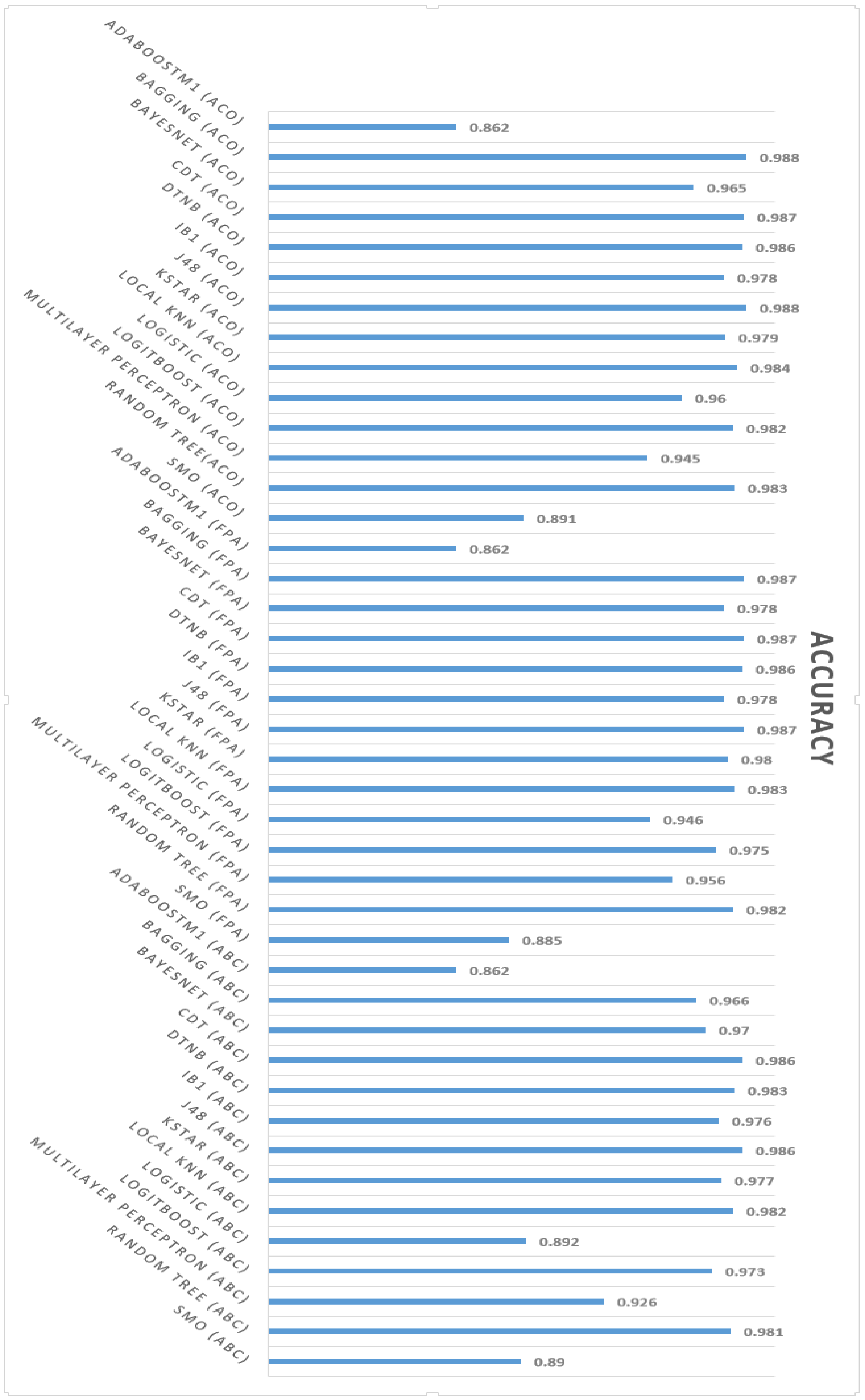
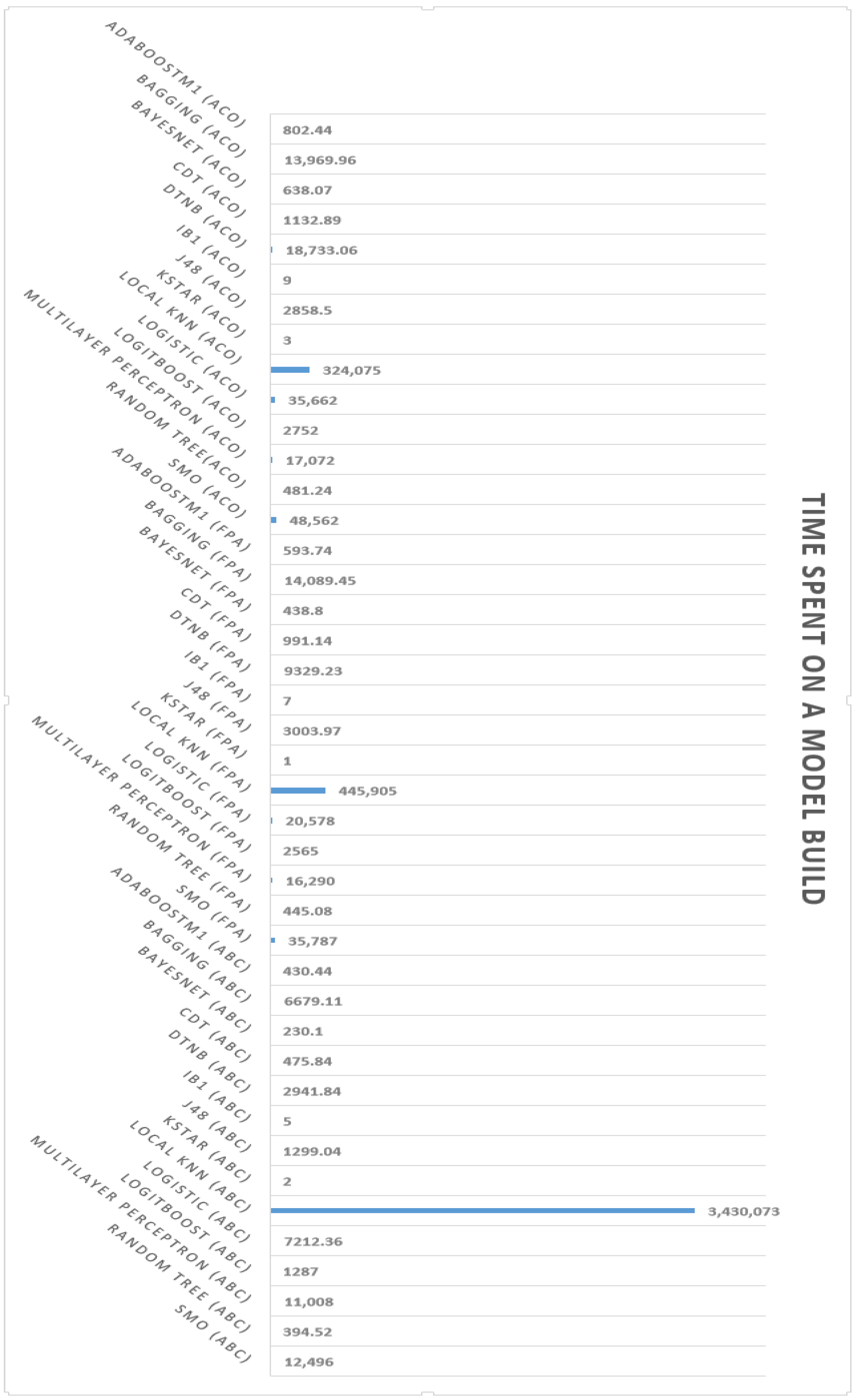
Readers are encouraged to explore the following charts (Figure 5 and Figure 6), portraying the accuracy and time needed for model construction employing various machine learning algorithms alongside diverse feature selection techniques. As shown in Figure 5, the highest accuracy among the three different feature selection methods, including Artificial Bee Colony (ABC), the Flower Pollination Algorithm (FPA), and Ant Colony Optimization (ACO), was that related to Ant Colony Optimization (ACO) with 98.8% using the Bagging and J48 machine learning algorithms. Moreover, the minimum model-building time was related to the Flower Pollination Algorithm (FPA), which was only 1 s using the KStar machine learning algorithm.

7. Discussion

This research introduced novel methodologies by combining various approaches in intrusion detection in computer networks, contributing to advancements in computer science. The initial data cleaning stage was crucial in eliminating disruptive and noisy data that could hinder selecting selection features. After the data cleaning phase, the subsequent step focused on optimizing the selection of valuable features; a filtering method was applied—discretize—to the features obtained, allowing the entry of the most suitable feature set into the selection process. This research employed the Ant Colony Optimization (ACO) algorithms, Flower Pollination Algorithm (FPA), and Artificial Bee Colony (ABC) in conjunction with other feature selection techniques for the first time, generating distinct subsets of features not utilized in similar studies. Remarkably, this study achieved noteworthy accuracy with a minimum number of features. For instance, achieving more than 98% intrusion detection accuracy was possible using only five features, and an impressive accuracy of approximately 99% (equal to 0.988) was achieved using just ten features. These findings represent a significant advancement within the field of Intrusion Detection Systems. Another critical accomplishment of this study is the model-building time facilitated by the employed algorithms. The model-building time was substantially reduced to a minimum of 1 s (With the KStar machine learning algorithm); this emphasizes the efficiency and effectiveness of the algorithms utilized, a crucial aspect often overlooked in previous research endeavors.

In brief, the effectiveness of feature selection and data-cleaning approaches in Intrusion Detection Systems was demonstrated in this study. While drastically cutting down on the time needed to generate the model, using a few features allowed for previously unheard of accuracy levels. Computer science researchers can use these insights to create and enhance Intrusion Detection Systems.

8. Conclusions

This study utilized the CSE-CIC-IDS2018 dataset, comprising 80 features and over 16 million records, to evaluate Intrusion Detection Systems in computer networks, emphasizing its relevance to computer science. This research involved data cleaning and three feature selection approaches. In the initial stage, by utilizing only five features, a remarkable accuracy of 98% in identifying safe traffic and computer attacks was achieved; this demonstrates the effectiveness of feature selection and its impact on accurate intrusion detection. Additionally, this study successfully built a model to detect intrusion in 1 s using only nine features, showcasing efficient performance in time.

Furthermore, in subsequent stages, a model with approximately 99% accuracy was constructed within a reasonable time frame by selecting ten features and employing different feature selection techniques; this highlights the importance of accuracy and time considerations in Intrusion Detection Systems.

Future research should continue refining feature selection methods and exploring data cleaning. Various techniques can be employed to optimize system performance and determine which features influence accurate intrusion detection most. These techniques aim to enhance the overall effectiveness of Intrusion Detection Systems by optimizing system performance and focusing on identifying key features that contribute significantly to accurate detection. One valuable suggestion arising from this study is to consider the priorities of network experts or managers. Depending on their network requirements, they can prioritize either time or accuracy. If time is crucial, they can adopt approaches that prioritize faster detection of attacks. Conversely, investing more time in the detection process can yield higher accuracy if accuracy is paramount. This recommendation gives network experts an essential tip for making informed decisions based on their network’s needs.

Regarding computer networks, especially data centers, using intrusion systems is essential for reducing the damage caused by cyberattacks. One of the most important aspects of preventing intrusions on servers and networked devices is the timely and accurate identification of such intrusions. Intrusion Detection Systems become much more efficient when the number of features required for detection is reduced. This decrease prevents potential slowdowns in intrusion detection operations by reducing excessive memory and CPU consumption and increasing detection speed. For this reason, it is critical to detect assaults on computer networks as soon as possible to prevent serious harm. Furthermore, reaching higher threat detection accuracy gives network specialists more confidence and presents chances for cost savings by switching resources from human involvement to Intrusion Detection Systems’ strong capabilities.