Article

Adaptive Kalman Filter for Real-Time Visual Object Tracking Based on Autocovariance Least Square Estimation

1
Beijing Key Laboratory of Information Service Engineering, Beijing Union University, Beijing 100101, China
2
College of Robotics, Beijing Union University, Beijing 100027, China
3
State Key Lab of Automotive Safety and Energy, School of Vehicle and Mobility, Tsinghua University, Beijing 100084, China
*
Author to whom correspondence should be addressed.
Appl. Sci. 2024, 14(3), 1045; https://doi.org/10.3390/app14031045
Submission received: 30 November 2023 / Revised: 16 January 2024 / Accepted: 24 January 2024 / Published: 25 January 2024
(This article belongs to the Special Issue Autonomous Vehicles and Robotics)

Abstract

:
Real-time visual object tracking (VOT) may suffer from performance degradation and even divergence owing to inaccurate noise statistics typically engendered by non-stationary video sequences or alterations in the tracked object. This paper presents a novel adaptive Kalman filter (AKF) algorithm, termed AKF-ALS, based on the autocovariance least square estimation (ALS) methodology to improve the accuracy and robustness of VOT. The AKF-ALS algorithm involves object detection via an adaptive thresholding-based background subtraction technique and object tracking through real-time state estimation via the Kalman filter (KF) and noise covariance estimation using the ALS method. The proposed algorithm offers a robust and efficient solution to adapting the system model mismatches or invalid offline calibration, significantly improving the state estimation accuracy in VOT. The computation complexity of the AKF-ALS algorithm is derived and a numerical analysis is conducted to show its real-time efficiency. Experimental validations on tracking the centroid of a moving ball subjected to projectile motion, free-fall bouncing motion, and back-and-forth linear motion, reveal that the AKF-ALS algorithm outperforms a standard KF with fixed noise statistics.

1. Introduction

Visual object tracking (VOT) is a fundamental task in computer vision and has extensive applications including autonomous vehicles [1], video surveillance [2], robot vision [3], and human-computer interaction [4]. Specifically, in autonomous vehicle systems and robotics, robust and efficient VOT algorithms that identify and track nearby vehicles and pedestrians are essential for real-time navigation, obstacle avoidance, and environment perception, ensuring safe and efficient operation in dynamic scenarios. The essence of VOT is to accurately track the states (e.g., the centroid, the bounding box, or the contour) of an object of interest through successive frames within a video stream. This involves two key steps: object detection which identifies the presence and location of the object, and object tracking which associates the object and generates the trajectory of the object throughout the frame sequence.
The challenges faced in VOT are accentuated in the context of autonomous systems. These systems must perform reliably amidst non-stationary conditions caused by variable lighting, weather conditions, diverse terrains, and unstructured environments. Furthermore, in robotics, VOT is tested against robot motion, varying perspectives, and interactions with objects that can introduce additional complexities. The object may change poses, deform, become occluded, or disappear temporarily from the field of view [5], resulting in high model and measurement noise in the object tracking step. Regarding the uncertainty (e.g., sudden or drastic changes in object appearance) as the noise, the approach to the two above challenges depends heavily on the real-time accurate estimation of the noise statistics, especially the accurate noise covariance estimation. Therefore, the real-time VOT under uncertain noise covariance problem is addressed in this paper, which can account for the varying model and measurement noise covariance’s influence on object detection and tracking.

1.1. Object Detection

The background subtraction (BS) technique is a widely used object detection technique for extracting moving foreground objects from video against a static background. In an autonomous vehicle or robot’s vision systems, the choice of BS technique can significantly influence performance due to several factors, such as illumination variations, occlusion, shape deformation, scale variation, and background clutter. According to the model and computational complexity, the BS techniques can be classified into three broad categories: simple BS, statistical BS, and neural networks (NN) based BS [6,7,8,9].
  • The simple BS techniques including the frame differencing [10], average filtering [11,12], median filtering [13,14], and histogram over time [15], model the background simply, often by just using the previous frames or an average/median of the recent frames. These are fast and easy to implement but lack adaptability to changes in the background.
  • The statistical BS techniques including the mixture of Gaussians (MoG) [16,17], kernel density estimation [18,19,20], support vector models [21,22], and principal component analysis [23,24], build a statistical model of the background and classify pixels based on the model. They model the background more robustly using the history of pixels but are prone to the setting parameters and models.
  • NN-based BS techniques including the radial basis function NN [25], self-organizing NN [26,27], the convolutional NN [28,29], and the generative adversarial networks (GAN) [30,31], learn the specialized NN architectures that can adapt to changes in the background model to detect foreground over time. These can learn complex representations of background appearance and maintain robust models of multi-modal backgrounds, but they require large training datasets and have expensive computation loads to train and run, which may not be available in a real-time environment.
Dynamic backgrounds with movement from objects can be erroneously marked as foreground if the model cannot adapt swiftly enough, leading to noisy segmentation and false detections. Therefore, the simple frame difference-based BS technique with the adaptive threshold (AT) method is appealing in the real-time VOT application due to its simplicity, efficiency, and robustness [32]. In this method, the threshold is adjusted based on the pixel’s intensity variations over some time, e.g., the threshold should be smaller for regions with low contrast.

1.2. Object Tracking

Recent developments of VOT have been witnessed to solve the VOT problem from the representation (e.g., correlation filter) based tracker [33,34], discriminate and generative tracker [35], to deep Siamese networks based tracker [36,37]. Conventional representation-based VOT methods rely on target appearance models based on handcrafted visual features and are prone to inaccuracies from background interference and occlusion. The discriminative and deep Siamese networks-based VOT methods are more robust but may fail to update adequately to sudden variations of the object in real-time applications due to high computation complexity.
To achieve robust and real-time VOT, various recursive Bayesian filtering methods like the mean-shift (MS) tracker [38,39], the Kalman filter (KF) tracker [40,41,42], and particle filter (PF) tracker [43,44,45] are commonly developed. Among the above, the KF tracker has become one of the most preferred tracking filters because of the high computational efficiency and robustness to missed detections or occlusions, especially for linear and Gaussian systems. The KF-based VOT method uses the background subtraction method for foreground object detection through background modeling and foreground segmentation and updates the object’s state recursively by model prediction and measurement correlation.
For the linear time-invariant (LTI) system model with the LTI measurement system, KF is proven to be the optimal linear minimum variance estimator [46]. However, in practice, the model mismatches and inaccurate noise statistics result in sub-optimal filtering that outputs unbiased and even divergent estimates [47]. The adaptive KF is one effective approach and has been applied in many applications [48,49,50]. In the KF-based object tracking task, the prior knowledge of the process and measurement noise covariance matrices is hard to determine due to occlusions and changes in object appearance. Therefore, designing adaptive KF focusing on noise covariance estimation is of vital importance.
Existing noise covariance estimation methods typically utilize historical open- loop data, which can be categorized as Bayesian [51], maximum likelihood estimation (MLE) [52,53], covariance matching (CM) [54,55], and subspace identification (SI) [56], correlation [57,58,59,60,61,62]. Each of these methods has its strengths and weaknesses. For instance, while the Bayesian method provides optimal posterior estimation using Bayes’ rule to update the prior knowledge of the noise covariance, it suffers from computational complexity and sensitivity to hyper-parameter choices [51]. Similarly, while the MLE method maximizes the likelihood of innovations without prior knowledge, it is computationally intensive and sensitive to model misspecification [53]. The CM method, although robust and computationally efficient, is sensitive to outliers and unsuitable for online scenarios [63]. The correlation method, and especially the auto-covariance least-squares (ALS) method has attracted quite considerable attention as it provides an unbiased estimate based on the autocovariance of the innovations with acceptable computational complexity and no specific noise model requirements [60].
Therefore, the autocovariance least square estimation (ALS) method is integrated into the KF-based VOT method, and the AKF-ALS algorithm is proposed to address the requirements of simplicity and robustness in real-time visual object tracking under uncertain noise covariance. Our contributions are threefold:
  • The proposed AKF-ALS algorithm provides a robust and efficient solution for noise covariance estimation in the visual object tracking problem.
  • A novel adaptive thresholding method based on the estimated process noise covariance that can predict sudden variations without heavy computations is proposed to improve the robustness of the BS method.
  • The experiments on tracking the centroid of a moving ball subjected to projectile motion, free-fall bouncing motion, and back-and-forth linear motion are conducted to show the efficiency and superiority of the proposed AKF-ALS algorithm.
The rest of the paper is organized as follows. Section 2 formulates the VOT problem and introduces the KF and the ALS method. In Section 3, the AKF-ALS algorithm is developed to deal with the visual object tracking task with uncertain noise covariance. It utilizes the ALS method to achieve real-time noise covariance tuning and proposes a novel adaptive thresholding method to improve the robustness of the BS method. The computation complexity of the AKF-ALS algorithm is derived and a numerical analysis is conducted to show its efficiency. In Section 4, the proposed AKF-ALS algorithm is validated to outperform the Kalman filter given constant noise covariance through the experiments on tracking the centroid of a moving ball subjected to projectile motion, free-fall bouncing motion, and back-and-forth linear motion. Section 5 provides concluding remarks and a discussion of future work.

2. Problem Formulation and Preliminaries

The visual object tracking problem consists of two main stages: background subtraction for object detection and Kalman filter for object tracking.

2.1. Background Subtraction

Background subtraction involves distinguishing the foreground (moving objects) from the background in video frames. We can formulate this problem mathematically as follows. The input video sequence is represented as a series of frames:  F 1 , F 2 , , F t , , F N , where N is the total number of frames and t is the current time instance. Each frame  F t  is a 2D array of pixels denoted as  F t ( i , j ) , where i and j represent the spatial coordinates of the pixel in the frame. Denote the input image at time t as  I ( x , y , t )  which is composed of a static background  B ( x , y )  and a moving foreground  F ( x , y , t ) , such that:
I ( x , y , t ) = B ( x , y ) + F ( x , y , t )
The goal of background subtraction is to create a binary mask  M ( x , y )  for each frame  F t ( i , j ) , where pixels belonging to moving objects are labeled as 1 (foreground), and the rest are labeled as 0 (background).
M ( x , y ) = 1 , if | I ( x , y , t d ) I ( x , y , t f ) | > T t 0 , otherwise
where  T t  is the user-defined threshold,  t d  and  t f  represent the time instances of the dark and bright frames, respectively.

2.2. Kalman Filter

Kalman filter is a recursive estimator that provides the optimal solution under the assumptions of a linear system and Gaussian noise. The Kalman filter operates in a two-step process recursively: prediction and correlation. In the prediction step, the filter predicts the state and error covariance estimates to obtain the prior estimates for the next time step.
x ^ k + 1 = F x ^ k + B u k P k + 1 = F P k F T + Q
where  x ^ k  is the state estimate at time k P k  is the state covariance matrix, and Q is the process noise covariance.
In the correction step, the filter incorporates a new measurement into the prior estimate to obtain an improved posterior estimate.
K k + 1 = P k + 1 H T ( H P k + 1 H T + R ) 1 x ^ k + 1 = x ^ k + 1 + K k + 1 ( z k + 1 H x ^ k + 1 ) P k + 1 = ( I K k + 1 H ) P k + 1
where  K k + 1  is the Kalman gain, R is the measurement noise covariance.

2.3. Auto-Covariance Least-Squares (ALS) Method

The auto-covariance least-squares (ALS) method is introduced to estimate the unknown noise covariance in a linear state-space model in model-based estimation and control, which is crucial for improving the performance of a visual object tracking task.
The ALS method is based on the innovation sequence, denoted as  e k , which is defined as the difference between the observed measurement and the estimated measurement based on the predicted state in the prediction step:
e k = z k H x ^ k | k 1 , k .
Denote the residual, which is the difference between the actual state and the predicted state as  ε k = x k x ^ k | k 1 . Then the residual and the innovation follow  e k = H ε k + v k , and
ε k + 1 = ( F F K H ) F ¯ ε k + [ I n x , F K ] G w k v k w ¯ k .
In the steady state, the Kalman gain converges to a constant value, which can be computed offline. The steady-state residual covariance matrix, denoted by  P ϵ , can be solved via the following Lyapunov equation:
P ε = F ¯ P ε F ¯ T + G Σ G T
where  Σ = Q 0 n x × n z 0 n z × n x R .
Then the auto-covariance of the innovation sequence is:
C e , 0 E [ e k e k T ] = H P ε H T + R C e , j E [ e k + j e k T ] = H F ¯ j P ϵ H T H F ¯ j 1 F K R
where  j = 1 , 2 , , N 1 , and N is a user-defined parameter defining the window size. Substitute the solution to (7) into (8), and the noise covariance matrix is derived as a linear matrix equation by using the least-squares method:
A θ = b
where the matrix  A  is defined as
A = D , D ( F K F K ) + ( I n z Γ ) D = H O I n x 2 F ¯ F ¯ 1 O = H T , ( H F ¯ ) T , , ( H F ¯ N 1 ) T Γ = I n z , ( H F K ) T , , ( H F ¯ N 2 F K ) T T
where the symbol ⊗ stands for the Kronecker product. Denote the dependent variables as  θ = [ Q s T , R s T ] T  and  b = ( C e ( N ) ) s  with  C e ( N ) = [ C e , 0 , C e , 1 T , , C e , N 1 T ] T Q s  means the column-wise stacking of the matrix Q into a vector.
The ALS method estimates the covariance matrices by minimizing the difference between the sample and theoretical innovations’ autocovariance by minimizing the following cost function:
θ ^ = arg min θ A θ b 2 2 s . t . , Q , R i 0 .
Then the parameter  θ  is estimated by solving the semi-definite constrained least squares problem. The optimal solution can be found by setting the derivative of the cost function to zero when the matrix inequality holds:
θ ^ = ( A T A ) 1 A T b ^ = A b ^
where  b ^  denotes the unbiased estimate of the vector b, and is computed by using the ergodic property of the N-innovations to estimate the auto-covariance matrix  C e ( N ) :
b ^ = C ^ e ( N ) s C ^ e ( N ) = [ C ^ e , 0 T , C ^ e , 1 T , , C ^ e , N 1 T ] T C ^ e , j = 1 τ j k = 1 τ j e k + j e k T , j = 0 , 1 , , N 1
where  τ  is denoted as the window size of the auto-covariances.
The steady-state solution  P ε  to the Lyapunov equation in (7) exists and the innovation sequence is a stationary process if the prediction error transitional matrix  F ¯  is stable.
P ε = F ( P ε P ε H T ( H P ε H T + R A ) 1 H P ε ) + Q A
where  Q A  and  R A  are positive user-defined matrices.

3. ALS-KF Based Visual Object Tracking Algorithm

The visual object tracking algorithm based on the Kalman filter combined with the autocovariance least square estimation method called the AKF-ALS algorithm is proposed in this paper. It consists of three procedures: object detection via background subtraction, object tracking using the Kalman filter, and noise covariance estimation using the ALS method, as shown in the flowchart in Figure 1.

3.1. Object Detection Using Background Subtraction

The first step in the tracking process is to identify the object of interest. In our proposed method, we utilize the background subtraction method to detect the moving object. The background is initialized as the first frame of the video. For each subsequent frame, we subtract the background from the current frame. By applying a threshold to the difference image, we convert it into a binary image. The binary image is then processed using morphological operations to reduce noise and fill gaps in the detected objects.
Object tracking in video sequences often requires adaptive thresholding techniques to robustly handle changes in object appearance over time. The process noise covariance  Q ^  estimated by the Kalman filter provides a principled metric to adapt threshold levels based on the dynamics of the tracked object. The process noise captures uncertainties in modeling the motion of the object, thus larger values of  Q ^  imply more aggressive maneuvers by the target. This leads to greater shape deformation and scale variation as the object moves rapidly through the scene. By leveraging  Q ^ , the threshold T can be adapted during tracking according to:
T t = α Q ^ t + T min
where  α  is a scaling parameter and  T min  is a minimum threshold level. The key idea is that a larger process noise covariance  Q ^ t  at time t indicates faster motion, which requires relaxing the threshold to accommodate greater changes in appearance. This avoids losing the target due to overly tight thresholds based on stale measurements.
Connected components in the resulting binary image are then identified, and a bounding box is generated for each component. The centroid of each component, which is computed as the geometric center of the bounding box, is then stored as the object’s location. The process is repeated for each frame in the video, resulting in a series of centroids representing the object’s trajectory.

3.2. Object Tracking Using Kalman Filter

Once the objects are detected via the background subtraction, the next step is to track the detected object using the Kalman filter. Denote the object  O i  is represented by its state  x i , which includes its position and velocity. In the visual object tracking task, the Kalman filter is used to predict the state of each object in the next frame, given its current state and the observations (detected positions). The Kalman filter is a recursive algorithm that uses a series of measurements observed over time, containing statistical noise and other inaccuracies, and produces estimates of unknown variables that tend to be more precise than those based on a single measurement alone. It includes the prediction and update steps: The prediction step projects forward the current state and error covariance estimates to obtain the a priori estimates for the next time step; the update step incorporates a new measurement into the a priori estimate to obtain an improved a posteriori estimate.
Given the current state of the object  O i  at time t denoted as  x i , t , and observation  z t , we want to estimate the state  x i , t + 1  at time  t + 1 . The observation  z t  can be seen as the detected position of the object from the background subtraction. The dynamic model of the system and the measurement model can be represented as:
x k + 1 = F x k + B u k + w k z k = H x k + v k
where  x k  is the state vector,  u k  is the control input,  w k  is the process noise,  z k  is the measurement, and  v k  is the measurement noise. F, B, and H are system matrices.
Based on the Kalman filter introduced in (3) and (4); the KF derivation for the object tracking problem is given below.
Prediction:
x ^ k | k 1 = F x ^ k 1 | k 1 + B u k P k | k 1 = F P k 1 | k 1 F T + Q
Correction:
K k = P k | k 1 H T ( H P k | k 1 H T + R ) 1 x ^ k | k = x ^ k | k 1 + K k ( z k H x ^ k | k 1 ) P k | k = ( I K k H ) P k | k 1

3.3. Noise Covariance Estimation Using ALS

An important part of the Kalman filter is the estimation of the noise covariance matrices Q (process noise covariance) and R (measurement noise covariance). The accuracy of these estimates significantly affects the filter’s performance. In this work, we use the ALS method to estimate Q and R. The ALS method is based on the autocovariance of the innovation sequence (also known as the difference between the actual measurement and the predicted measurement based on the predicted state) from the Kalman filter. The ALS method computes the autocovariance of this sequence and formulates a least-squares problem to solve for Q and R. By continuously updating the noise covariance estimates, the ALS method allows the Kalman filter to adapt to changes in the system dynamics and measurement noise, resulting in improved tracking accuracy.
The adaptive Kalman filter (AKF) with the autocovariance least square estimation (ALS) algorithm, termed AKF-ALS algorithm is outlined in Algorithm 1.
Algorithm 1 AKF-ALS
  1:
Initialize:   x ^ 0 , P 0 , F , H , Q , R
  2:
for  k = 1 , 2 ,  until convergence do
  3:
    Prediction:
  4:
     x ^ k | k 1 = F x ^ k 1 | k 1
  5:
     P k | k 1 = F P k 1 | k 1 F T + Q
  6:
    Update:
  7:
     e k = z k H x ^ k | k 1
  8:
     K k = P k | k 1 H T ( H P k | k 1 H T + R ) 1
  9:
     x ^ k | k = x ^ k | k 1 + K k e k
10:
     P k | k = ( I K k H ) P k | k 1
11:
    if  k τ + N  then
12:
        Estimate  Q , R  via ALS:
13:
        Compute  C ^ e , 0 , C ^ e , 1 , , C ^ e , N 1  in Equation (13)
14:
        Stack  C ^ e , 0 , C ^ e , 1 , , C ^ e , N 1  into  b ^
15:
        Compute  A  using Equation (10)
16:
        Solve for  θ ^  using Equation (12)
17:
        Unstack  θ ^  into  Q ^  and  R ^
18:
    end if
19:
end for
The algorithm includes the following procedures.
  • Initialize the state estimate  x ^ 0 , the state covariance matrix  P 0 , the system matrices F and H, the Kalman gain matrix K, the window sizes N and  τ , and the noise covariance matrices Q and R.
  • The main loop of the algorithm iterates until the ALS method has converged. At each iteration, The state estimate and covariance matrix are updated recursively using the observed measurement  z k , the measurement model defined by H, and the noise covariance matrix R.
  • After a sufficient number of iterations k exceeds  τ + N , the ALS method can be applied to estimate the noise covariance matrices. We compute the autocovariance of the innovations, stack them into a vector  b ^ , and compute the matrix  A  as per the provided equations. A least-squares problem is then solved to get an estimate  θ ^ , which we then unstack into the individual matrices  Q ^  and  R ^ .
Process model owing to its computational simplicity and efficiency, which is essential for adherence to real-time tracking constraints. The LTI model’s predictive strength in capturing linear motion makes it particularly suitable for VOT scenarios, and its compatibility with Kalman filtering allows for optimal tracking in systems characterized by Gaussian noise and linear dynamics. Concurrently, our measurement model is robustly designed to withstand VOT-specific challenges such as occlusions and dynamic appearance changes, employing autocovariance least square estimation (ALS) to dynamically adapt to the non-stationary noise statistics typical of real-world environments. This adaptability is augmented by an adaptive background subtraction pre-processing step that effectively differentiates the target from its backdrop, thus enhancing measurement accuracy and, by extension, the reliability of object tracking.
The computation complexity of the proposed AKF-ALS algorithm is derived to show the real-time performance in Theorem 1.
Theorem 1
(Computation complexity). The computational complexity of the proposed AKF-ALS algorithm in (1) is  O N 2 n x 4 n z 4 , where  n x  and  n z  are the dimensions of the state and measurement, respectively.
Proof. 
In (10), the computation of  F ¯ n x × n x  matrix involves  O ( n x 2 )  for matrix addition,  O ( n x 3 )  for matrix multiplication and  O ( n x 3 )  for solving the Lyapunov equation in (7). Computing  F ¯ F ¯  involves  O ( n x 3 )  for fast Kronecker product computation, then the inverse matrix  I n x 2 F ¯ F ¯ n x 2 × n x 2  involves  O ( n x 6 )  using the fastest matrix inversion method.  O N n z × n x  and the fourth term  Γ N n z × n z  involve concatenating matrices, with a complexity of  O ( N n x 2 n z )  and  O ( N n x 2 n z ) , respectively.  A N n z 2 × ( n x 2 + n z 2 )  has a complexity of approximately  O m a x ( n x 6 , N n x 4 n z 2 ) . Then, the ALS estimate  θ ^  involves  O ( N 2 n z 4 n x 4 )  for computing  A i T A i  and  O ( n x 6 )  for the matrix inversion  ( A i T A i ) 1 . Given the computation complexity of KF is  O ( max ( n x 3 , n z 3 ) , the proposed AKF-ALS algorithm has the computation complexity of  O max ( n x 6 , N 2 n x 4 n z 4 , ( τ j ) N n z 2 ) . Since  n x  and  n z  are near and  ( τ j ) N  is smaller than  n x 4 n z 2  in most cases, the computation complexity is streamlined into  O N 2 n x 4 n z 4 . □
As indicated by the above theorem, incorporating the ALS into the KF does not produce a significant rise in the computation complexity when  n x  and  n z  are small.

4. Experiment Study

4.1. Numerical Analysis of Noise Covariance Estimation

A numerical simulation of noise covariance estimation for the LTI system with the LTI measurement model in (16) is provided to show the performance of the ALS algorithm, where the sampling time, the state, and measurement transitional matrices are set as  T s = 1 F = 0.7 T s 0.3 0.1 0.9 T s  and  H = [ 0.5 , 0.2 ] .
In this simulation study, the ALS algorithm was operated with  N M C = 500  Monte Carlo simulations over  N t i m e = 150  time steps. The initial state for each simulation was defined as  x 0 = [ 1.1 , 1.1 , 1.1 , 1.1 ] T , expressed in meters (m). The true noise covariance matrices were initialized with  Q t r u e = 0.5 0 0 1  and  R t r u e = 0.8 , where the units are square meters ( m 2 ). The initial estimations for the noise covariance matrices were set to  Q A = 0.1 I 4  for the process noise and  R A = I 2  for the measurement noise.
The noise covariance estimates  Q ^ A L S R ^ A L S  is estimated using the ALS method. Then the steady-state state covariance is computed by solving the Lyapunov equation in (7) as  P ε = 0.32 0.14 0.14 0.35 , the steady-state Kalman gain is  K = [ 0.17 , 0.13 ] .
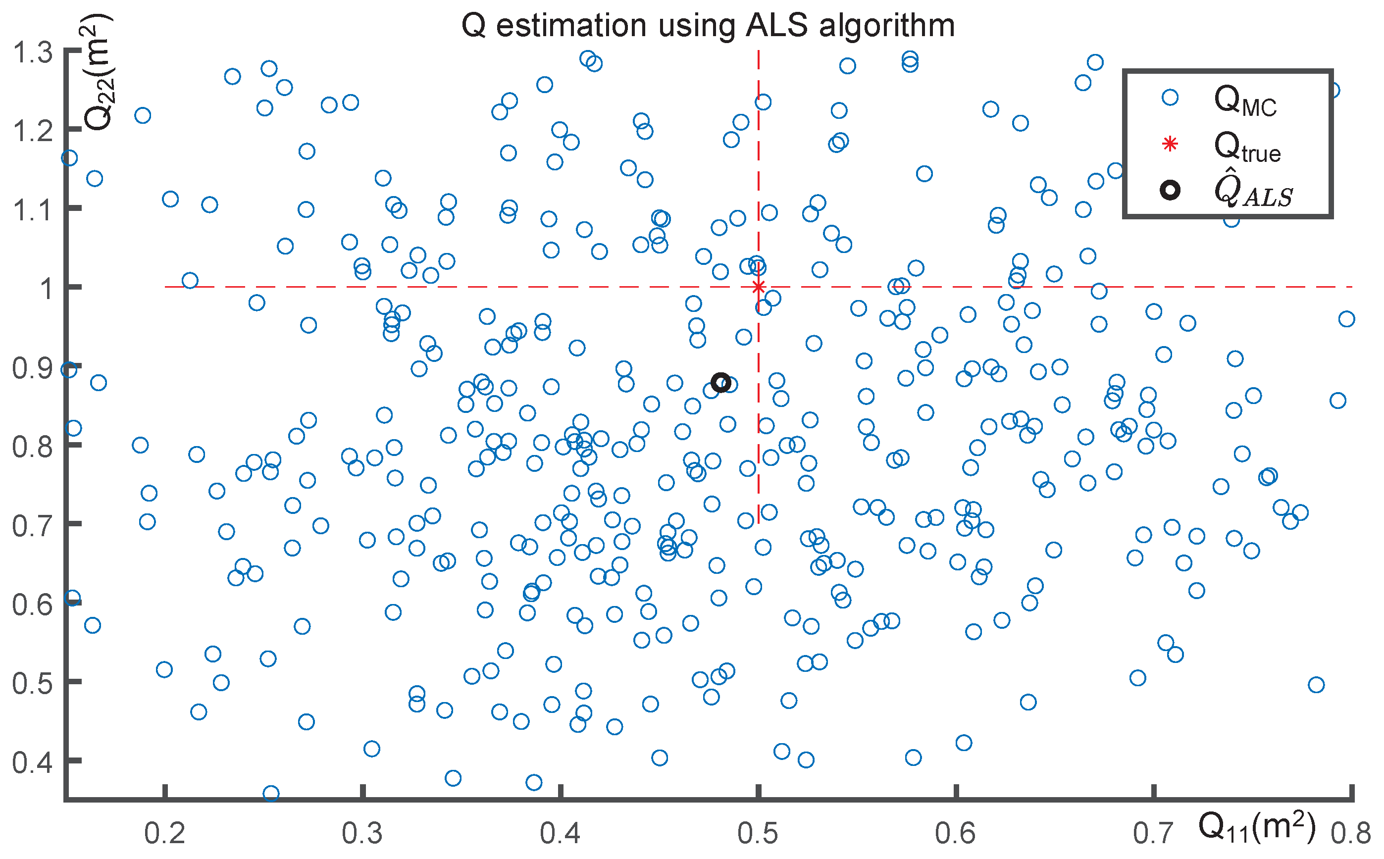
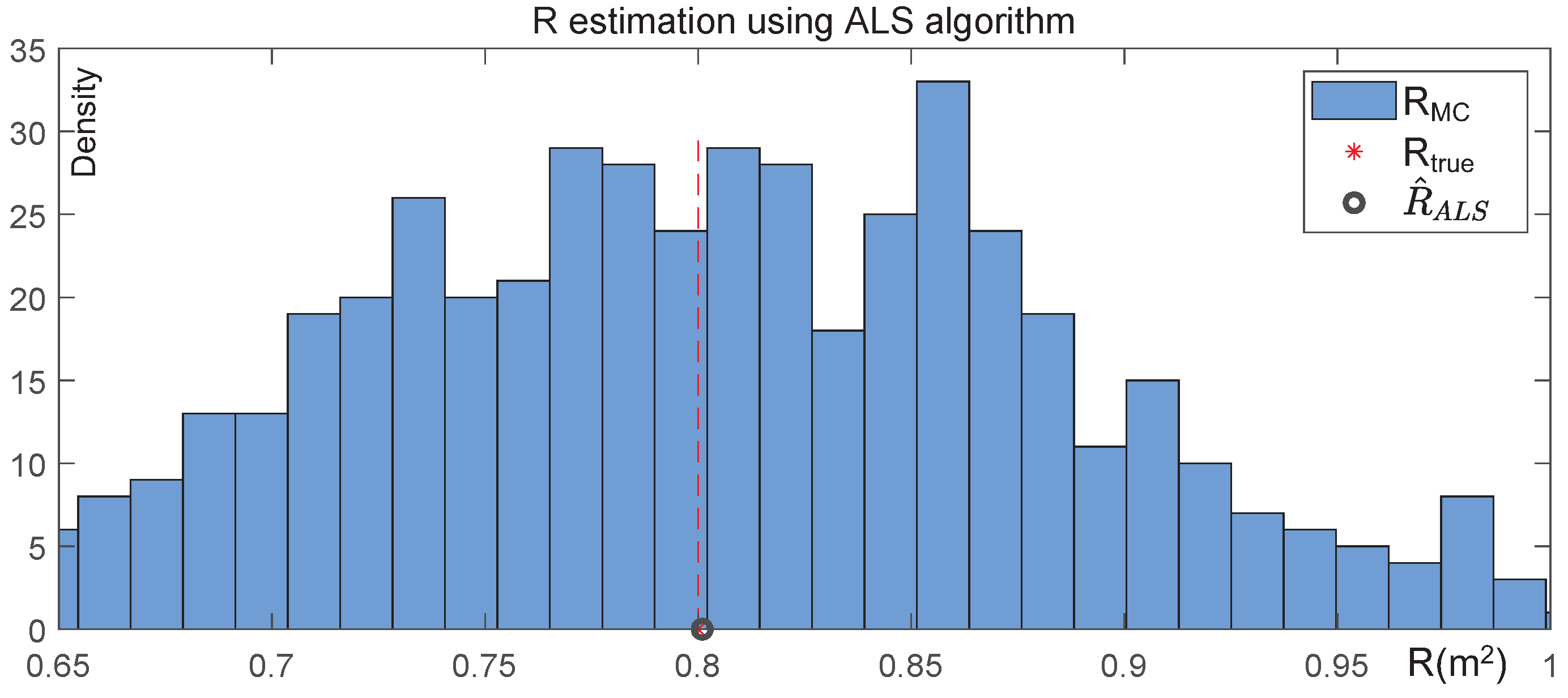
By setting the window size  N w  as 5, The empirical estimation of N-innovations autocovariance is computed as  b ^ = [ 2.019 , 1.144 , 1.177 , 0.861 , 0.794 ] T . Then according to the Equation (12), the estimated noise covariance matrix with 500 MC initialization is computed and stored as  Q ^ A L S , M C  and  R ^ A L S , M C , and the mean value of  Q ^ A L S , M C  and  R ^ A L S , M C  is  Q ^ A L S = 0.48 0.214 0.214 0.879  and  R ^ A L S = 0.801 .
The effectiveness of the estimated noise covariance matrices, based on 500 Monte Carlo simulations, is depicted in Figure 2 and Figure 3. Figure 2 plots the diagonal elements of the estimated model noise covariance matrix,  Q ^ 11  and  Q ^ 22 , on the x-axis and y-axis, respectively. Figure 3 presents the estimated measurement noise covariance matrix R on the x-axis, with the density of the Monte Carlo simulations displayed on the y-axis.
As indicated above, the noise covariance estimates with 500 MC initialization follow the Gaussian distribution where the mean value  Q A L S  and  R A L S  are near the true value. The results demonstrate that the ALS method can accurately estimate the noise covariance for the KF, and the ALS-KF framework which combines the Kalman filter with the ALS method is well-suited for real-world visual tracking applications where the underlying noise distributions are unknown.

4.2. Centroid-Based Moving Ball Tracking Subjected to Three Motions

The experiment on the video of a moving ball separately subjected to projectile motion, free-fall bouncing motion, and back-and-forth linear motion across the video is conducted to assess the performance of the proposed AKF-ALS algorithm. The video consists of 100 frames, with a resolution of 480 × 640 pixels.
  • Projectile motion following a parabolic path refers to the motion of an object thrown into the air and subject to downward acceleration due to gravity. The challenge in tracking such motion is the constantly changing speed and direction of the object.
  • Free-fall bouncing motion is the motion of an object falling under gravity and then bouncing back upwards. The challenge is the object’s velocity changes rapidly at the point of impact, which can be difficult for a tracking algorithm to handle.
  • Back-and-forth linear motion refers to an object moving to and fro along a straight line. The challenge is the abrupt change in velocity when the object changes direction.
For visual object tracking (VOT), these different types of motion pose unique challenges. Rapid changes in direction and velocity may affect the ability of a VOT system to accurately track an object. Therefore, the proposed AKF-ALS algorithm is applied to show the performance. In the algorithm, the background subtraction method is first applied to each frame in the video to detect the ball. The background is initialized as the first frame of the video, and an adaptive threshold is applied to the difference image to create a binary image. The connected components in the binary image are identified as potential objects, and the centroid of the largest component is stored as the location of the ball. Then the Kalman filter is used to track the ball’s movement, i.e., the centroid of a series of video frames. The ALS method is used to estimate the process and measurement noise covariance. The performance of the proposed method was compared with a standard Kalman filter with fixed noise covariance.
Specifically, we consider the state of the ball as its position and velocity, and the observation as the detected position of the ball from the background subtraction. Based on the kinematic equation, the relation between the position x and velocity  x ˙  can be written as follows:
x k = x k x ˙ k = x k 1 + x ˙ k 1 Δ t + 1 / 2 x ¨ k 1 Δ t 2 x ˙ k 1 + x ¨ k 1 Δ t
where  Δ t  is the sampling time and can be set as  0.2 . The 2-D kinetic equation can be shown for state  x k  as:
x k = x k y k x ˙ k y ˙ k = x k 1 + x ˙ k 1 Δ t + 1 / 2 x ¨ k 1 Δ t 2 y k 1 + y ˙ k 1 Δ t + 1 / 2 y ¨ k 1 Δ t 2 x ˙ k 1 + x ¨ k 1 Δ t y ˙ k 1 + y ¨ k 1 Δ t
which can be simplified as:
x k = 1 0 Δ t 0 0 1 0 Δ t 0 0 1 0 0 0 0 1 x k 1 + 1 / 2 Δ t 2 0 0 1 / 2 Δ t 2 Δ t 0 0 Δ t a k 1
where the transitional matrices F Γ  and H are defined as
F = 1 0 Δ t 0 0 1 0 Δ t 0 0 1 0 0 0 0 1 Γ = 1 / 2 Δ t 2 0 0 1 / 2 Δ t 2 Δ t 0 0 Δ t H = 1 0 0 0 0 1 0 0 .
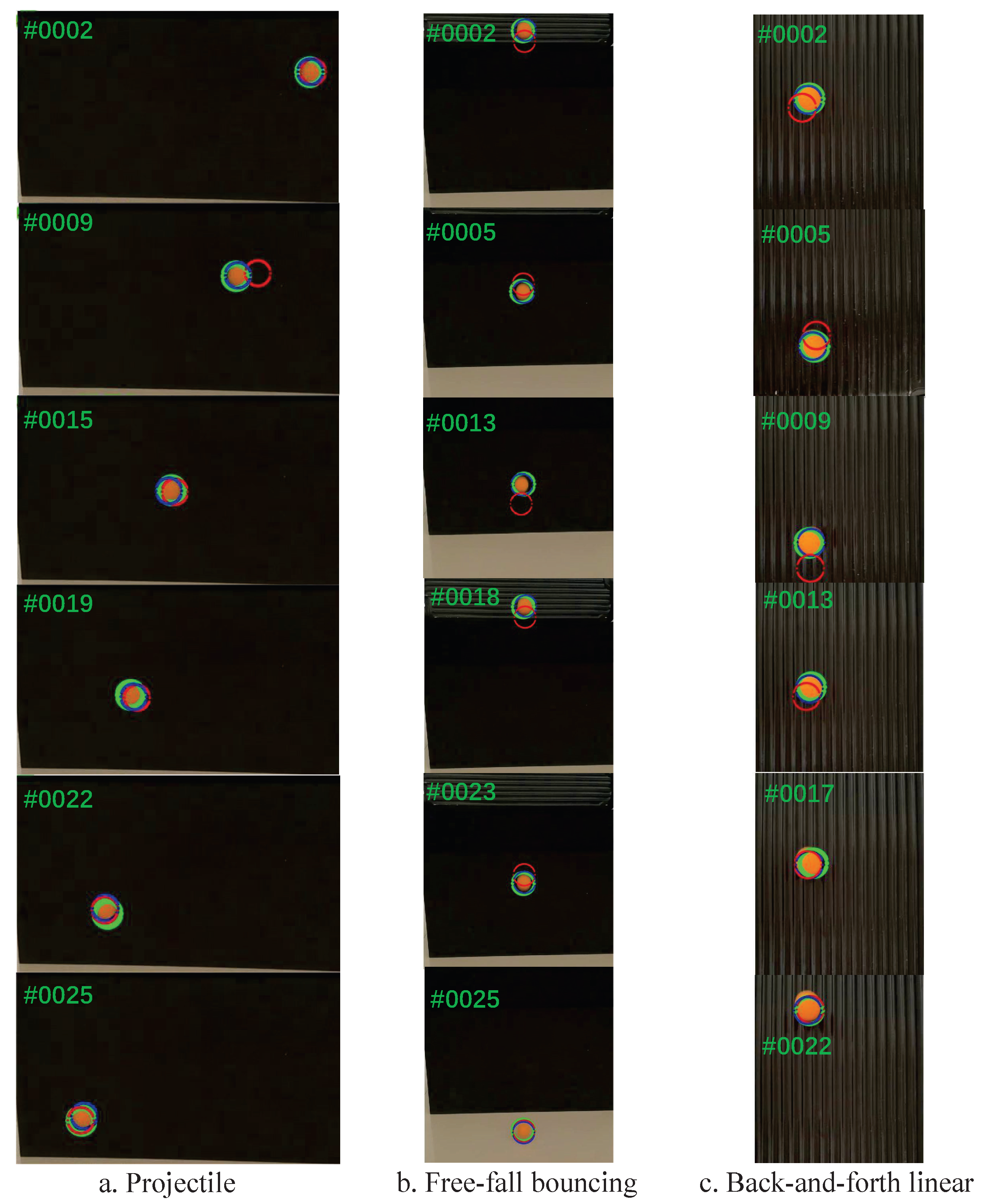
The performance of the proposed AKF-ALS-based VOT algorithm is compared to that of the traditional KF-based VOT algorithm, as introduced in [64], across three types of motion: projectile motion, free-fall with a bouncing trajectory, and linear back-and-forth motion. The KF-based VOT algorithm uses the same kinematic equation in (19), but the noise covariance is initially determined as a constant value, i.e.,  Q = 1  and  R = 0.5 . The comparative results are illustrated in Figure 4.
As indicated from the above figure, the proposed AKF-ALS algorithm shows improved robustness in handling constantly changing speed and direction, rapidly changing velocity, and the abrupt change in velocity when the object changes direction, while continuing tracking accurately after the change ends. As the tracking progresses, the performance of KF-based VOT approaches that of AKF-ALS-based VOT because the state covariance matrix approximates the steady-state value. This highlights the advantage of the proposed AKF-ALS-based VOT method in handling challenging conditions in visual object tracking.
The performance of the proposed ALS-KF-based VOT algorithm is evaluated using the root mean square error (RMSE) (in pixels) between the estimated position  x ^ 1 : 2 , t  (the first two elements) and the true position  x 1 : 2 , t  of the moving ball subjected to projectile motion, free-fall bouncing motion, and back-and-forth linear motion across the video, as shown in Table 1.
R M S E = 1 N t = 1 N ( x 1 : 2 , t x ^ 1 : 2 , t ) 2
The quantitative analysis of the table above reveals that AKF-ALS consistently achieves lower root mean square error (RMSE) values across various motion patterns. The RMSE for AKF-ALS is 1.05 pixels for projectile motion, significantly better than the 4.67 pixels of the standard KF. For free-fall bouncing motion, AKF-ALS records an RMSE of 2.76 pixels, in contrast to 8.35 pixels for the KF. Additionally, in back-and-forth linear motion scenarios, AKF-ALS demonstrates an RMSE of 0.89 pixels, outperforming the KF’s 2.31 pixels. The results show that the proposed AKF-ALS algorithm achieves a lower RMSE compared to a standard KF VOT algorithm with fixed noise covariance, demonstrating the proposed method outperformed the standard Kalman filter in terms of RMSE.

4.3. Bounding Box-Based Pedestrian Tracking with Occlusions

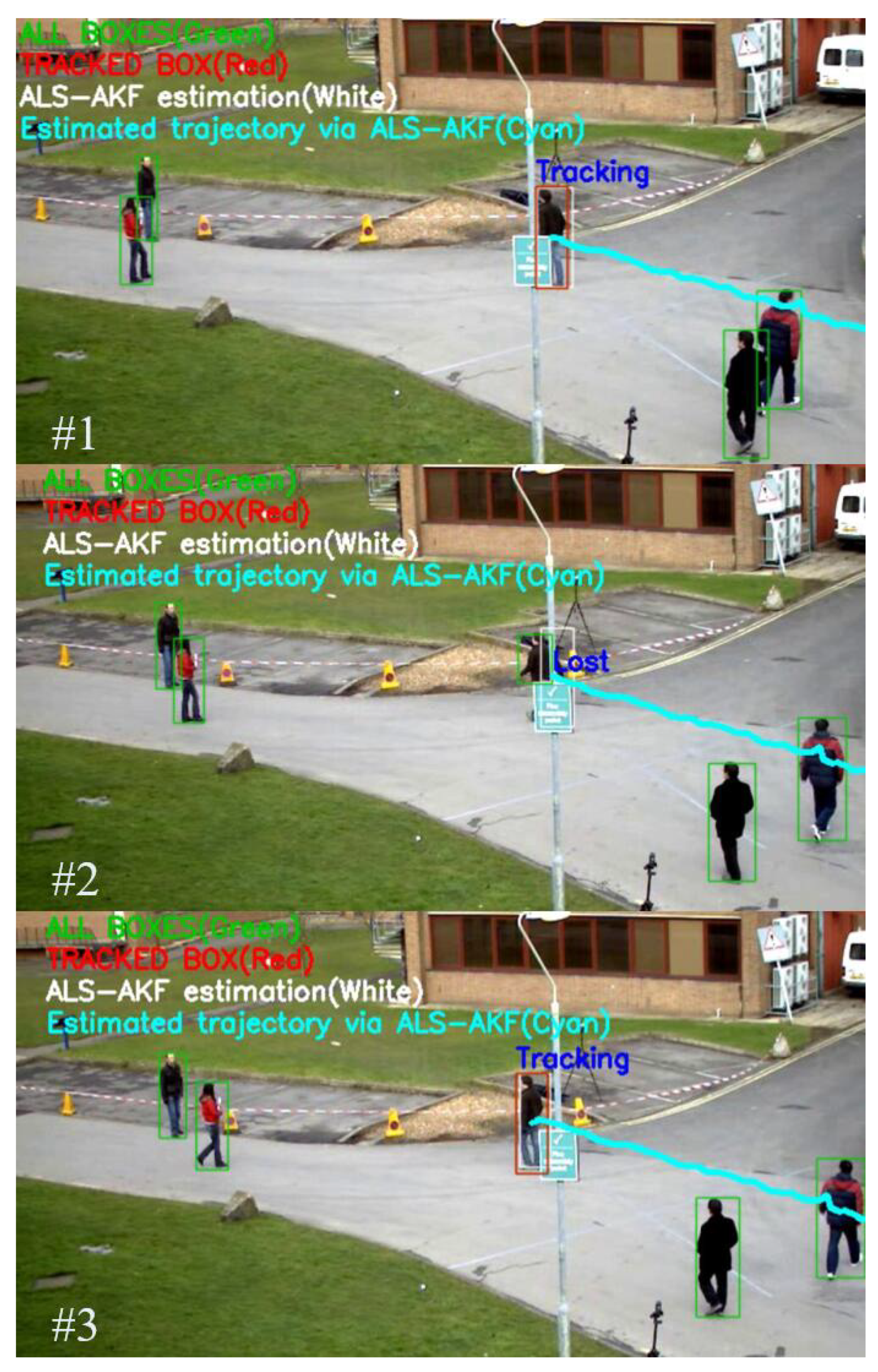
The simulation was also conducted on the PETS09-S2L1 dataset [65] within the MOT-15 challenge, a complex scenario with up to eight pedestrians engaging in unusual patterns. The IOU matching utilized the detection box from the previous frame to compute the IOU with the current frame detections. A threshold of  I O U Threshold = 0.3  was set for a match to be considered valid. If the IOU matching failed to find a maximum value due to occlusion, the Kalman filter’s prediction was used to estimate the target’s new position and continue tracking. However, the KF-based VOT algorithm failed to maintain tracking under occlusion conditions.
The AKF-ALS VOT algorithm demonstrated robustness in maintaining the identity of the pedestrian target even when the IOU matching failed due to occlusion due to its dynamic covariance estimation, which allows the filter to adapt its parameters in response to the evolving state of the system. This adaptive mechanism is crucial for handling occlusions and erratic pedestrian movements. The AKF-ALS VOT algorithm improves upon the standard KF VOT by dynamically adjusting the process and measurement noise covariances. The state vector remains consistent with the classic AKF, with the following representation:
X = [ x , y , h , w , x ˙ , y ˙ ] T
where x and y denote the horizontal and vertical position of the pedestrian in the video frame (in pixels), respectively, and  x ˙  and  y ˙  denote the horizontal and vertical velocity of the pedestrian (in pixels per frame). h and w denote the height and width of the bounding box around the pedestrian (in pixels), respectively.
The ALS algorithm updates the process noise covariance matrix Q and the observation noise covariance matrix R iteratively. The innovation sequence is used to calculate the autocovariance, which in turn adjusts Q and R to respond to abrupt changes in the tracked object’s motion. The trajectory is shown in Figure 5.
As indicated by the figure, the tracking of pedestrians in scenarios obstructed by objects such as a light pole, can present challenges for bounding box detection methods. However, the implementation of the adaptive Kalman filter with adaptive least squares (AKF-ALS) algorithm demonstrates robustness in tracking despite failures in bounding box detection under such conditions.
To demonstrate the comparative performance of the accuracy and robustness, we use the RMSE in (23), the identity switches, and the track fragmentation as the metrics. The identity switches metric measures the number of times the tracking algorithm incorrectly switches the identity of the tracked object. Fewer identity switches indicate a more robust tracking performance. The track fragmentation evaluates the continuity of the tracking throughout the sequence. Lower numbers imply fewer instances where tracks are broken and later reacquired. We compare the proposed ALS-AKF algorithm with the classic adaptive KF algorithm using Otsu’s method in [66], as shown in Table 2.
As is indicated from the table above, the AKF-ALS VOT algorithm demonstrated a markedly higher precision with a root mean square error (RMSE) of only 5.5 pixels, compared to the classic AKF VOT’s 10.7 pixels. Robustness in maintaining pedestrian identity was also significantly improved in the AKF-ALS VOT, which had a mere single identity switch, whereas the classic AKF VOT recorded eight. Additionally, the AKF-ALS VOT showed greater continuity in tracking with only two instances of track fragmentation, in contrast to the classic AKF VOT’s eight, indicating a more stable tracking performance throughout the sequences. These enhancements are likely due to the AKF-ALS’s iterative updates to the process and observation noise covariance matrices, enabling it to adeptly adjust to sudden changes in the tracked object’s motion.

5. Conclusions

In conclusion, the AKF-ALS algorithm introduced in this paper represents a significant advancement in the field of real-time visual object tracking. By integrating the autocovariance least squares estimation method with an adaptive Kalman filter, we have demonstrated a robust approach to tracking that compensates for system model mismatches and invalid offline calibration, which are critical in dynamic environments. The computational complexity analysis indicates that AKF-ALS is efficient enough for real-time applications, striking an optimal balance between computational load and tracking accuracy. Our experimental results have shown that the AKF-ALS algorithm exhibits superior performance over traditional Kalman filter methods that rely on fixed noise statistics. The algorithm’s capability to adapt to changing noise covariances in real-time ensures greater accuracy in tracking the centroid of a moving object under various motion patterns, including projectile motion, free-falling with bounces, and linear back-and-forth motion. Experimental results on the complex PETS09-S2L1 dataset from the MOT-15 challenge demonstrate that the AKF-ALS VOT algorithm is capable of tracking pedestrians with occlusion where traditional methods fail. The algorithm’s dynamic adaptation to changing noise covariances in real-time significantly enhances accuracy and reliability in tracking various motion patterns. Overall, the AKF-ALS algorithm’s ability to iteratively refine noise covariances and adjust to abrupt motion changes makes it an excellent candidate for autonomous vehicles or mobile robotics.
Future work should focus on expanding the validation of the AKF-ALS algorithm across a broader range of applications, including those with more complex and non-linear object dynamics. Additionally, further research could explore the integration of this algorithm with deep learning techniques to enhance tracking performance in highly cluttered and dynamic visual scenes.

Author Contributions

Conceptualization, J.L. and X.X.; methodology, J.L. and B.J.; software, J.L. and Z.J.; validation, J.L. and B.J.; writing—original draft preparation, J.L. and X.X. All authors have read and agreed to the published version of the manuscript.

Funding

This research is supported in part by the National Natural Science Foundation of China under grant 61803034, 61973035, R&D Program of Beijing Municipal Education Commission (KM202311417006), and the National Natural Science Foundation of China Basic Science Center Program under Grant 62088101.

Institutional Review Board Statement

Not applicable.

Informed Consent Statement

Not applicable.

Data Availability Statement

The dataset established is available upon requests from the corresponding author. The data are not publicly available due to the data are generated randomly based on constraints and parameter settings.

Conflicts of Interest

The authors declare no conflicts of interest.

References

  1. Yadav, S.P. Vision-based detection, tracking, and classification of vehicles. IEIE Trans. Smart Process. Comput. 2020, 9, 427–434. [Google Scholar] [CrossRef]
  2. Abdulrahim, K.; Salam, R.A. Traffic surveillance: A review of vision based vehicle detection, recognition and tracking. Int. J. Appl. Eng. Res. 2016, 11, 713–726. [Google Scholar]
  3. Gad, A.; Basmaji, T.; Yaghi, M.; Alheeh, H.; Alkhedher, M.; Ghazal, M. Multiple Object Tracking in Robotic Applications: Trends and Challenges. Appl. Sci. 2022, 12, 9408. [Google Scholar] [CrossRef]
  4. Gammulle, H.; Ahmedt-Aristizabal, D.; Denman, S.; Tychsen-Smith, L.; Petersson, L.; Fookes, C. Continuous human action recognition for human-machine interaction: A review. ACM Comput. Surv. 2023, 55, 1–38. [Google Scholar] [CrossRef]
  5. Dong, X.; Shen, J.; Yu, D.; Wang, W.; Liu, J.; Huang, H. Occlusion-aware real-time object tracking. IEEE Trans. Multimed. 2016, 19, 763–771. [Google Scholar] [CrossRef]
  6. Setitra, I.; Larabi, S. Background subtraction algorithms with post-processing: A review. In Proceedings of the 2014 22nd International Conference on Pattern Recognition, Stockholm, Sweden, 24–28 August 2014; pp. 2436–2441. [Google Scholar]
  7. Shaikh, S.H.; Saeed, K.; Chaki, N.; Shaikh, S.H.; Saeed, K.; Chaki, N. Moving Object Detection Using Background Subtraction. In Moving Object Detection Using Background Subtraction; SpringerBriefs in Computer Science; Springer: Cham, Switzerland, 2014. [Google Scholar] [CrossRef]
  8. Bouwmans, T.; Javed, S.; Sultana, M.; Jung, S.K. Deep neural network concepts for background subtraction: A systematic review and comparative evaluation. Neural Netw. 2019, 117, 8–66. [Google Scholar] [CrossRef]
  9. Kalsotra, R.; Arora, S. Background subtraction for moving object detection: Explorations of recent developments and challenges. Vis. Comput. 2022, 38, 4151–4178. [Google Scholar] [CrossRef]
  10. Zhang, H.; Wu, K. A vehicle detection algorithm based on three-frame differencing and background subtraction. In Proceedings of the 2012 Fifth International Symposium on Computational Intelligence and Design, Hangzhou, China, 28–29 October 2012; Volume 1, pp. 148–151. [Google Scholar] [CrossRef]
  11. Li, J.; Pan, Z.M.; Zhang, Z.H.; Zhang, H. Dynamic ARMA-based background subtraction for moving objects detection. IEEE Access 2019, 7, 128659–128668. [Google Scholar] [CrossRef]
  12. Zhang, R.; Gong, W.; Grzeda, V.; Yaworski, A.; Greenspan, M. An adaptive learning rate method for improving adaptability of background models. IEEE Signal Process. Lett. 2013, 20, 1266–1269. [Google Scholar] [CrossRef]
  13. Shi, P.; Jones, E.G.; Zhu, Q. Median model for background subtraction in intelligent transportation system. In Image Processing: Algorithms and Systems III; SPIE: Bellingham, WA, USA, 2004; Volume 5298, pp. 168–176. [Google Scholar]
  14. Li, X.; Ng, M.K.; Yuan, X. Median filtering-based methods for static background extraction from surveillance video. Numer. Linear Algebra Appl. 2015, 22, 845–865. [Google Scholar] [CrossRef]
  15. Roy, S.M.; Ghosh, A. Real-time adaptive histogram min-max bucket (HMMB) model for background subtraction. IEEE Trans. Circuits Syst. Video Technol. 2017, 28, 1513–1525. [Google Scholar] [CrossRef]
  16. Stauffer, C.; Grimson, W.E.L. Adaptive background mixture models for real-time tracking. In Proceedings of the 1999 IEEE Computer Society Conference on Computer Vision and Pattern Recognition (Cat. No PR00149), Fort Collins, CO, USA, 23–25 June 1999; Volume 2, pp. 246–252. [Google Scholar]
  17. Zivkovic, Z.; Van Der Heijden, F. Efficient adaptive density estimation per image pixel for the task of background subtraction. Pattern Recognit. Lett. 2006, 27, 773–780. [Google Scholar] [CrossRef]
  18. Sheikh, Y.; Shah, M. Bayesian modeling of dynamic scenes for object detection. IEEE Trans. Pattern Anal. Mach. Intell. 2005, 27, 1778–1792. [Google Scholar] [CrossRef]
  19. Han, B.; Comaniciu, D.; Zhu, Y.; Davis, L.S. Sequential kernel density approximation and its application to real-time visual tracking. IEEE Trans. Pattern Anal. Mach. Intell. 2008, 30, 1186–1197. [Google Scholar] [PubMed]
  20. Zhu, Q.; Shao, L.; Li, Q.; Xie, Y. Recursive kernel density estimation for modeling the background and segmenting moving objects. In Proceedings of the 2013 IEEE International Conference on Acoustics, Speech and Signal Processing, Vancouver, BC, Canada, 26–31 May 2013; pp. 1769–1772. [Google Scholar]
  21. Lin, H.H.; Liu, T.L.; Chuang, J.H. A probabilistic SVM approach for background scene initialization. In Proceedings of the International Conference on Image Processing, Rochester, NY, USA, 22–25 September 2002; Volume 3, pp. 893–896. [Google Scholar]
  22. Cheng, L.; Gong, M.; Schuurmans, D.; Caelli, T. Real-time discriminative background subtraction. IEEE Trans. Image Process. 2010, 20, 1401–1414. [Google Scholar] [CrossRef]
  23. Bouwmans, T. Subspace learning for background modeling: A survey. Recent Patents Comput. Sci. 2009, 2, 223–234. [Google Scholar] [CrossRef]
  24. Djerida, A.; Zhao, Z.; Zhao, J. Background subtraction in dynamic scenes using the dynamic principal component analysis. IET Image Process. 2020, 14, 245–255. [Google Scholar] [CrossRef]
  25. Buccolieri, F.; Distante, C.; Leone, A. Human posture recognition using active contours and radial basis function neural network. In Proceedings of the IEEE Conference on Advanced Video and Signal Based Surveillance, Como, Italy, 15–16 September 2005; pp. 213–218. [Google Scholar]
  26. Maddalena, L.; Petrosino, A. A self-organizing approach to background subtraction for visual surveillance applications. IEEE Trans. Image Process. 2008, 17, 1168–1177. [Google Scholar] [CrossRef] [PubMed]
  27. Gemignani, G.; Rozza, A. A robust approach for the background subtraction based on multi-layered self-organizing maps. IEEE Trans. Image Process. 2016, 25, 5239–5251. [Google Scholar] [CrossRef]
  28. Braham, M.; Van Droogenbroeck, M. Deep background subtraction with scene-specific convolutional neural networks. In Proceedings of the 2016 International Conference on Systems, Signals and Image Processing (IWSSIP), Bratislava, Slovakia, 23–25 May 2016; pp. 1–4. [Google Scholar]
  29. Babaee, M.; Dinh, D.T.; Rigoll, G. A deep convolutional neural network for video sequence background subtraction. Pattern Recognit. 2018, 76, 635–649. [Google Scholar] [CrossRef]
  30. Bakkay, M.C.; Rashwan, H.A.; Salmane, H.; Khoudour, L.; Puig, D.; Ruichek, Y. BSCGAN: Deep background subtraction with conditional generative adversarial networks. In Proceedings of the 2018 25th IEEE International Conference on Image Processing (ICIP), Athens, Greece, 7–10 October 2018; pp. 4018–4022. [Google Scholar]
  31. Sultana, M.; Mahmood, A.; Bouwmans, T.; Jung, S.K. Dynamic background subtraction using least square adversarial learning. In Proceedings of the 2020 IEEE International Conference on Image Processing (ICIP), Abu Dhabi, United Arab Emirates, 25–28 October 2020; pp. 3204–3208. [Google Scholar]
  32. McHugh, J.M.; Konrad, J.; Saligrama, V.; Jodoin, P.M. Foreground-adaptive background subtraction. IEEE Signal Process. Lett. 2009, 16, 390–393. [Google Scholar] [CrossRef]
  33. Li, X.; Hu, W.; Shen, C.; Zhang, Z.; Dick, A.; Hengel, A.V.D. A survey of appearance models in visual object tracking. ACM Trans. Intell. Syst. Technol. (TIST) 2013, 4, 1–48. [Google Scholar] [CrossRef]
  34. Fiaz, M.; Mahmood, A.; Javed, S.; Jung, S.K. Handcrafted and deep trackers: Recent visual object tracking approaches and trends. ACM Comput. Surv. (CSUR) 2019, 52, 1–44. [Google Scholar] [CrossRef]
  35. Javed, S.; Danelljan, M.; Khan, F.S.; Khan, M.H.; Felsberg, M.; Matas, J. Visual object tracking with discriminative filters and siamese networks: A survey and outlook. IEEE Trans. Pattern Anal. Mach. Intell. 2022, 45, 6552–6574. [Google Scholar] [CrossRef]
  36. Ondrašovič, M.; Tarábek, P. Siamese visual object tracking: A survey. IEEE Access 2021, 9, 110149–110172. [Google Scholar] [CrossRef]
  37. Chen, F.; Wang, X.; Zhao, Y.; Lv, S.; Niu, X. Visual object tracking: A survey. Comput. Vis. Image Underst. 2022, 222, 103508. [Google Scholar] [CrossRef]
  38. Zhou, H.; Yuan, Y.; Shi, C. Object tracking using SIFT features and mean shift. Comput. Vis. Image Underst. 2009, 113, 345–352. [Google Scholar] [CrossRef]
  39. Khan, Z.H.; Gu, I.Y.H.; Backhouse, A.G. Robust visual object tracking using multi-mode anisotropic mean shift and particle filters. IEEE Trans. Circuits Syst. Video Technol. 2011, 21, 74–87. [Google Scholar] [CrossRef]
  40. Cai, Z.; Gu, Z.; Yu, Z.L.; Liu, H.; Zhang, K. A real-time visual object tracking system based on Kalman filter and MB-LBP feature matching. Multimed. Tools Appl. 2016, 75, 2393–2409. [Google Scholar] [CrossRef]
  41. Farahi, F.; Yazdi, H.S. Probabilistic Kalman filter for moving object tracking. Signal Process. Image Commun. 2020, 82, 115751. [Google Scholar] [CrossRef]
  42. Kim, T.; Park, T.H. Extended Kalman filter (EKF) design for vehicle position tracking using reliability function of radar and lidar. Sensors 2020, 20, 4126. [Google Scholar] [CrossRef] [PubMed]
  43. Zhou, Z.; Wu, D.; Zhu, Z. Object tracking based on Kalman particle filter with LSSVR. Optik 2016, 127, 613–619. [Google Scholar] [CrossRef]
  44. Iswanto, I.A.; Li, B. Visual object tracking based on mean-shift and particle-Kalman filter. Procedia Comput. Sci. 2017, 116, 587–595. [Google Scholar] [CrossRef]
  45. Rao, G.M.; Satyanarayana, C. Visual object target tracking using particle filter: A survey. Int. J. Image Graph. Signal Process. 2013, 5, 1250. [Google Scholar] [CrossRef]
  46. Kalman, R.E. A New Approach to Linear Filtering and Prediction Problems. J. Basic Eng. 1960, 82, 35–45. [Google Scholar] [CrossRef]
  47. Chen, J.; Li, J.; Yang, S.; Deng, F. Weighted optimization-based distributed Kalman filter for nonlinear target tracking in collaborative sensor networks. IEEE Trans. Cybern. 2016, 47, 3892–3905. [Google Scholar] [CrossRef]
  48. Zheng, B.; Fu, P.; Li, B.; Yuan, X. A robust adaptive unscented Kalman filter for nonlinear estimation with uncertain noise covariance. Sensors 2018, 18, 808. [Google Scholar] [CrossRef] [PubMed]
  49. Jeong, J.; Yoon, T.S.; Park, J.B. Mean shift tracker combined with online learning-based detector and Kalman filtering for real-time tracking. Expert Syst. Appl. 2017, 79, 194–206. [Google Scholar] [CrossRef]
  50. Sun, J.; Xu, X.; Liu, Y.; Zhang, T.; Li, Y. FOG random drift signal denoising based on the improved AR model and modified Sage-Husa adaptive Kalman filter. Sensors 2016, 16, 1073. [Google Scholar] [CrossRef]
  51. Särkkä, S.; Nummenmaa, A. Recursive Noise Adaptive Kalman Filtering by Variational Bayesian Approximations. IEEE Trans. Autom. Control 2009, 54, 596–600. [Google Scholar] [CrossRef]
  52. Kashyap, R. Maximum likelihood identification of stochastic linear systems. IEEE Trans. Autom. Control 1970, 15, 25–34. [Google Scholar] [CrossRef]
  53. Zagrobelny, M.A.; Rawlings, J.B. Identifying the uncertainty structure using maximum likelihood estimation. In Proceedings of the 2015 American Control Conference (ACC), Chicago, IL, USA, 1–3 July 2015; pp. 422–427. [Google Scholar]
  54. Myers, K.; Tapley, B. Adaptive sequential estimation with unknown noise statistics. IEEE Trans. Autom. Control 1976, 21, 520–523. [Google Scholar] [CrossRef]
  55. Solonen, A.; Hakkarainen, J.; Ilin, A.; Abbas, M.; Bibov, A. Estimating model error covariance matrix parameters in extended Kalman filtering. Nonlinear Process. Geophys. 2014, 21, 919–927. [Google Scholar] [CrossRef]
  56. Yu, C.; Verhaegen, M. Subspace identification of distributed clusters of homogeneous systems. IEEE Trans. Autom. Control 2016, 62, 463–468. [Google Scholar] [CrossRef]
  57. Mehra, R.K. On the identification of variances and adaptive Kalman filtering. IEEE Trans. Autom. Control 1970, 15, 175–184. [Google Scholar] [CrossRef]
  58. Odelson, B.J.; Rajamani, M.R.; Rawlings, J.B. A new autocovariance least-squares method for estimating noise covariances. Automatica 2006, 42, 303–308. [Google Scholar] [CrossRef]
  59. Duník, J.; Straka, O.; Simandl, M. On Autocovariance Least-Squares Method for Noise Covariance Matrices Estimation. IEEE Trans. Autom. Control 2017, 62, 967–972. [Google Scholar] [CrossRef]
  60. Duník, J.; Straka, O.; Kost, O.; Havlík, J. Noise covariance matrices in state-space models: A survey and comparison of estimation methods—Part I. Int. J. Adapt. Control Signal Process. 2017, 31, 1505–1543. [Google Scholar] [CrossRef]
  61. Li, J.; Ma, N.; Deng, F. Distributed noise covariance matrices estimation in sensor networks. In Proceedings of the 2020 59th IEEE Conference on Decision and Control (CDC), Jeju, Republic of Korea, 14–18 December 2020; pp. 1158–1163. [Google Scholar]
  62. Arnold, T.J.; Rawlings, J.B. Tractable Calculation and Estimation of the Optimal Weighting Matrix for ALS Problems. IEEE Trans. Autom. Control 2021, 67, 6045–6052. [Google Scholar] [CrossRef]
  63. Meng, Y.; Gao, S.; Zhong, Y.; Hu, G.; Subic, A. Covariance matching based adaptive unscented Kalman filter for direct filtering in INS/GNSS integration. Acta Astronaut. 2016, 120, 171–181. [Google Scholar] [CrossRef]
  64. Fu, Z.; Han, Y. Centroid weighted Kalman filter for visual object tracking. Measurement 2012, 45, 650–655. [Google Scholar] [CrossRef]
  65. Ferryman, J.; Shahrokni, A. PETS2009: Dataset and challenge. In Proceedings of the 2009 Twelfth IEEE International Workshop on Performance Evaluation of Tracking and Surveillance, Snowbird, UT, USA, 7–9 December 2009; pp. 1–6. [Google Scholar] [CrossRef]
  66. Tripathi, R.P.; Singh, A.K. Moving Object Tracking Using Optimal Adaptive Kalman Filter Based on Otsu’s Method. In Innovations in Electronics and Communication Engineering, Proceedings of the 8th ICIECE 2019, Hyderabad, India, 2–3 August 2019; Springer: Singapore, 2020; pp. 429–435. [Google Scholar]
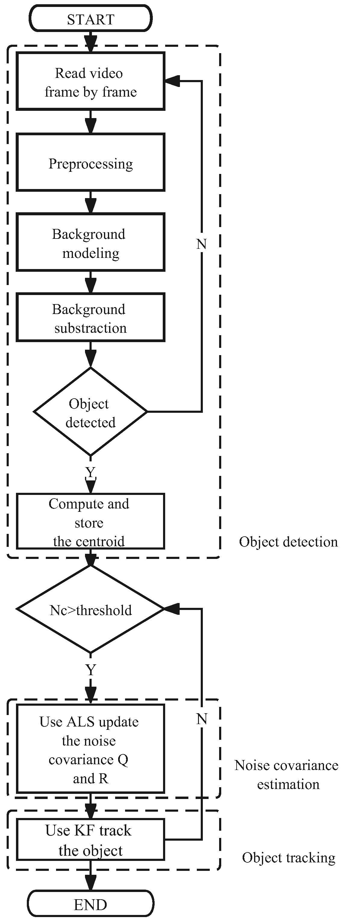
Figure 1. Flowchart of the ALS-KF based VOT algorithm.
Applsci 14 01045 g001
Figure 2. Performance of model noise covariance estimation  Q A L S  using ALS algorithm over 500 Monte Carlo simulations. The blue dots denote the estimated diagonal-form model noise covariance matrix  Q M C = d i a g ( Q ^ 11 , Q ^ 22 )  over each Monte Carlo simulation, where the x-axis and y-axis represent the first and second diagonal elements respectively. The black bold dot is the model noise covariance estimate  Q ^ A L S  via the ALS algorithm. The intersection of two red dotted lines denotes the true noise covariance  Q t r u e .
Applsci 14 01045 g002
Figure 3. Performance of measurement noise covariance estimation  R A L S  using ALS algorithm over 500 Monte Carlo simulations. The blue bars denote the estimated measurement noise covariance value  R M C  over each Monte Carlo simulation, where the x-axis and y-axis respectively represent the measurement noise covariance value and the probabilistic density. The black bold dot is the measurement noise covariance estimate  Q ^ A L S  via the ALS algorithm. The intersection of the red dotted line and x-axis denotes the true noise covariance  Q t r u e .
Applsci 14 01045 g003
Figure 4. VOT using the proposed AKF-ALS algorithm and traditional KF algorithm. The green, blue, and red circles, respectively, represent the circle of the ball with true centroid, with estimated centroid using AKF-ALS algorithm, and with estimated centroid using KF algorithm.
Applsci 14 01045 g004
Figure 5. Bounding box-based pedestrian tracking with occlusions using AKF-ALS algorithm.
Applsci 14 01045 g005
Table 1. Comparisons of RMSE (in pixels) between AKF-ALS-based and KF-based VOT subjected to projectile motion, free-fall bouncing motion, and back-and-forth linear motion.
RMSE (in Pixels)ProjectileFree-Fall BouncingBack-and-Forth Linear
AKF-ALS1.052.760.89
KF4.678.352.31
Table 2. Comparisons of RMSE (in pixels), between AKF-ALS-based and KF-based VOT algorithm in pedestrian tracking with occlusions.
MetricAKF ALS VOTClassic AKF VOT [66]
RMSE5.5 pixels10.7 pixels
Identity switches18
Track fragmentation28
Disclaimer/Publisher’s Note: The statements, opinions and data contained in all publications are solely those of the individual author(s) and contributor(s) and not of MDPI and/or the editor(s). MDPI and/or the editor(s) disclaim responsibility for any injury to people or property resulting from any ideas, methods, instructions or products referred to in the content.