Suitable Integral Sampling for Bandpass-Sampling Time-Modulated Fourier Transform Spectroscopy

Abstract

For traditional Fourier transform (FTS), its integral sampling usually meets the Spectral Modulation Transfer Function (SMTF) criterion. However, for bandpass-sampling Fourier transform spectroscopy (BPS-FTS), based on our analysis, the integral sampling condition derived from the Spectral Modulation Transfer Function (SMTF) is excessively stringent. In other words, the interval of the integral sampling time that fulfills the tolerance requirements for the reconstructed spectrum is very narrow. There are numerous integration sampling time intervals outside this range that still meet the tolerance requirements for the reconstructed spectrum. In this paper, through theoretical modeling, we propose a method based on average |SMTF| as the selection criterion for the integration sampling time. Through simulation analysis, it is evident that the intervals and range of the integral sampling time obtained via this method are more accurate, ensuring the tolerance requirements of the reconstructed spectrum. Under these intervals, when conducting integral sampling on the interferogram, the spectral deviation of the reconstructed spectrum is minimal, and the Spectral Correlation Mapper (SCM) is nearly equal to one. This indicates that compared with the SMTF criterion in traditional FTS, this method is more suitable for the characteristics of BPS-FTS. The analysis in this paper can provide theoretical and simulation support for the implementation of BPS-FTS.

1. Introduction

FTS has been widely applied in various fields, including scientific research, medicine manufacturing, gas sensing, and material analysis [1,2,3,4,5,6]. In order to improve interferogram modulation, post-dispersed Fourier transform spectroscopy has been proposed and comprehensively explored, finding successful applications in astronomical observations; however, at this time, interferogram sampling is still based on the Nyquist sampling theorem. Subsequently, following the development of bandpass sampling theory, this method has been applied for the analysis of post-dispersed FTS, known as BPS-FTS. According to bandpass sampling theory, the interferogram from post-dispersed FTS has the characteristics of a small number of sampling points and a large sampling interval along the optical path difference. Due to its attractive advantages, BPS-FTS has been widely studied and different types of BPS-FTS have been proposed [7,8,9,10,11,12,13,14,15]. Compared to post-dispersed FTS, BPS-FTS has many theoretical issues and technical challenges that still need to be analyzed and addressed, which arise from bandpass sampling and limit the implementation of BPS-FTS.

However, whether FTS is conducted using post-dispersed FTS or BPS-FTS, in order to ensure a high signal-to-noise ratio of the reconstructed spectrum, each sampling point of the interferogram needs to reach a sufficient optical energy. As a result, each sampling point is typically held for a certain integration time during interferogram sampling, leading to the hypothetical impulse sampling becoming rectangular sampling when the optical path difference (OPD) changes with time. Normally, a longer integration time in interferogram sampling results in a higher signal-to-noise ratio in the reconstructed spectrum. For traditional FTS, the integration time can be set arbitrarily as long as the interval between two sampling points satisfies the Nyquist sampling theorem, ensuring that the restored spectra fall within the acceptable error range of the spectrum. However, for BPS-FTS, since it adheres to the bandpass sampling theorem, its sampling interval is considerably larger than that mandated by the traditional Nyquist sampling theorem. While it offers the potential for a longer integration time, it remains unclear whether this integration time can be set arbitrarily, as in the case of Nyquist’s theorem. It is also unknown whether arbitrary settings will cause distortion of the spectrum. On the other hand, the longer integration sampling time may lead to the interferogram not satisfying the requirements of bandpass sampling theory. Therefore, it is worth determining what kind of integration sampling time is suitable for BPS-FTS. However, no studies in the existing literature have addressed this issue. Therefore, integral sampling in the context of BPS-FTS has been studied through theoretical modeling, analysis, and simulation in this paper. It is hoped that this work can provide theoretical and simulation support for the implementation of BPS-FTS.

In this study, a BPS-FTS method based on Michelson moving mirror FTS [14] is used for modeling and simulation. By employing bandpass sampling [16,17,18] instead of traditional Nyquist sampling [19,20,21,22,23,24] for each narrowband spectrum, we can reduce the number of sampling points across the entire optical path difference of the interferogram. We provide a theoretical derivation of changes in the interference model caused via integral sampling under bandpass sampling theory. Furthermore, using the SMTF criterion [25,26,27], we discuss and analyze suitable integral sampling conditions that meet the distortion tolerance for the reconstructed spectrum. Sampled interferograms with different integral sampling times and the corresponding reconstructed spectra are also modeled and analyzed. How the accuracy of the reconstructed spectrum varies with the integral sampling times of the interferogram is investigated, and a new criterion for determining a suitable integral interferogram sampling time for BPS-FTS is acquired. The simulation results demonstrate that the proposed criterion is more universally applicable for integral time sampling in BPS-FTS.

2. Principle of BPS-FTS

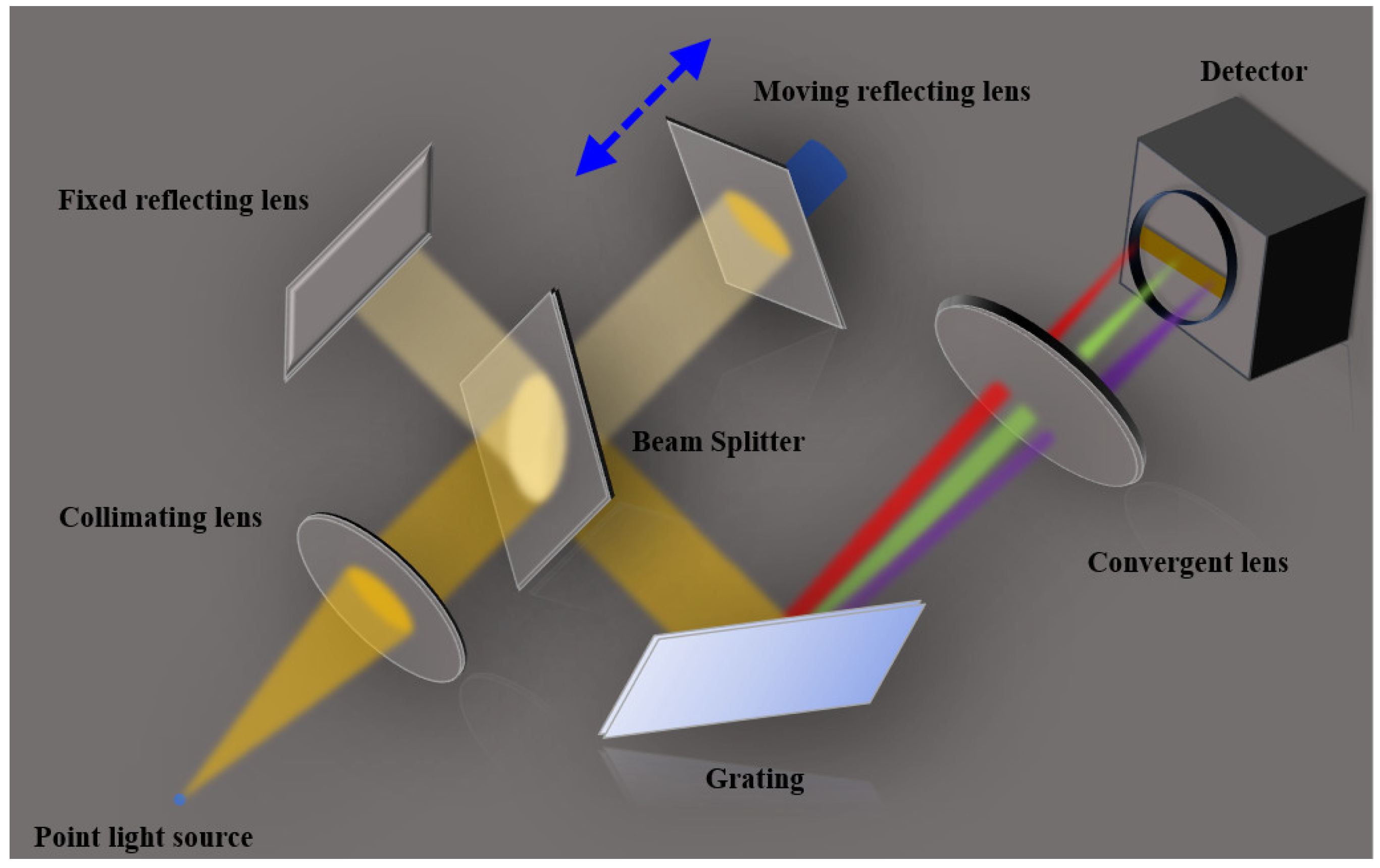
Figure 1 shows the BPS-FTS scheme based on Michelson moving mirror FTS [14], which is commonly referred to as time-modulated FTS. In this spectrometer, a grating is introduced into the interference path, dividing the broad spectrum into a sequence of narrow spectra. This allows for bandpass sampling of each interferogram corresponding to each narrowband spectrum, resulting in a substantial decrease in the number of sampling points for each interferogram. Simultaneously, bandpass sampling can widen the OPD sampling interval and reduce the sampling frequency.

While the moving mirror undergoes a uniform reciprocating motion, each pixel of the linear array sensor produces a complete interference signal corresponding to a narrowband spectrum during one-way linear motion. After applying Fourier transforms to the sampled interference signals from each pixel, a series of reconstructed narrowband spectra can be generated. These reconstructed narrowband spectra can be organized in wavenumber order, following which their intensities can be summed to obtain the spectrum for the entire range of the spectrum. 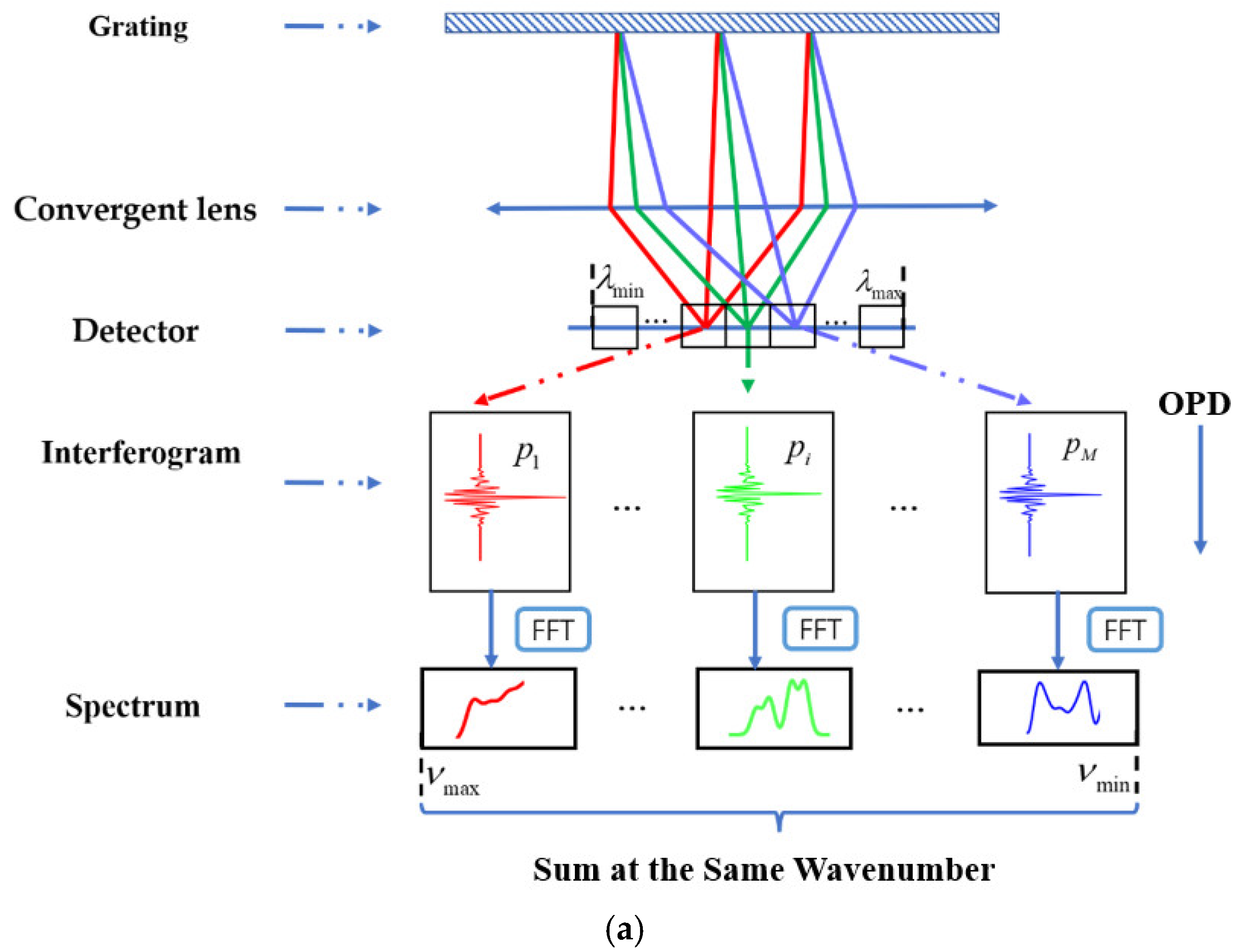Figure 2a illustrates the operating principle of BPS-FTS. Figure 2b illustrates the calculation steps of the reconstructed spectrum for each pixel.

Ideally, the diffraction effect of the grating disperses the entire spectrum detected by the sensor into a continuous distribution of monochromatic light. This monochromatic light is systematically sampled at uniform wavelength intervals by a linear array sensor, where each pixel corresponds to a specific narrow segment of the spectrum. Assuming that the range of the spectrum for pixel $j$, represented in wavenumbers, is denoted by ${\nu }_{\max }^j~{\nu }_{\min }^j$, we can apply the fundamental theory of FTS to express the interference signal received by pixel $j$, as indicated in Equation (1), with $B(\nu )$ representing the incident light intensity and $x$ representing OPD. As $x$ continuously varies within a specified range, Equation (1) allows us to generate the complete interferogram curve within a maximum OPD range.

$$I^j(x)=\frac{1}{2}{\displaystyle \underset{{\nu }_{\min }^j}{\overset{{\nu }_{\max }^j}{\int }}B\left(\nu \right)\left[1+\cos \left(2\mathsf{\pi }\nu x\right)\right]d\nu }.$$

(1)

In conventional FTS, the interferogram is typically sampled following the Nyquist sampling theorem, where the minimum frequency of the measured signal is considered to be zero. However, in practical applications, the measurable spectrum is usually limited to a finite bandwidth. Bandpass sampling theory allows the interferogram to be sampled beyond the constraints of the Nyquist sampling theorem, ensuring that the spectrum is reconstructed without introducing aliasing. Assuming incident light with a spectrum range of ${\nu }_{\min }$ to ${\nu }_{\max }$ (herein, ${\nu }_{\min }=1/{\lambda }_{\max }$ and ${\nu }_{\max }=1/{\lambda }_{\min }$), the sampling interval $\Delta x$ for the interferogram can be determined using Equation (2) [9,10,14], where $m$ is any positive integer less than or equal to ${\nu }_{\max }/({\nu }_{\max }-{\nu }_{\min })$. When $m=1$, this condition corresponds to the Nyquist sampling condition, which has been widely studied. Therefore, the theoretical analysis in this paper is limited to positive integers for $m$ within the range $[2,m_{\max }]$.

$$\frac{m-1}{2{\nu }_{\min }}\le \Delta x\le \frac{m}{2{\nu }_{\max }}.$$

(2)

Ideally, the sampled interferogram of a BPS-FTS system can be understood as the convolution of an ideal interferogram with a one-dimensional comb function. However, in practical BPS-FTS systems, in order to ensure that the sampled interferogram and the reconstructed spectrum satisfy the SNR requirement, each sampling point of the interferogram needs to be held for a short duration. Consequently, each point of the actual sampled interferogram can be considered as the integral of the product of the ideal interferogram and a rectangular function, where the width of the rectangular function corresponds to the integration time. When the spectrum reconstruction accuracy is not a concern, the rectangular sampling width can assume any value within the sampling interval $\Delta x$, as determined using Equation (1). However, when considering the spectrum reconstruction accuracy, the sampling width is usually restricted to a reasonable range. Improperly setting the sampling width can result in the distortion of the reconstructed spectrum. Therefore, it is essential to conduct a theoretical analysis to determine an effective integral sampling width that can satisfy the accuracy tolerance for spectrum reconstruction.

3. Analyzing Suitable Sampling Conditions for BPS-FTS

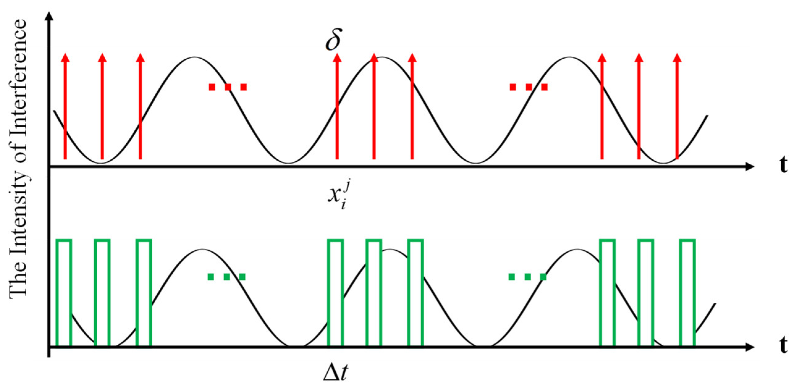
In the context of BPS-FTS, we consider that the spectrum corresponding to each pixel (denoted by $j$) is monochromatic light. In an ideal scenario, the interferogram detected by this pixel, which continuously evolves over time, takes the form of a series of cosine curves. Sampling this interferogram at perfectly equidistant intervals across the entire OPD range, assuming that the OPD corresponding to a sampling point (denoted by $i$) is $x_i^j$, yields an ideal sampling function comprising a series of impulse functions. However, practical sampling necessitates maintaining each sampling point for a certain integration time (but the OPD is still changing at this time), in order to accumulate sufficient energy and meet the signal-to-noise ratio requirements. This leads to the utilization of a rectangular sampling function. Figure 3 provides a schematic representation of monochromatic light sampling.

Assuming that the moving mirror moves at a constant speed $s$ during the sampling process and the integration time for each sampling is $\Delta t$, the corresponding change in OPD is $2s\Delta t$. The interference intensity obtained at sampling point $x_i^j$ is represented in Equation (3):

$$\begin{array}{l}I\left(x_i^j\right)=\frac{1}{2}{\displaystyle \underset{x_i^j-s\Delta t}{\overset{x_i^j+s\Delta t}{\int }}B\left(\nu \right)\cos \left(2\mathsf{\pi }\nu x\right)dx}\\ =\frac{1}{2}B\left(\nu \right)\cdot \frac{1}{\mathsf{\pi }\nu }\cos \left(2\mathsf{\pi }\nu x_i^j\right)\sin \left(2\mathsf{\pi }\nu s\Delta t\right)\\ =B\left(\nu \right)\cdot s\Delta t\cdot \cos \left(2\mathsf{\pi }\nu x_i^j\right)\mathrm{sinc}\left(2\mathsf{\pi }\nu s\Delta t\right)\end{array}.$$

(3)

Following the definition of SMTF for FTS, the SMTF corresponding to Equation (3) forms a $\mathrm{sinc}$ function. According to the SMTF criterion, it can be deduced that when the value of the SMTF decreases to within 90% of its maximum value [28,29,30], the error tolerance of the reconstructed spectrum derived from the interferogram is deemed to be acceptable. In other words, the accuracy of the reconstructed spectrum can be considered precise. In this scenario,

$$\mathrm{SMTF}=\mathrm{sinc}\left(2\mathsf{\pi }\nu s\Delta t\right)\ge 0.9.$$

(4)

In practical operations, each pixel $j$ in BPS-FTS typically corresponds to a range of the spectrum, denoted by $[{\nu }_{\min },{\nu }_{\max }]$. According to Equation (2), in this context, for any valid $m$, the corresponding range of sampling interval $\Delta x$ is $\left[\frac{m-1}{2{\nu }_{\min }},\frac{m}{2{\nu }_{\max }}\right]$. We define $d\_\Delta x$ as the range covered by this interval, which is defined as

$$d\_\Delta x=\frac{m}{2{\nu }_{\max }}-\frac{m-1}{2{\nu }_{\min }}.$$

(5)

In this case, for any $m$ that satisfies this condition, the corresponding sampling interval can be expressed as

$$\Delta x=\frac{m}{2{\nu }_{\max }}-k\cdot d\_\Delta x=\frac{\left(1-k\right)m}{2{\nu }_{\max }}+\frac{k\left(m-1\right)}{2{\nu }_{\min }},$$

(6)

where $0\le k\le 1$.

If the integration sampling time is $\Delta t$, then the sampling width of the rectangular function is $2s\Delta t=r\Delta x$($0\le r\le 1$). For any wavenumber $\nu$ within $[{\nu }_{\min },{\nu }_{\max }]$, the integrated sampling interferogram corresponding to Equation (3) can be updated using Equation (7):

$$\begin{array}{l}I\left(x_i^j\right)=B\left(\nu \right)\cdot \cos \left(2\mathsf{\pi }\nu x_i^j\right)\frac{\sin \left\{\mathsf{\pi }\nu r\left[\frac{\left(1-k\right)m}{2{\nu }_{\max }}+\frac{k\left(m-1\right)}{2{\nu }_{\min }}\right]\right\}}{2\mathsf{\pi }\nu }\\ =\frac{1}{2}B\left(\nu \right)\cdot \cos \left(2\mathsf{\pi }\nu x_i^j\right)\mathrm{sinc}\left\{\mathsf{\pi }\nu r\left[\frac{\left(1-k\right)m}{2{\nu }_{\max }}+\frac{k\left(m-1\right)}{2{\nu }_{\min }}\right]\right\}\cdot r\left[\frac{\left(1-k\right)m}{2{\nu }_{\max }}+\frac{k\left(m-1\right)}{2{\nu }_{\min }}\right]\end{array}.$$

(7)

The SMTF at this point is

$$\mathrm{SMTF}=\mathrm{sinc}\left\{\mathsf{\pi }\nu r\left[\frac{\left(1-k\right)m}{2{\nu }_{\max }}+\frac{k\left(m-1\right)}{2{\nu }_{\min }}\right]\right\}.$$

(8)

From Equation (8), it is evident that, for any wavenumber $\nu$ within the range $[{\nu }_{\min },{\nu }_{\max }]$, the SMTF associated with the integrated sampled interferogram is influenced by the values of $m$, $k$, and $r$. Different settings for these three parameters introduce variations in the SMTF, resulting in differences in the interferogram, which in turn has an impact on the reconstructed spectrum. It can be observed, from Equation (8), that when $r=p\times \frac{1}{v\left[\frac{\left(1-k\right)m}{2{\nu }_{\max }}+\frac{k\left(m-1\right)}{2{\nu }_{\min }}\right]}=p\times \frac{2{\nu }_{\max }{\nu }_{\min }}{v\left[\left(1-k\right)m{\nu }_{\min }+k\left(m-1\right){\nu }_{\max }\right]}$ (where $p$ is a non-negative integer), then $SMTF=0$. In this scenario, regardless of the variation in the OPD, a precise interferogram corresponding to the wavenumber spectrum cannot be obtained, rendering the reconstruction of the spectrum infeasible. In other words, if interferograms are obtained for different $r$ values within $0\le r\le 1$ and used for spectrum reconstruction, the resulting spectrum presents maximum distortion with a period of $T$, as shown in Equation (9).

$$T=\frac{2{\nu }_{\max }{\nu }_{\min }}{v\left[(1-k)m{\nu }_{\min }+k(m-1){\nu }_{\max }\right]}$$

(9)

Within $0\le r\le 1$, there are $N=\frac{1}{T}$ cycles, and when $m$ and $k$ are fixed, the SMTF range shifts away from its peak position and decreases rapidly as $r$ increases. The range that meets the error tolerance for spectrum reconstruction also significantly contracts. By combining Equation (4) with Equation (8), we can determine the range of $r$, as described in Equation (10):

$$r\le \frac{1}{2\nu }\cdot \frac{1}{\frac{\left(1-k\right)m}{{\nu }_{\max }}+\frac{k\left(m-1\right)}{{\nu }_{\min }}}.$$

(10)

Considering that the wavenumber range $\nu$ is constrained within $[{\nu }_{\min },{\nu }_{\max }]$, we can establish a further constraint on the values of $r$ to ensure that interferograms corresponding to all wavenumbers within the entire range of the spectrum can be accurately reconstructed within the defined error tolerance. This constraint is expressed in Equation (11):

$$r\le \frac{1}{2{\nu }_{\max }}\cdot \frac{1}{\frac{\left(1-k\right)m}{{\nu }_{\max }}+\frac{k\left(m-1\right)}{{\nu }_{\min }}}=\frac{1}{2}\cdot \frac{{\nu }_{\min }}{\left(1-k\right)m{\nu }_{\min }+k\left(m-1\right){\nu }_{\max }}.$$

(11)

Based on bandpass sampling theory, each positive integer $m$ has an associated interval that meets the SMTF criterion. For varying values of $k$ and $m$, the corresponding values of $r$ will fall within distinct intervals that satisfy the SMTF criterion constraint. When we set $r_{\lim }=\frac{1}{2}\cdot \frac{{\nu }_{\min }}{\left(1-k\right)m{\nu }_{\min }+k\left(m-1\right){\nu }_{\max }}$, accurate spectrum reconstruction becomes possible if the rectangular sampling width remains within the range of $2s\Delta t\le r_{\lim }\Delta x$, as shown in Equation (12):

$$2s\Delta t\le \frac{1}{2}\cdot \frac{{\nu }_{\min }}{\left(1-k\right)m{\nu }_{\min }+k\left(m-1\right){\nu }_{\max }}\Delta x\left(0\le k\le 1\right).$$

(12)

However, exceeding this range with the rectangular sampling width might result in the sampled interferogram failing to meet the SMTF constraint, leading to distorted reconstructed spectra. It is important to note that the aforementioned analysis explores sufficient conditions for approximate and accurate spectrum reconstruction under rectangular sampling conditions, but these cannot be considered as necessary conditions.

Further analysis revealed that, when the data are under-sampled, employing the average SMTF instead of the maximum SMTF provides a more effective means of evaluating sampling quality [31]. Given that bandpass sampling is a classic example of under-sampling, in contrast to Nyquist sampling, the SMTF criterion should be adjusted to employ the average SMTF value rather than the maximum SMTF value; specifically,

$$\left|\mathrm{SMTF}\right|\ge 0.9\overline{\mathrm{SMTF}}=0.9\overline{\mathrm{sinc}\left\{\mathsf{\pi }\nu r\left[\frac{\left(1-k\right)m}{2{\nu }_{\max }}+\frac{k\left(m-1\right)}{2{\nu }_{\min }}\right]\right\}}$$

(13)

When the value of $r$ satisfies Equation (13), the conditions for approximately accurate restoration of the spectrum can be met. Combined with the above analysis, according to the nature of the $\mathrm{sinc}$ function, since the $\mathrm{sinc}$ function has periodic zero-crossing points, then the $r$ value that meets the conditions for approximately accurate restoration of the spectrum will appear periodically in the interval confirmed by two adjacent zero-crossing points. When $\left|\mathrm{SMTF}\right|<0.9\overline{\mathrm{SMTF}}$ in a certain interval, there is no $r$ in that interval and subsequent intervals that can accurately restore the spectrum.

To establish a more suitable understanding of the relationship between the sampling integration time and the accuracy of the reconstruction of the spectrum, Chapter 4 delves into the theoretical modeling and simulation of the interferogram integration sampling process. The influence of rectangular sampling functions corresponding to various integration durations on the reconstructed spectrum is examined. A comparative analysis is conducted, aligning these results with the theoretical insights obtained in this section. This comparative analysis serves as a foundation to establish integration sampling parameters for practical systems.

4. Simulation Analysis and Verification

To assess the influence of integration sampling time on the interferogram and the resulting reconstructed spectrum, we performed the simulation using Matlab, its version number is ‘9.8.0.1873465 (R2020a) Update 8’. We used the “MATLAB and Simulink Student Suite” and “MATLAB and Simulink Student Suite” toolboxes.

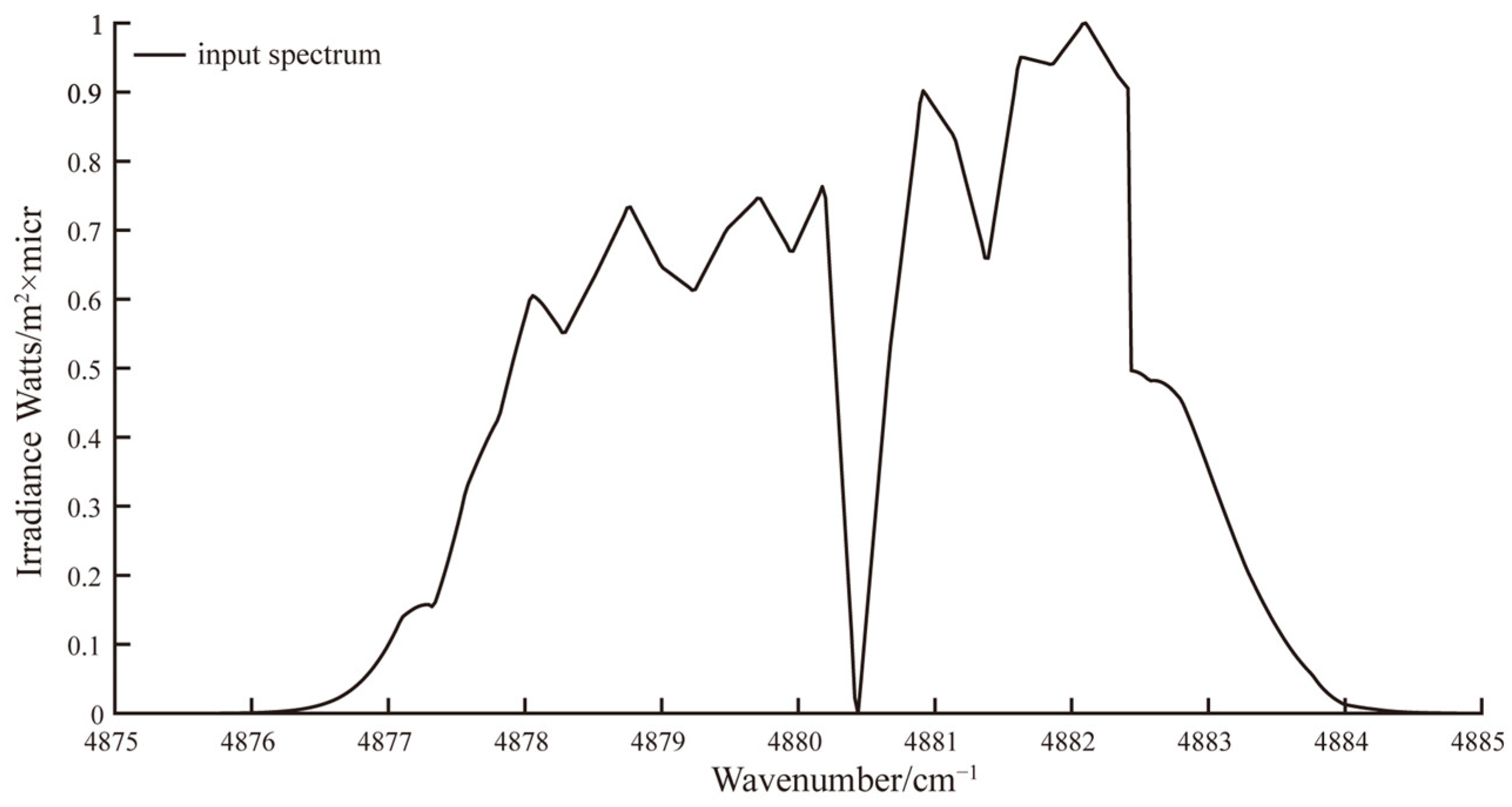
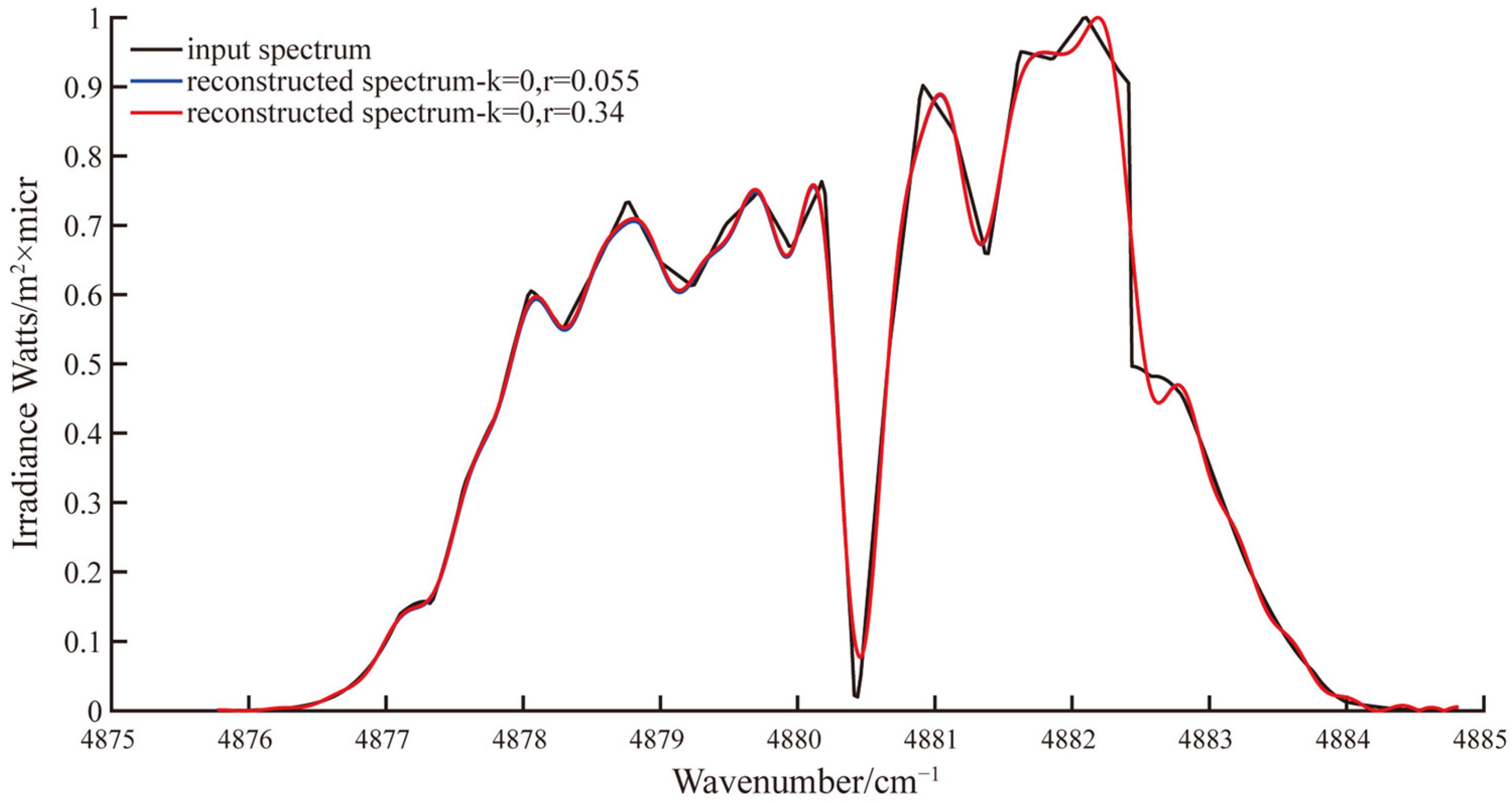
In the simulation, we refer to the standard solar spectrum and randomly select a part as the input spectrum of any pixel for analysis to ensure the randomness of the simulation analysis. This particular spectrum spanned the wavenumber range from 4875.77 cm⁻¹ to 4884.81 cm⁻¹, and its spectral profile is presented in Figure 4. In this context, in accordance with Equation (2), $m$ can assume any positive integer value up to and including 540. Without loss of generality, the simulation results of other pixels are similar to this pixel.

(1)

SMTF analysis

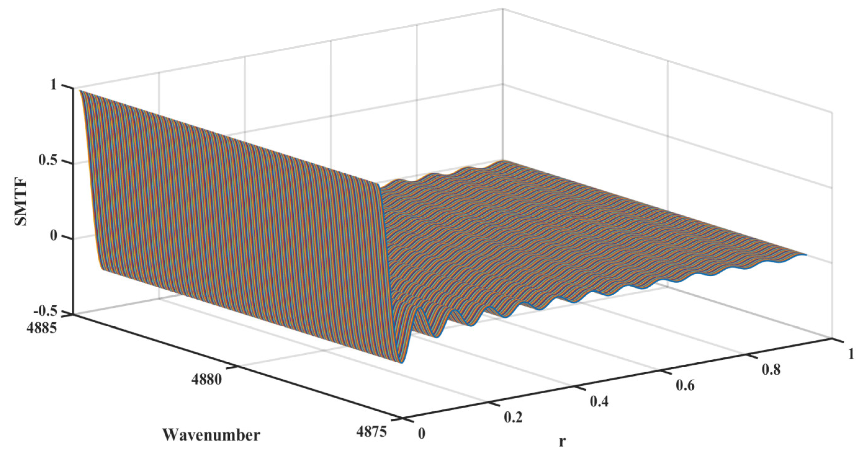
Without loss of generality, we randomly selected $m=50$ to investigate the connection between integration sampling time and SMTF under the condition $k=0$, resulting in the adjusted SMTF expression given in Equation (14):

$$\mathrm{SMTF}=\mathrm{sinc}\left\{\mathsf{\pi }\nu r\left[\frac{\left(1-k\right)m}{2{\nu }_{\max }}+\frac{k\left(m-1\right)}{2{\nu }_{\min }}\right]\right\}=\mathrm{sinc}\left(\mathsf{\pi }\nu r\frac{50}{2{\nu }_{\max }}\right).$$

(14)

SMTF curves were then generated for each wavenumber $\nu$ within the range $0\le r\le 1$, which are shown in Figure 5.

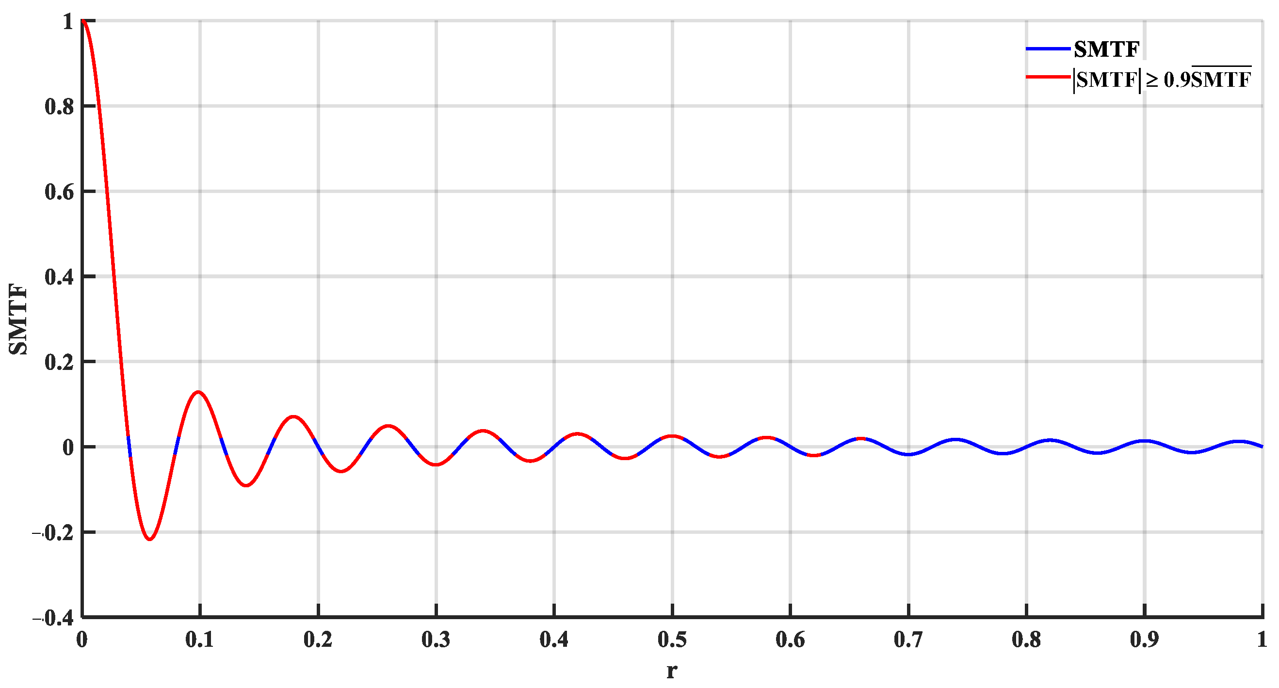
As the range of the spectrum was extremely narrow, the SMTF could be approximated using Equation (15):

$$\mathrm{SMTF}=\mathrm{sinc}\left(\mathsf{\pi }\nu r\frac{50}{2{\nu }_{\max }}\right)\approx \mathrm{sinc}⟮25\mathsf{\pi }r⟯.$$

(15)

According to the analysis in Section 3, it is apparent that, within the range of $0\le r\le 1$, the SMTF is shown in Figure 6. When Equation (13) is satisfied, the spectrum can be accurately restored. We marked the range of $r$ that satisfy this criterion in Figure 6.

From Equation (9) and Figure 5 and Figure 6, it is evident that SMTF presented zero crossings with a period of $T\approx 0.04$. This implies that significant distortion occurs in the spectrum when $r$ is an integer multiple of 0.04. In the corresponding period, some values cover the tolerance requirements of the restoration spectrum. However, as the integration time increases, because the value range that satisfies the condition of Equation (13) becomes smaller and smaller, the values of $r$ that can meet the tolerance of the restoration spectrum accuracy become smaller and smaller. Starting from the 18th interval, there will be no $r$ that can meet the restored spectrum tolerance requirements.

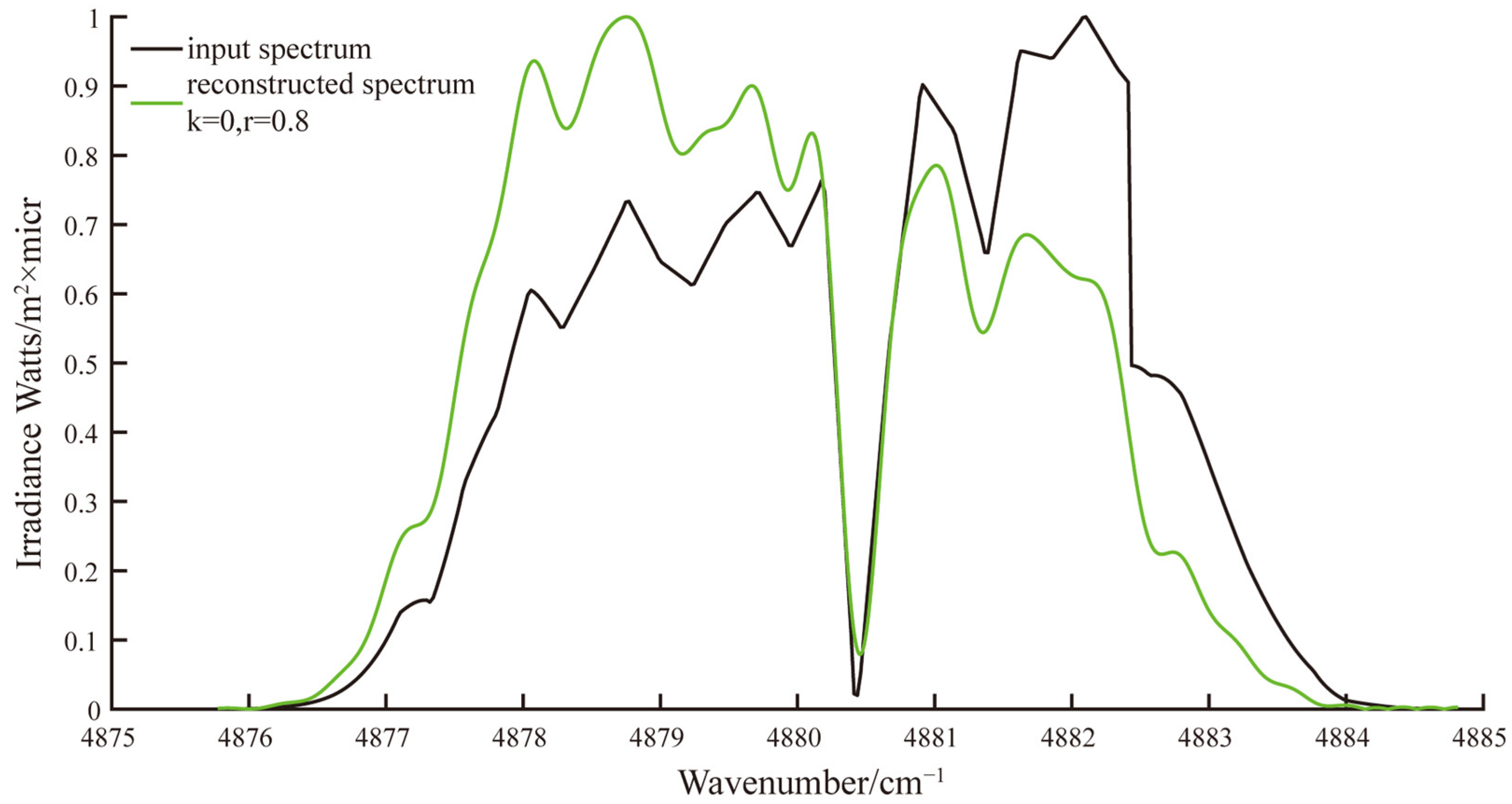
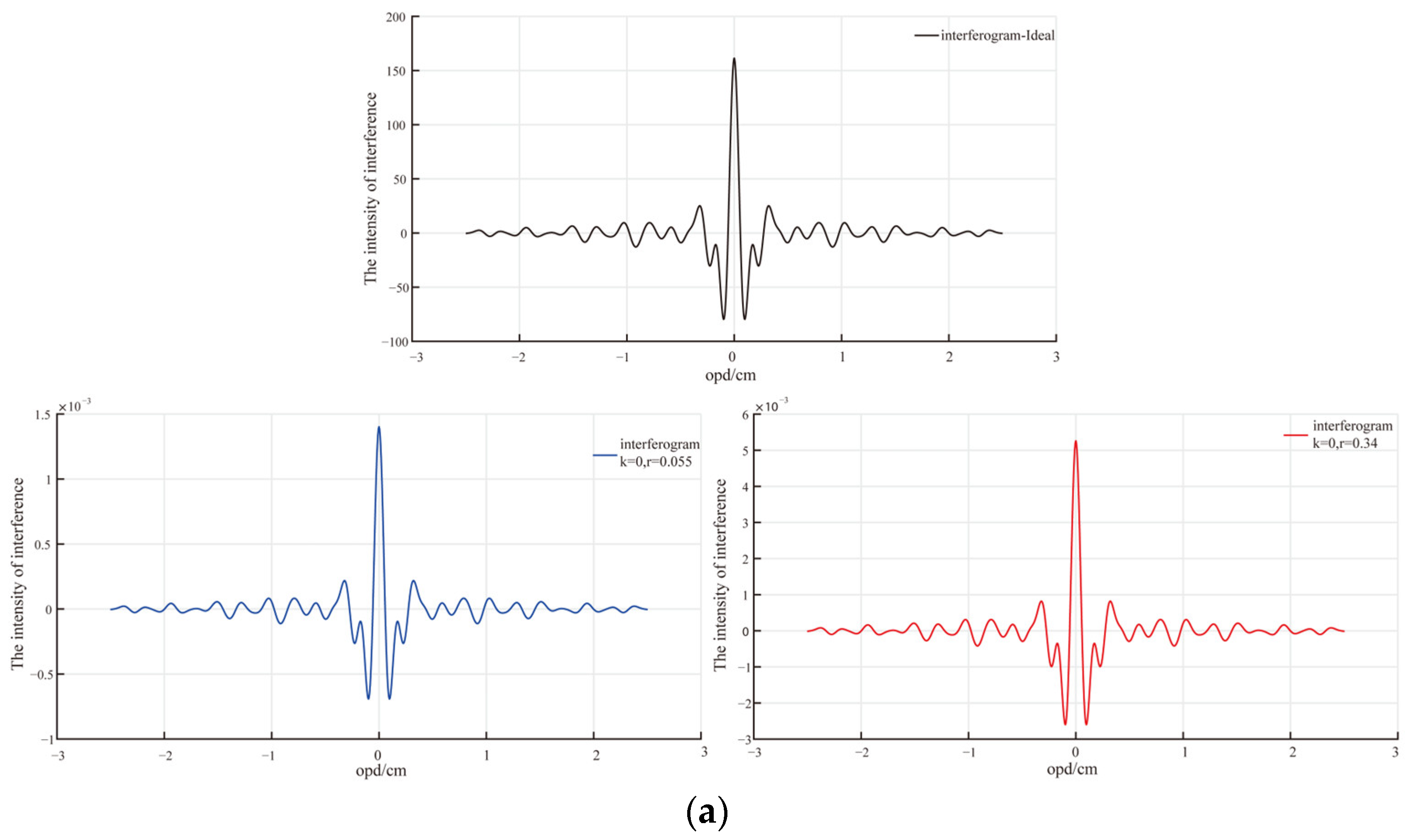
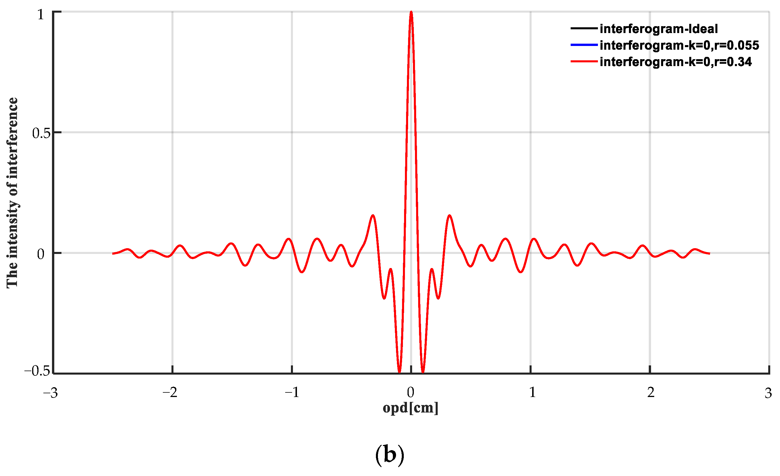
In order to verify the above conclusion, we conducted a simulation analysis of the interferogram and the reconstructed spectrum with $r=0.8=20T$. Figure 7 presents the interferogram, with a maximum OPD of 2.5 cm and a sampling interval of 0.0051 cm. The data in the figure indicate that, at this point, the interferogram error was at its maximum. Figure 8 displays the reconstructed spectrum. During spectrum reconstruction, zero-padding was applied to the interferogram to ensure the smooth display of the reconstructed spectrum curve, facilitating accurate assessment of the similarity between the reconstructed spectrum and the input spectrum. This zero-padding corresponded to data interpolation in the dimension of the reconstructed spectrum and preserved the information of the spectrum. The reconstructed spectrum clearly exhibited significant aliasing, leading to substantial distortion when compared to the shape of the input spectrum.

To quantitatively analyze the accuracy of the reconstructed spectrum, we employed the spectral relative deviation method to calculate the relative deviation between the reconstructed spectrum and the input spectrum. Additionally, the SCM method was used to assess the similarity between the reconstructed spectrum and the input spectrum, with the aim of quantitatively evaluating the accuracy of the restored spectrum under different sampling integration times [14]. Equation (16) provides the formula for calculating the relative deviation:

$$R_{error}=\frac{1}{N}{\displaystyle \sum _{n=1}^N\frac{\left|S_n^{\prime }-S_n\right|}{S_n}}\times 100\%,$$

(16)

where $S_n^{\prime }$ is the reconstructed spectrum, $S_n$ is the standard spectrum, and $N$ is the number of segments of the spectrum.

SCM is derived from the Pearson correlation coefficient, the definition of which is given in Equation (17):

$$R_{S,S^{\prime }}=\frac{{\displaystyle \sum _{n=1}^N(S_n^{\prime }-{\mu }_{S_n^{\prime }})(S_n-{\mu }_{S_n})}}{\sqrt{{\displaystyle \sum _{n=1}^N{(S_n^{\prime }-{\mu }_{S_n^{\prime }})}^2{\displaystyle \sum _{n=1}^N{(S_n-{\mu }_{S_n})}^2}}}},$$

(17)

where $S_n^{\prime }$ is the reconstructed spectrum, ${\mu }_{S_n^{\prime }}$ is the mean of the reconstructed spectrum, $S_n$ is the input spectrum, and ${\mu }_{S_n}$ is the mean of the input spectrum.

To mitigate the impact of the Gibbs effect at both ends of the spectrum on the accuracy of the reconstructed spectrum, we excluded a small portion of the data (those with relatively minor amplitudes). Calculations using Equations (16) and (17) revealed that, when $r=0.8$, the spectral relative deviation reached 39.29%, while the SCM was only 63.76%. These results demonstrate that the accuracy of the reconstructed spectrum is notably poor in this instance.

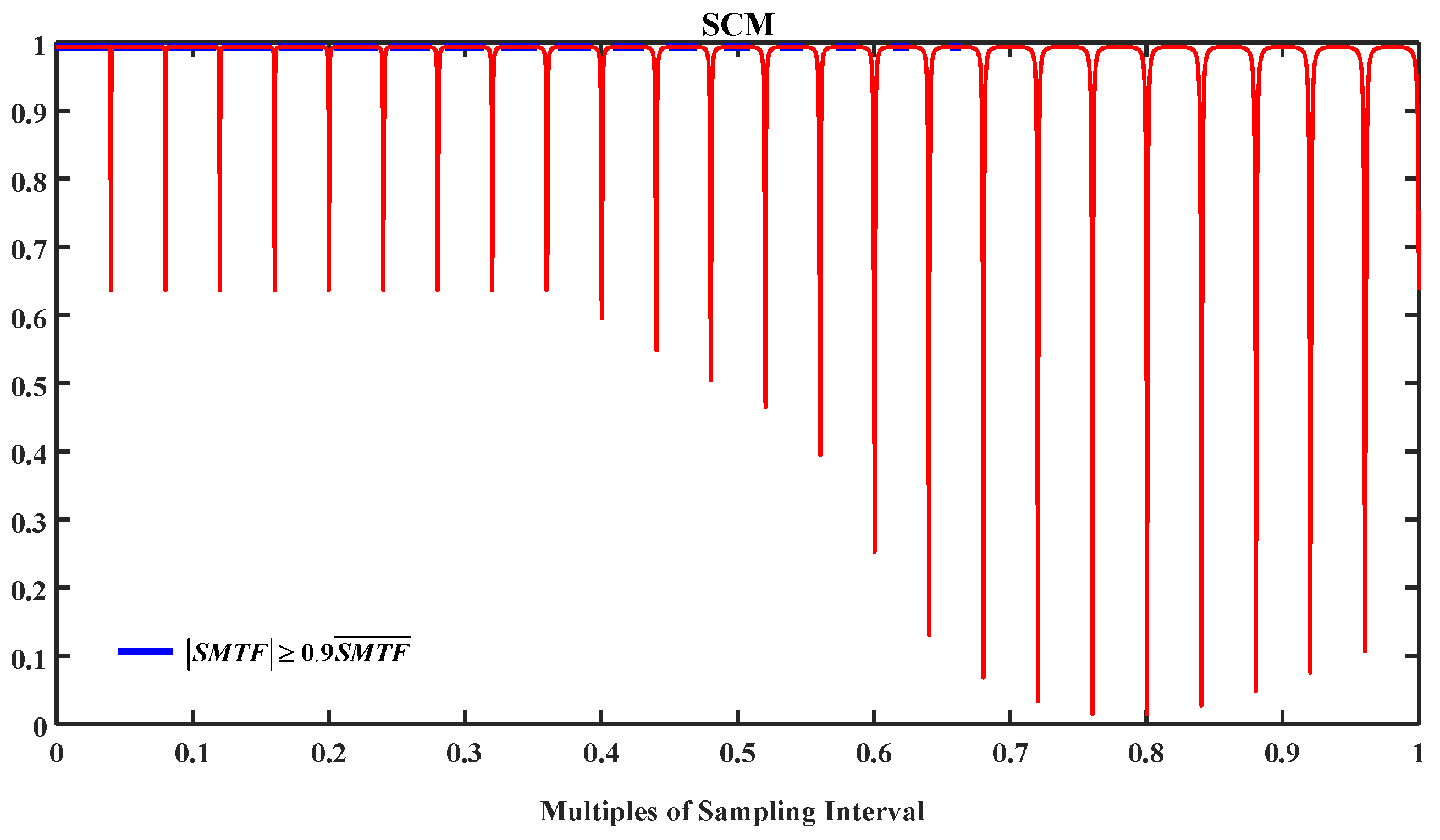
Based on the earlier analysis, it was deduced that, within the range of $0\le r\le 1$, the reconstructed spectrum exhibited significant distortion with a periodicity of $T\approx 0.04$, encompassing a total of $N=\frac{1}{T}=25$ cycles. This is corroborated by the simulation results of spectral relative deviation and SCM, depicted in Figure 9 and Figure 10. We also found that under the $r$ value marked in Figure 6, the relative spectral deviation and SCM of the corresponding restored spectrum were within the tolerance range. This also proves that the criterion of Equation (13) is more applicable to BPS-FTS than Equation (11). As $r$ increased, the spectral relative deviation generally increased, the SCM decreased, and the likelihood of reconstructed spectra distortions also increased.

(2)

Simulation Analysis of Interferograms and Reconstructed Spectra when Equation (13) is Met.

To assess the error in the reconstructed spectra when Equation (13) is met, we arbitrarily selected two values of $r$; namely, $r=0.055$ and $r=0.34$. In these two instances, we conducted simulations for interferogram sampling and the reconstruction of the spectrum based on the input spectrum. The maximum OPD of the BPS-FTS, as well as the values of $m$ and $k$, remained consistent with the parameters mentioned earlier, ensuring the same sampling interval as previously described. For these two distinct $r$ values, we derived the corresponding sampled interferograms and compared them with the ideal interferogram. The results are depicted in Figure 11. Notably, these figures reflect the $r$ values, and the normalized sampled interference data aligned closely with the ideal interference data.

After performing reconstruction of the spectrum for the two cases of $r=0.055$ and $r=0.34$, as shown in Figure 12, we observed that under these integration sampling conditions meeting Equation (13), the reconstructed spectra closely matched the original spectrum.

Table 1. Calculation results of spectral accuracy evaluation criteria.

	$\mathit{r}=0.055$	$\mathit{r}=0.34$
Spectral relative deviation	0.0556	0.0543
SCM	0.9938	0.9938

provides the calculation results for the spectral relative deviation and SCM.

From the calculation results, it is evident that, under the bandpass sampling conditions, both $r=0.055$ and $r=0.34$ yielded relatively small relative deviations in the reconstructed spectra, measuring 5.56% and 5.43%, respectively. Furthermore, the similarity between the reconstructed spectrum and the input spectrum approached one. These simulation findings indicate that, for BPS-FTS, satisfying Equation (13) allows for the reconstruction of the spectrum within the specified error tolerance range when using sampled interferograms.

5. Conclusions

The significant advantage of BPS-FTS is its ability to considerably increase the sampling interval, thereby reducing the number of required sampling points. In this paper, we conducted a comprehensive theoretical study and simulation analysis to investigate the impact of the rectangular sampling step size on the reconstructed spectrum, thus further leveraging this advantage. This research was conducted with the aim of offering valuable theoretical and technical insights for the practical implementation of this technology. In the future, we will conduct further experimental verification.

Both the theoretical analysis and simulation verification results revealed that the actual interferogram under rectangular sampling is influenced by the SMTF of FTS. In the reconstructed spectrum, this influence is evident as the product of the actual spectrum and a $\mathrm{sinc}$ function, which varies with different values of $m$. The integration time has varying effects on the reconstructed spectrum. It was observed that, when the condition shown in Equation (12) is met, the rectangular sampling step allows for accurate spectrum reconstruction within an acceptable error range. At this time, SMTF can reach 0.9. However, outside of this range, there are also some values that can meet the accuracy requirements of the constructed spectrum.

Our simulation analysis also revealed that, due to the inherent under-sampling characteristics of bandpass sampling, using the average value $\overline{\mathrm{SMTF}}$ as the MTF criterion (specifically, Equation (13)) provides a more suitable range of integration sampling times that meet the tolerance requirements of the reconstruction spectrum. Therefore, in the practical implementation of systems, Equation (13) can be considered the fundamental design and analysis criterion for integration sampling in BPS-FTS.

Our theoretical analysis further indicated that changes in integration time can cause periodic and significant distortion in the reconstructed spectrum, with a period of $T$, which is shown in Equation (9). This distortion is influenced by the values of $m$ and $k$ and becomes more pronounced as the integration time increases. It can even make the relative spectral deviation reach 39.29%, and the SCM is reduced to 63.67%. Consequently, in BPS-FTS, while it is possible to extend the sampling interval, the integration time for sampling cannot be arbitrarily increased based solely on the increased sampling interval; instead, it must adhere to the constraints mentioned earlier. This also confirms the correctness of Equation (13) from another aspect.