SocialJGCF: Social Recommendation with Jacobi Polynomial-Based Graph Collaborative Filtering

Abstract

With the flourishing of social media platforms, data in social networks, especially user-generated content, are growing rapidly, which makes it hard for users to select relevant content from the overloaded data. Recommender systems are thus developed to filter user-relevant content for better user experiences and also the commercial needs of social platform providers. Graph neural networks have been widely applied in recommender systems for better recommendation based on past interactions between users and corresponding items due to the graph structure of social data. Users might also be influenced by their social connections, which is the focus of social recommendation. Most works on recommendation systems try to obtain better representations of user embeddings and item embeddings. Compared with recommendation systems only focusing on interaction graphs, social recommendation has an additional task of combining user embedding from the social graph and interaction graph. This paper proposes a new method called SocialJGCF to address these problems, which applies Jacobi-Polynomial-Based Graph Collaborative Filtering (JGCF) to the propagation of the interaction graph and social graph, and a graph fusion is used to combine the user embeddings from the interaction graph and social graph. Experiments are conducted on two real-world datasets, epinions and LastFM. The result shows that SocialJGCF has great potential in social recommendation, especially for cold-start problems.

1. Introduction

In the age of information explosion, users need tools to accurately filter personally relevant information from the noisy data [1]. A recommender system is a powerful decision-making tool for users that addresses the information overload problem and has been widely applied in online services, e.g., e-commerce platforms (Amazon, BestBuy), and social platforms (X, Facebook). Recommender systems aim to provide lists of items that users will likely interact with (e.g., click or purchase) [2,3]. Traditionally, recommender systems use collaborative filtering to extract effective user patterns and item patterns from past user–item interaction data. However, there remains a significant research gap in effectively utilizing the rich information available in social networks to improve the accuracy and personalization of recommendations, especially for new users or items with limited interaction history.

Psychology [4] and life experiences show that people tend to have similar preferences within their social relationships and tend to be easily influenced by them. It indicates that a user’s connections might provide additional assistance in deciding the preference of the user, and information about social relationships might enhance the performance of recommender systems if properly integrated. Recently, studies [5,6] have realized the potential influence of social relationships in recommender systems. In the case where the recommender system utilizes users’ social information for better recommendation performance, the system is called a social recommender system.

By modeling users and items as nodes, and their interactions and social connections as edges, we can represent the user–item interaction data and social data using a user–item interaction graph and a social graph [7,8]. Obviously, both graphs contain user information, and, to build reliable social recommendation systems, we need to extract and integrate user information from both [9,10]. Generally, two frameworks can be adopted to compute the integrated representation [9]: bipartite graph strategy, where the two graphs are first propagated separately and the final user representations are computed later [7,11,12], and unified graph strategy, where the two graphs are combined into one graph and the final representation is obtained by propagating the unified graph [13,14].

In recent years, graph neural networks (GNNs), which were proposed to effectively learn node representations and obtain meaningful information from graphs, have been widely applied in graph-structured data [15,16,17,18]. The core of GNNs lies in their ability to propagate node information through the network via node connections, allowing for the integration of local neighborhood features into the learning process. This capability enables GNNs to generalize and infer node and graph properties dynamically, thus addressing tasks that involve complex graph data more effectively than traditional neural network models.

Due to the superiority of GNNs for graph data, GNNs have been widely applied in recommender systems [19,20,21,22,23], especially social recommendation systems [6,24,25]. Compared with previous non-GNN-based methods, GNN-based social recommendation methods have achieved better recommendation accuracy on real-world datasets.

The paper proposes a new GNN-based social recommendation system called SocialJGCF. SocialJGCF adopts the bipartite graph approach, and the final user representation is an adaptive weighted average of the user representation from the interaction graph and social graph, while final item representation is computed by the propagation of the user–item interaction graph.

The paper is structured as follows: Section 2 summarizes related work on recommendation systems. Section 3 gives a basic notation of the social recommendation problem and JGCF and presents the design of the SocialJGCF algorithm. Section 4 analyzes the experiment results of the proposed SocialJGCF. Section 5 concludes the paper.

2. Problem and Related Work

2.1. Problem Statement

Recommendation problems focus on analyzing users’ interest in specific items from their past interactions with items. These interactions can be either quantified explicitly by ratings given by users (e.g., like and dislike for YouTube videos or stars in Amazon customer reviews) or only shown implicitly (e.g., users’ clicks on some products on Amazon). In the former case, the rating matrix can be used to represent user–item interaction, and, in the latter case, the implicit feedback data can be converted to explicit ratings.

Recently, many methods have been proposed for recommender systems based on user–item interaction graphs [19,20,26,27,28,29,30]. LightGCN simplifies graph convolution by only including neighborhood aggregation [19]. Simple Graph Contrastive Learning (SimGCL) combines contrastive learning with LightGCN to mitigate popularity bias [26]. Jacobi-Polynomial-Based Graph Collaborative Filtering (JGCF) uses Jacobi polynomial bases to approximate a LightGCN-based filter from a spectral transformation view [27].

However, practically, each user only interacts with a small subset of available items, which results in a highly sparse rating matrix, making the recommendation problem hard to solve. One common strategy to mitigate the data sparsity problem is to enrich the representation by the integration of supplementary information such as item–item relationships and user–user relationships. In many open datasets, relationships between items are not explicitly defined, but rather inferred from their co-occurrence in previous interactions [9,31]. This method of constructing relationships can compromise the effectiveness of the recommender system if not thoughtfully implemented. Conversely, the user–user relationship data are readily accessible due to the growth of social media platforms.

Social influence theory indicates that people are likely to be influenced by their connections and perform similar actions. Therefore, users’ social relationships can be incorporated into recommendation systems to enhance performance, which is the focus of social recommendation problems.

Cold-start problems are a critical challenge in recommender systems, where new users or items have a limited interaction history, making prediction difficult. This issue is further exacerbated in social recommendation systems, which need to integrate user information from both the interaction and social graphs.

Formally, the graph-based social recommendation problem can be expressed as follows: The user set and item set are denoted, respectively, as $U$ and $I$, where $\left|U\right|=N$ and $\left|I\right|=M$. The social recommendation problem usually involves two graphs, the user–item interaction graph and the social graph. The user–item interaction graph is defined as $\left\{\left(u,i,y_{ui}\right)|u\in U, i\in I, y_{ui}\ge 0\right\}$, where $y_{ui}$ is the edge weight between user $u$ and item $i$, and $y_{ui}=0$ indicates there is no interaction between them. The interaction graph can be represented as an adjacency matrix ${\widehat{A}}_{UI}\in R^{\left(N+M\right)\times \left(N+M\right)}$. The social graph is denoted as $\left\{\left(u_i, u_j, s_{ij}\right)|u_i, u_j\in U, s_{ij}\in \left\{\mathrm{0,1}\right\}\right\}$, where $s_{ij}=1$ if user $u_i$ and user $u_j$ have a social connection. The adjacency matrix of the social graph is denoted as ${\widehat{A}}_S$.

2.2. Related Work

Due to the emergence of social networks, it is recognized that the user representation can be enhanced if the local neighbors of each user are considered [8,9,32]. Social recommendation systems have two main issues: the degree of influence by friends, which is also called social trust, and many trust-based methods have been proposed to infer trustworthy values for recommendation [33,34,35,36], and user representation integration [9]. The trustworthy values between users and their connections indicate the degree of social influence. Many trust-based methods have been proposed to incorporate social trust into the recommendation system for better performance. DiffNet [7] assumes friends have equal influence by using mean-pooling. ESRF [5] adopts an autoencoder mechanism to filter unreliable social connections to improve recommendation accuracy.

Normally, social recommendation systems involve two graphs, the user–item interaction graph and the social graph. Since both of them contain user representations, multiple methods have been proposed for combining user representation from the social graph and from the interaction graph, either creating a unified graph from these two graphs or simply fusing user representations from the two separate graphs.

Unified graph approaches merge the social graph and interaction graph together and apply graph learning methods to the unified graph to learn node embeddings. DiffNet++ [13] captures both social influence and user interest in a unified graph and applies graph attention and diffusion layers to learn the final representations. HeteroGraphRec [37] treats the users and items as different types of nodes and social interactions and user–item interactions as different types of edges. Then, the social recommendation problem can be solved by learning representations from the heterogeneous graph.

Compared with the unified graph approach, the dual graph approach is more flexible, since we can use different propagation depths for the two graphs and different models can be applied to the two graphs for better performance. DGRec [38] applied a graph attention network on the social graph which captures multi-hop social influences, and applied gated recurrent units on the user–item interaction sequences to capture the sequential patterns in user behavior. STGCN [39] uses graph convolution on the social graph to pretrain the user representations, which are then fine-tuned on the user–item interaction graph. For some dual graph approaches, the user representations from the social graph and user–item interaction graph should be effectively fused. In addition to the attention mechanism used in DGRec [38], a multi-layer perceptron can also be applied to the concatenated embedding vector to fuse the two representations [11,40,41,42]. To effectively develop effective social recommendation systems which take the separate graph approach, the authors of [41] considered the co-occurrence frequency of item attributes to augment item embeddings. Despite the effectiveness of these methods, social recommendation systems still suffer in cold-start scenarios, where no or only a few interactions exist for a new user or item [24,33,40]. The comparisons with other papers are summarized in

Table 1. Comparisons with other papers.

	Unified Graph	Dual Graphs
		Non-Frequency Based	Frequency Based
Trust-based recommendation	[7,13,37]	[11,38,39,42]	[41]
Cold-start recommendation	[24]	[40]	this paper

.

3. Method

3.1. Overall Architecture

The overall architecture of SocialJGCF is depicted in Figure 1a. The system consists of 3 parts: the initial embedding layer, propagation layer, and prediction layer. As shown in Figure 1, any user $u$ in the social graph and the user in the interaction graph are represented as vectors in the embedding layer, and any item $i$ interacted with by user $u$ in the user–item interaction graph is also embedded into a vector. Details of the embedding layer are explained in Section 3.1.1. Then, the representations from the social graph and interaction graph in the embedding layer are fed separately into the propagation layer, which we will cover in Section 3.1.2. Finally, in the prediction layer, the user embeddings from the two graphs are combined and the prediction is made by using the final user embedding and the item embedding. The prediction layer is explained in Section 3.1.3.

3.1.1. Embedding Layer

In typical datasets, labels are used to represent both users and items. The data showing interactions and social connections are typically formatted as pairs of these labels. Our method requires numeric values for computation, so these non-numeric labels should be transformed into vector representations. The conversion is handled by the embedding layer in Figure 1a. For nodes in the user–item interaction graph, the initial embedding layer encodes any user u (or item i) with vector $e_u^{\left(0\right)}\in R^d\left(e_i^{\left(0\right)}\in R^d\right)$, where $d$ is the predefined embedding size. The superscript $\left(k\right)$ indicates the embeddings, and $e_u^{\left(k\right)}\left(e_i^{\left(k\right)}\right)$ are the outputs of the $k$th propagation layer. The initial embeddings $e_u^{\left(0\right)}$ and $e_i^{\left(0\right)}$ follow a random distribution. Suppose the dataset contains $N$ users and $M$ items. The embedding of all users(items) can be represented as $E_U^{\left(0\right)}\in R^{N\times d}$ ($E_I^{\left(0\right)}\in R^{M\times d})$, whose $u$th ($i$th) row is the transpose of the embedding of user $u$(item $i$). Similarly, in the social graph, the initial embedding layer encodes any user $u$ into an arbitrary vector $e_s^{\left(0\right)}\in R^d$, and the embeddings of all users in the social graph can be represented as $E_S^{\left(0\right)}\in R^{N\times d}$.

3.1.2. Propagation Layer

Essentially, the task of recommendation systems is to predict possible future user–item interactions given past interactions. This can be mathematically formulated as finding a map $f$ from past interactions $A\in R^{N\times N}$ to future interactions $A^{\prime }\in R^{N\times N}$. $A$ and $F$ are adjacency matrices where $A_{ij}=1$ indicates user $i$ had past interactions with item $j$ and ${A^{\prime }}_{ij}=1$ indicates user $i$ probably will interact with item $j$ in the future. Formally, the optimization of the recommender system can be denoted as

$$\min \left|\right|f\left(A\right)-A\prime |\hspace{0.5em}{|}_F,$$

where $\left|\right|\cdot |\hspace{0.5em}{|}_F$ is the Frobenius norm. Since $A$ is a symmetric matrix, we can perform eigen decomposition on it, $A=Q\mathsf{\Lambda }{Q}^T$, where $Q\in R^{N\times N}$ is an orthonormal matrix whose columns are eigenvectors of $A$, and $\mathsf{\Lambda }\in R^{N\times N}$ is a diagonal matrix containing all the eigenvalues of $A$. Considering the invariance property of the Frobenius norm under orthonormal projection, we can restate the objective as

$$\begin{array}{c}\min \left|\right|f\left(A\right)-A\prime |\hspace{0.5em}{|}_F=\min \left|\right|f\left(Q\mathsf{\Lambda }{Q}^T\right)-A\prime |\hspace{0.5em}{|}_F\hfill \\ =\min \left|\right|Qf\left(\mathsf{\Lambda }\right)Q^T-A\prime |\hspace{0.5em}{|}_F\hfill \\ =\min \left|\right|f\left(\mathsf{\Lambda }\right)-Q^{T}A\prime Q|\hspace{0.5em}{|}_F.\hfill \end{array}$$

While the equation is still difficult to optimize directly, we can observe that the optimization is towards function $f$ and the off-diagonal elements of $f\left(\mathsf{\Lambda }\right)$ do not contribute to the Frobenius norm. Then, the objective can be simplified to an equivalent least-square fitting objective,

$$\min \sum _i{\left(f\left({\mathsf{\Lambda }}_{ii}\right)-Q_{\cdot i}^T{A}^{\prime }{Q}_{\cdot i}\right)}^2,$$

which shows that a good mapping function $f$ should extract the relationship of $\mathsf{\Lambda }$ and the diagonals of $Q^{T}A\prime Q$.

Generally, the propagation layer captures higher-order connections between users and items within the user–item interaction graph and relationships between users in the social graph. LightGCN [19] is a popular method for propagation layers due to its simplicity, and takes the form

$$E^{\left(K\right)}={\displaystyle \frac{1}{K+1}}\sum _{k=0}^K{E}^{\left(k\right)}=\sum _{k=0}^K{\displaystyle \frac{{\widehat{A}}^{\left(k\right)}}{K+1}}{E}^{\left(0\right)}.$$

The formula suggests that the final embedding $E^{\left(K\right)}$ is derived by applying the filter ${\displaystyle \sum _{k=0}^K}{\widehat{A}}^{\left(k\right)}$ to the initial embedding $E^{\left(0\right)}$. However, the bases of the filter are not orthogonal to each other, lacking mutual independence, and thus their ability to extract essential information in the final embedding is limited.

A Jacobi polynomial is an orthogonal and expressive basis which is widely used in scientific computations. This makes it an appropriate alternative to LightGCN, which is the core of JGCF and is the main method in the propagation layer. JGCF takes a spectral view of the recommendation task, and finds the correlation of the interaction signal frequency between the training data and the test data [27]. Thus, JGCF designs a frequency filter for the recommendation task and applies Jacobi polynomials to estimate the filter. Since the signals with low frequency or high frequency in training data show a strong linear correlation with that in test data, no activation is applied and the propagation formula is

$$E_{band-stop}^{\left(K\right)}={\displaystyle \frac{1}{K+1}}\sum P_k^{a,b}\left(\widehat{A}\right)E^{\left(0\right)}.$$

Here, $P_k^{a,b}$ represents the Jacobi polynomial of order k with parameters a and b. These parameters influence the filter’s frequency response, allowing for control over which frequency bands are emphasized or attenuated.

For mid-frequency signals, JGCF takes a typical design in the spectral GNN and the band-pass filter is given by

$$E_{band-pass}^{\left(K\right)}=\mathrm{t}\mathrm{a}\mathrm{n}\mathrm{h}\left(\left(\mathsf{\alpha }\mathrm{I}-{\displaystyle \frac{1}{K+1}}\sum P_k^{a,b}\left(\widehat{A}\right)\right)E^{\left(0\right)}\right).$$

To give an accurate recommendation prediction for a user, both the band-stop and band-pass should be used, and the final representation is given by their concatenation:

$$E=\left[E_{band-stop}^{\left(K\right)}; E_{band-pass}^{\left(K\right)}\right]$$

For the propagation of embeddings, JGCF is applied to the social graph and user–item interaction graph independently. The final output embedding of the user–item interaction graph $E_{UI}\in R^{\left(N+M\right)\times 2d}$ is given by the concatenation of two embeddings, $E_{band-stop}^{\left(K\right)}$ and $E_{band-pass}^{\left(K\right)}$, where

$$E_{band-stop}^{\left(K\right)}={\displaystyle \frac{1}{K+1}}\sum P_k^{a,b}\left(\widehat{A}\right)E^{\left(0\right)}, E^{\left(0\right)}\in R^{\left(N+M\right)\times d}=\left[E_U^{\left(0\right)};E_I^{\left(0\right)}\right]$$

and

$$E_{band-pass}^{\left(K\right)}=\mathrm{t}\mathrm{a}\mathrm{n}\mathrm{h}\left(\left(\mathsf{\alpha }\mathrm{I}-{\displaystyle \frac{1}{K+1}}\sum P_k^{a,b}\left(\widehat{A}\right)\right)E^{\left(0\right)}\right)$$

The output embedding of social graph $E_S\in R^{N\times 2d}$ is similar to $E_{UI}$, except that $E^{\left(0\right)}$ is simply $E_U^{\left(0\right)}$ and $\widehat{A}$ is the adjacency matrix of the social graph. Finally, $E_{UI}$ and the user embedding $E_{Uf}\in R^{N\times 2d}$ from $E_{UI}$ and $E_S$ are combined together to form the final user embedding $E_U$:

$$E_U=\beta E_S+\left(1-\beta \right)E_{Uf}$$

where $\beta \in \left(\mathrm{0,1}\right)$ can be either predefined or trained with the model.

3.1.3. Prediction Layer

Then, the prediction can be made by using the final user embedding from the output propagation layers and the final item embedding is contained in $E_{UI}$. The interest score of user $u$ for item $i$ is given by the inner product of their final embeddings:

$$y_{ui}=e_u^T{e}_i$$

Here, $e_u^T$ and $e_i$ are indeed vectors. They represent the final user embedding and item embedding, respectively. In addition, it is not necessary to have the same number of users and items.

3.2. Complexity Analysis

In this section, we analyze the time complexity and space complexity of SocialJGCF. The pseudocode for SocialJGCF is presented in Algorithms 1 and 2.

Algorithm 1 SocialJGCF

1: Procedure SocialJGCF (${\widehat{A}}_S,{\widehat{A}}_{UI}$)     Input: $\hspace{0.5em}\hspace{0.5em}\hspace{0.5em}\hspace{0.5em}\hspace{0.5em} {\widehat{A}}_S$—adjacency matrix of social graph $\hspace{0.5em}\hspace{0.5em}\hspace{0.5em}\hspace{0.5em}\hspace{0.5em} {\widehat{A}}_{UI}$—adjacency matrix of user-item interaction graph 2:        Initialize:$E_S^{\left(0\right)},E_U^{\left(0\right)},E_I^{\left(0\right)}\leftarrow$ initial embeddings for users and iterms 3:        $E_{UI}^{\left(0\right)}\leftarrow \mathrm{C}\mathrm{O}\mathrm{N}\mathrm{C}\mathrm{A}\mathrm{T}(E_U^{\left(0\right)},E_I^{\left(0\right)})$ 4:        $E_S^{\left(K\right)}\leftarrow \mathrm{J}\mathrm{G}\mathrm{C}\mathrm{F}(E_S^{\left(0\right)},{\widehat{A}}_S)$ 5:        $E_{UI}^{\left(K\right)}\leftarrow \mathrm{J}\mathrm{G}\mathrm{C}\mathrm{F}(E_{UI}^{\left(0\right)},{\widehat{A}}_{UI})$ 6:        $E_U^{\left(K\right)},E_I^{\left(K\right)}\leftarrow \mathrm{S}\mathrm{P}\mathrm{L}\mathrm{I}\mathrm{T}\left(E_{UI}^{\left(K\right)}\right)$ 7:        $E_U^{\left(K\right)}\leftarrow \mathsf{\beta }{E}_S^{\left(K\right)}+(1-\mathsf{\beta })E_U^{\left(K\right)}$ 8:        return$E_U^{\left(K\right)},E_I^{\left(K\right)}$ 9: end procedure

Algorithm 2 JGCF

1: Procedure JGCF ($E,\widehat{A}$) 2:       Initialize:$P_0^{a,b}\left(\widehat{A}\right)\leftarrow$I 3:       Initialize:$P_1^{a,b}(\widehat{A})\leftarrow {\displaystyle \frac{a-b}{2}}$$+{\displaystyle \frac{a+b+2}{2}}\widehat{A}$ 4:       for$k\leftarrow 1$ to K do 5:          $P_k^{a,b}\left(\widehat{A}\right)\leftarrow {{\theta }_{K}P}_{k-1}^{a,b}\left(\widehat{A}\right)+{{\theta }_K^{‘}P}_{k-1}^{a,b}\left(\widehat{A}\right)-{\theta }_K^{‘’}{P}_{k-2}^{a,b}\left(\widehat{A}\right)$ 6:       end for 7:       $E_{band-stop}\leftarrow {{\displaystyle \frac{1}{K+1}}P}_k^{a,b}\left(\widehat{A}\right)E$ 8:        $E_{band-pass}\leftarrow \mathrm{t}\mathrm{a}\mathrm{n}\mathrm{h}(\alpha E-E_{band-stop})$ 9:       $E^{\left(K\right)}\leftarrow \mathrm{C}\mathrm{O}\mathrm{N}\mathrm{C}\mathrm{A}\mathrm{T}(E_{band-stop},E_{band-pass})$ 10:       return$E^{\left(K\right)}$ 11: end procedure

3.2.1. Time Complexity

Given edge set $E$ and total number of nodes $n$, the time complexity for JGCF is $O\left(d\left(n+K\left|E\right|\right)\right)$, where $d$ is the embedding dimension and $K$ is the order of the Jacobian polynomial [27]. In SocialJGCF, JGCF is applied both in the social graph and the user–item interaction graph. Thus, the time complexity for graph convolution in SocialJGCF is $O\left(d\left(2N+M+K\left(\left|E_{UI}\right|+\left|E_S\right|\right)\right)\right)$, where $N,M,E_{UI},E_S$ are the number of users, number of items, edge set for the user–item interaction graph, and edge set for the social graph, respectively.

3.2.2. Space Complexity

The trainable parameters in SocialJGCF are mainly the initial embeddings for users and items, i.e., $E_S^{\left(0\right)},E_U^{\left(0\right)},E_I^{\left(0\right)}$, which, in total, take approximately $\left(2N+M\right)d$ of storage, which is common in embedding-based models such as LightGCN [19]. Additionally, SocialJGCF also contains other parameters such as the recurrent coefficient in the Jacobian polynomial and the learnable parameters when combining the user embeddings, but they only take constant space. This shows that the space complexity of SocialJGCF is reasonable.

4. Experiments

4.1. Experimental Setup

The experiments are conducted on two real-world datasets, LastFM and epinions. LastFM is a music-related dataset and contains information about the social network between users and their interactions with items. Epinions is a shopping dataset which also contains the trust network between users. Compared with ciao, used in SocialLGN [40], epinions is significantly sparser and more challenging, thus making it more suitable for comparing the performance of algorithms. The statistics of the two datasets are in

Table 2. Statistics of the two datasets.

Dataset	LastFM	Epinions
User #	1892	22,164
Item #	17,632	296,277
Interaction #	92,834	922,267
Interaction Density	0.278%	0.140%
Relation #	25,434	355,494
Relation Density	0.711%	0.072%

.

For each dataset, 80% of the interaction data are randomly selected for the training set, and the rest are used as the test set. Moreover, 10% of the training set is used as the validation data.

SocialJGCF is compared with recent recommender system baselines. The baselines are listed below:

• BPR [43]: a classical matrix factorization method.
• LightGCN [19]: a graph-based model which simplifies graph convolution operations for recommender systems.
• SocialLGN [40]: a LightGCN-based social recommendation model which combines social information and interaction data.

In this paper, three commonly used metrics, precision, recall, and Normalized Discounted Cumulative Gain (NDCG), are used to evaluate the top-K recommendation. The precision metric is the ratio of the recommendation list in the real record,

$$Precision@K={\displaystyle \frac{\sum l_{rec}^u\cap R_u}{N}},$$

where $l_{rec}^u$ is the top-N recommendation list of user $u$ and $R_u$ represents the set of items that user $u$ interacted with in the dataset. The recall is the percentage of how many user–item records are included in the final recommendation list.

$$Recall@K={\displaystyle \frac{\sum l_{rec}^u\cap R_u}{\sum R_u}}.$$

NDCG describes the accuracy of the recommendation list, and is computed as the average of all users’ NDCG:

$$NDCG@K\left(u\right)={\displaystyle \frac{DCG\left(u\right)}{IDCG\left(u\right)}},$$

$$DCG\left(u\right)=\sum {\displaystyle \frac{2^{re{l}_j}-1}{{\log }_2\left(j+1\right)}},$$

where $re{l}_j$ is the relevance score of the item at position $j$ and $re{l}_j=1$ only when the $jth$ item in the recommendation list is adopted by the user. The IDCG, the ideal discounted cumulative gain, is the best possible DCG that could be achieved if all items were ranked in the perfect order of relevance. Moreover, a full-ranking strategy is adopted, and all the items are ranked. This paper reports the performance with $K=10, 20$.

In this paper, we optimize the model parameters $E_S^{\left(0\right)},E_U^{\left(0\right)},E_I^{\left(0\right)}$, which are the initial embedding for users in the social graph and the users and items in the user–item interaction graph, respectively, by minimizing the Bayesian Personalized Ranking (BPR) loss [43]:

$$L_{BPR}=\sum -\ln \left(y_{ui}-y_{uj}\right)+\lambda {\left|\left|E^{\left(0\right)}\right|\right|}^2,$$

where $E^{\left(0\right)}$ is the initial embeddings of all users and all items from the embedding layer. The BPR loss encourages the recommender system to assign a higher ranking score to those interaction pairs that already exist in the dataset than to those that do not exist in the dataset.

SocialJGCF is implemented based on the SocialLGN repository using PyTorch 2.5. All the models are optimized using Adam with a 1 × 10⁻³ learning rate and the hyperparameters of the baseline models are chosen according to the suggestion in their papers. The embedding size is set to be 64. The number of propagation layers $K=3$. The experiments are conducted on an RTX 4090 GPU (NVIDIA, Santa Clara, CA, USA).

4.2. Performance Evaluation

The performance of SocialJGCF is evaluated on the LastFM and epinions dataset and comparison is made between SocialJGCF and other baseline models. Its performance on cold-start datasets is also investigated. The cold-start definition is the same as the definition in the SocialLGN paper [40].

Table 3. Comparison between SocialJGCF and other baselines on original LastFM and epinions dataset.

Dataset	Metric	BPR	LightGCN	SocialLGN	SocialJGCF	Improvement
LastFM	Precision@10	0.1449	0.1960	0.1972	0.1997	1.2677%
	Precision@20	0.1062	0.1359	0.1368	0.1380	0.8772%
	Recall@10	0.1480	0.2003	0.2026	0.2036	0.4936%
	Recall@20	0.2177	0.2771	0.2794	0.2815	0.7516%
	NDCG@10	0.1835	0.2536	0.2566	0.2575	0.3507%
	NDCG@20	0.2095	0.2789	0.2822	0.2832	0.3543%
Epinions	Precision@10	0.0184	0.0228	0.0215	0.0221	2.7907%
	Precision@20	0.0149	0.0184	0.0175	0.0183	4.5714%
	Recall@10	0.0325	0.0379	0.0351	0.0362	3.1339%
	Recall@20	0.0515	0.0604	0.0567	0.0583	2.8219%
	NDCG@10	0.0303	0.0354	0.0332	0.0346	4.2169%
	NDCG@20	0.0364	0.0426	0.0399	0.0418	4.7619%

contains the results of all five models on the original LastFM and epinions datasets.

Table 4. Comparison between SocialJGCF and other baselines on cold-start LastFM and epinions dataset.

Dataset	Metric	BPR	LightGCN	SocialLGN	SocialJGCF	Improvement
LastFM	Precision@10	0.0333	0.0417	0.0458	0.0583	27.2926%
	Precision@20	0.0188	0.0312	0.0333	0.0375	12.6126%
	Recall@10	0.1858	0.1727	0.1974	0.2297	16.3627%
	Recall@20	0.1910	0.2416	0.2663	0.2811	5.5576%
	NDCG@10	0.1212	0.1374	0.1419	0.1728	21.7759%
	NDCG@20	0.1240	0.1596	0.1643	0.1902	15.7638%
Epinions	Precision@10	0.0127	0.0139	0.0127	0.0133	4.7244%
	Precision@20	0.0097	0.0109	0.0102	0.0107	4.9020%
	Recall@10	0.0369	0.0403	0.0371	0.0384	3.5040%
	Recall@20	0.0571	0.0643	0.0603	0.0620	2.8192%
	NDCG@10	0.0273	0.0292	0.0266	0.0286	7.5188%
	NDCG@20	0.0345	0.0378	0.0348	0.0370	6.3218%

reports the performance on the cold-start datasets.

The results show that SocialJGCF surpasses all other baselines in all metrics. Compared with LightGCN, used in SocialLGN, JGCF filters information based on frequency decomposition, which might extract useful information contained in the graphs and thus improve the performance. From Table 3, it can be seen that SocialJGCF only improves slightly on the original LastFM dataset. From Table 4, it can be seen that SocialJGCF works significantly better than the other models on the cold-start LastFM dataset and achieves a 27.30% and 21.78% improvement over SocialLGN in the precision@10 and NDCG@10 metrics.

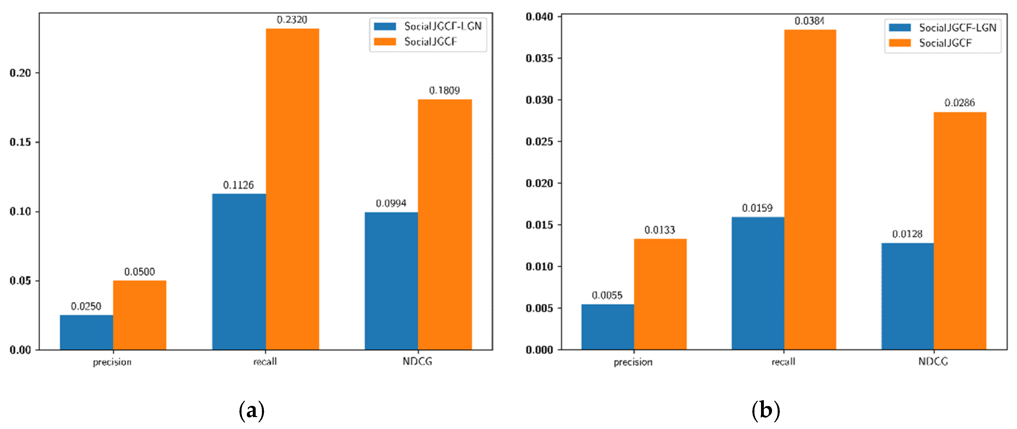
4.3. Comparisons of Graph Fusion Methods

To demonstrate the proposed graph fusion method used in this paper, we compare the performance of SocialJGCF with the graph fusion method used in SocialLGN [40], which is a modification of GraphSage fusion [18]. The fusion method in GraphSage simply adopts concatenation as the fusion method,

$$E_{GraphSage}=\sigma \left(W\left(E_S\left|\right|E_{UI}\right)\right),$$

while SocialLGN applies different weight matrices before concatenation,

$$E_{SocialLGN}=W_3[\sigma (W_2{E}_S)||\sigma (W_1{E}_{UI})].$$

Figure 2 shows the comparison results. The graph fusion method used in this paper achieves approximately 2× recommendation performance for all three metrics and on both datasets.

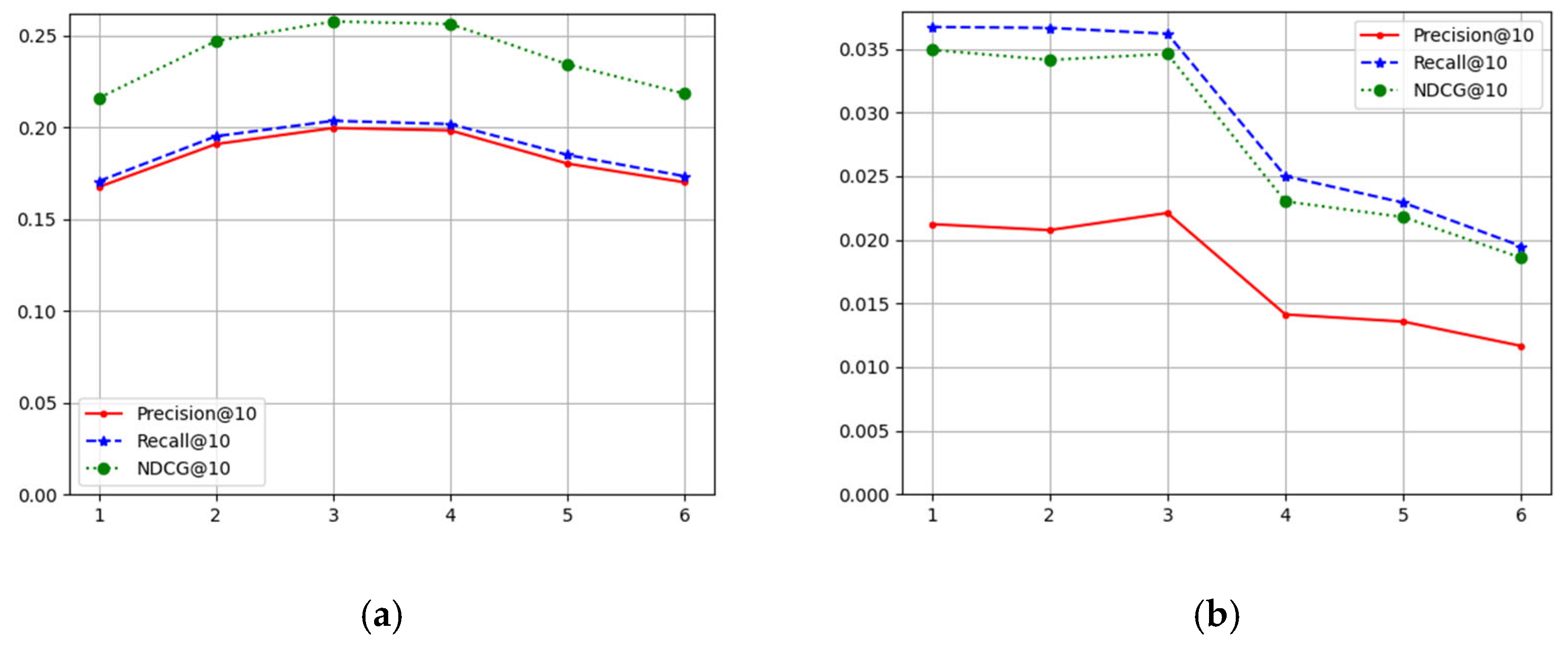
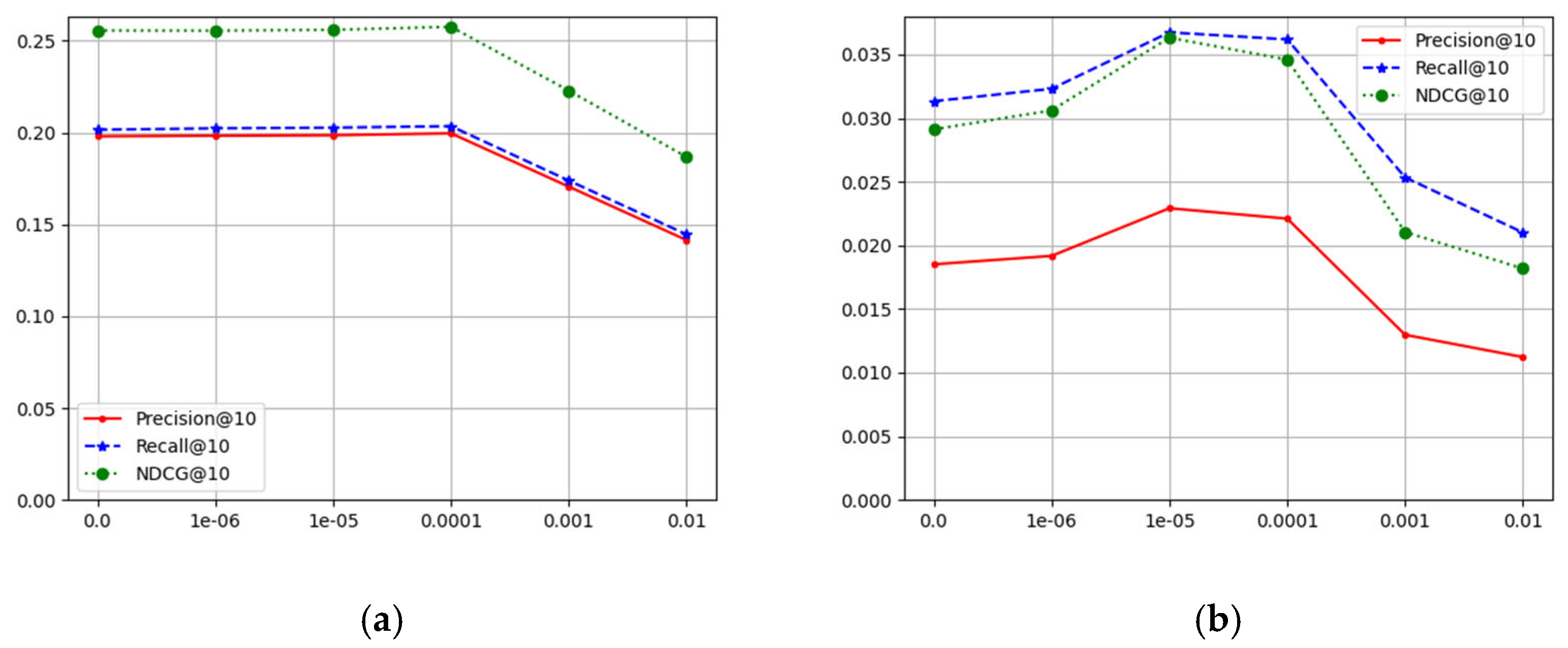
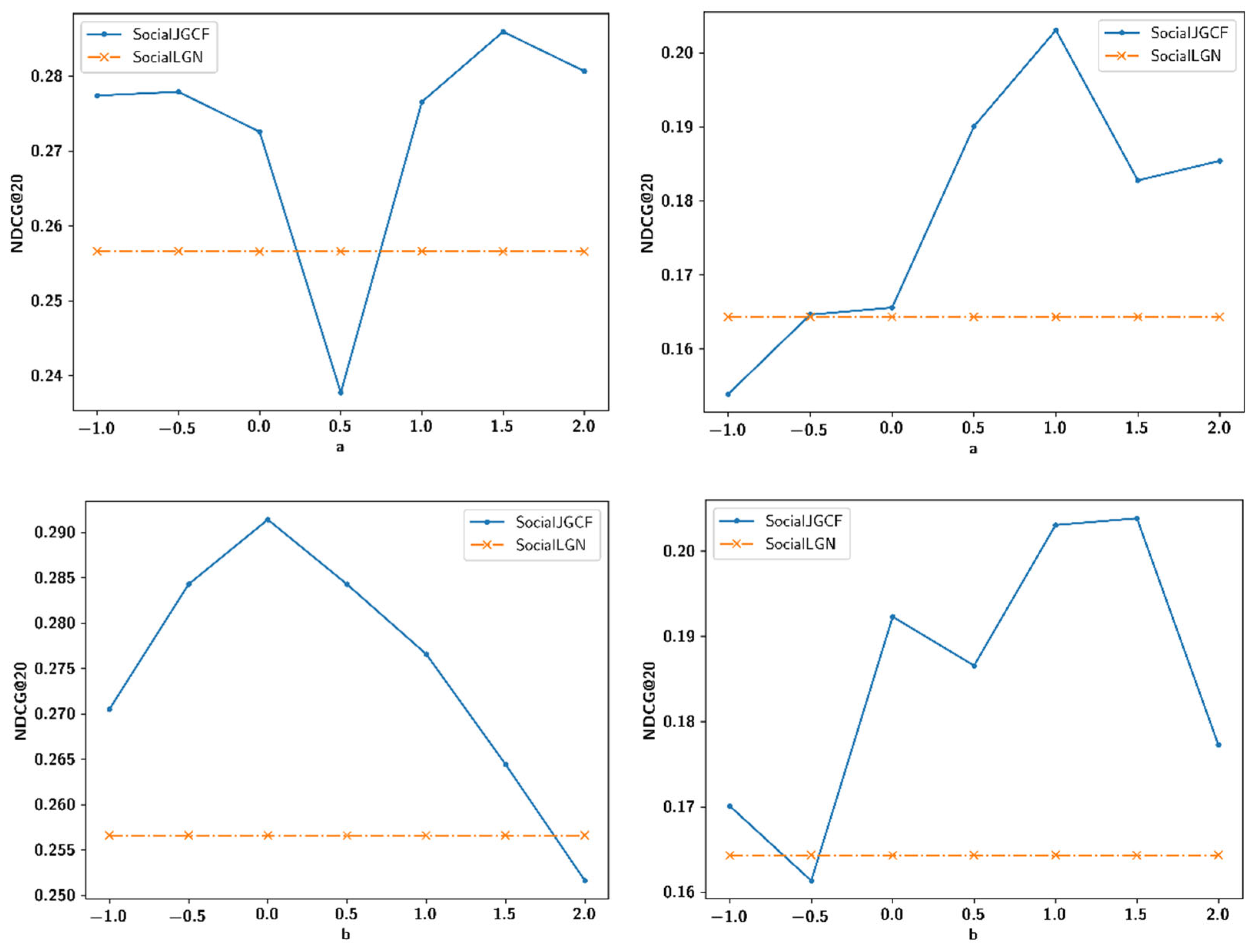
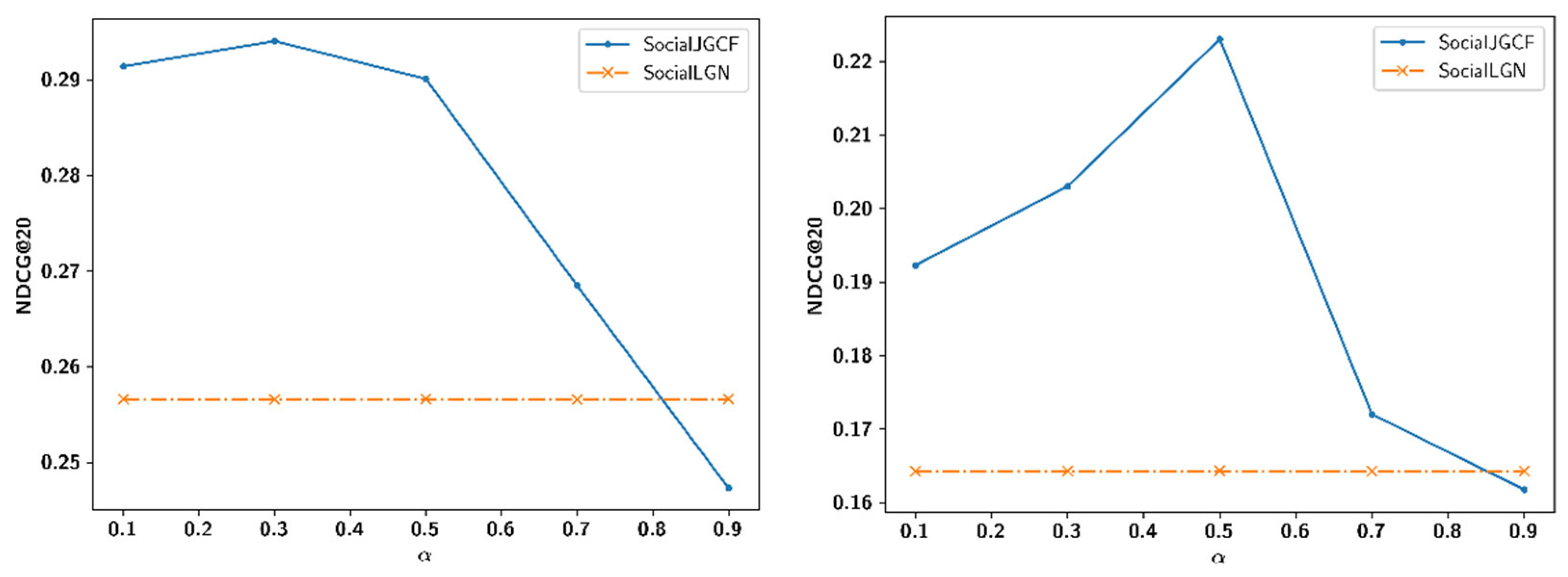
4.4. Sensitivity Analysis for Hyperparameters

In this section, a sensitivity analysis for number of layers $K$ and regularization coefficient $\lambda$ is reported. For analysis of $K$, $K$ varies from 1 to 6 while $\lambda$ = 1 × 10⁻⁴. For analysis of $\lambda$, $K$ is fixed at 3 and $\lambda$ is chosen from {0, 1 × 10⁻⁶, 1 × 10⁻⁵, 1 × 10⁻⁴, 1 × 10⁻³, 1 × 10⁻²}.

Figure 3 shows the sensitivity analysis for $K$. On the LastFM dataset, the performance of SocialJGCF improves rapidly with $K$ before $K=3$ and starts to decrease after $K=4$. On the epinions dataset, the performance of SocialJGCF decreases dramatically when $K\ge 4$. Overall, when $K=3$, SocialJGCF has the best performance on the two datasets.

Figure 4 shows the sensitivity analysis for $\lambda$. On the LastFM dataset, the model achieves the best performance at $\lambda$ = 1 × 10⁻⁴ and a larger regularization coefficient drastically reduces the performance. On the epinions dataset, the model performs best at $\lambda$ = 1 × 10⁻⁵ for the original dataset, but when $\lambda$ = 1 × 10⁻⁴, the model has better performance in the cold-start problem, and any larger regularization coefficient greatly reduces the performance. The result shows that the SocialJGCF is sensitive to regularization and easy to overfit.

Compared with LightGCN, which is adopted by SocialLGN, JGCF comes with additional hyperparameters $a, b$ and $\alpha$, which control the graph filter and band-pass in JGCF. Figure 5 shows the recommendation performance on the LastFM dataset with different $a, b$ and $\alpha$ values. We fix $b=1.0$ and $\alpha =0.1$ when comparing the performance of different $a$ values and fix $a=1.0$ and $\alpha =0.1$ for different $b$ values to make fair comparisons. For the original dataset, $b$ cannot be too large since a large $b$ emphasizes low-frequency signals and thus smooths the dataset.

5. Conclusions

This paper introduces a novel social recommender system based on JGCF. In this model, the user–item interaction graph and social graph propagate independently, and, in the end, user embeddings from the interaction graph and social graph are linearly combined to form the final user embedding, while the final item embedding comes from the propagation of the interaction graph. SocialJGCF is compared with other baseline methods on two real-world datasets, and the results demonstrate that the SocialJGCF has better recommendation performance, especially for the cold-start problem. The time and space complexity analysis demonstrates that SocialJGCF exhibits computationally efficient memory usage and computational performance. The sensitivity analysis of hyperparameters reveals the relationship between model performance and hyperparameter settings, offering guidance for the optimization of SocialJGCF models.

References

1. Koren, Y.; Bell, R.; Volinsky, C. Matrix Factorization Techniques for Recommender Systems. Computer 2009, 42, 30–37. [Google Scholar] [CrossRef]
2. Covington, P.; Adams, J.; Sargin, E. Deep Neural Networks for YouTube Recommendations. In Proceedings of the 10th ACM Conference on Recommender Systems (RecSys ’16), Boston, MA, USA, 15–19 September 2016; Association for Computing Machinery: New York, NY, USA, 2016; pp. 191–198. [Google Scholar]
3. Gao, C.; Wang, X.; He, X.; Li, Y. Graph Neural Networks for Recommender System. In Proceedings of the Fifteenth ACM International Conference on Web Search and Data Mining (WSDM ’22), Tempe, AZ, USA, 21–25 February 2022; Association for Computing Machinery: New York, NY, USA, 2022; pp. 1623–1625. [Google Scholar] [CrossRef]
4. Cialdini, R.B.; Goldstein, N.J. Social influence: Compliance and conformity. Annu. Rev. Psychol. 2004, 55, 591–621. [Google Scholar] [CrossRef] [PubMed]
5. Yu, J.; Yin, H.; Li, J.; Gao, M.; Huang, Z.; Cui, L. Enhance social recommendation with adversarial graph convolutional networks. IEEE Trans. Knowl. Data Eng. 2020, 34, 3727–3739. [Google Scholar] [CrossRef]
6. Ma, H.; Zhou, D.; Liu, C.; Lyu, M.R.; King, I. Recommender systems with social regularization. In Proceedings of the Fourth ACM International Conference on Web Search and Data Mining (WSDM ’11), Hong Kong, China, 9–12 February 2011; Associationfor Computing Machinery: New York, NY, USA, 2011; pp. 287–296. [Google Scholar]
7. Wu, L.; Sun, P.; Fu, Y.; Hong, R.; Wang, X.; Wang, M. A Neural Influence Diffusion Model for Social Recommendation. In Proceedings of the 42nd International ACM SIGIR Conference on Research and Development in Information Retrieval (SIGIR’19), Paris, France, 21–25 July 2019; Association for Computing Machinery: New York, NY, USA, 2019; pp. 235–244. [Google Scholar]
8. Guo, G.; Zhang, J.; Yorke-Smith, N. TrustSVD: Collaborative filtering with both the explicit and implicit influence of user trust and of item ratings. In Proceedings of the AAAI, Austin, TX, USA, 25–30 January 2015; pp. 123–129. [Google Scholar]
9. Wu, S.; Sun, F.; Zhang, W.; Xie, X.; Cui, B. Graph Neural Networks in Recommender Systems: A Survey. ACM Comput. Surv. 2022, 55, 97. [Google Scholar] [CrossRef]
10. Sharma, K.; Lee, Y.C.; Nambi, S.; Salian, A.; Shah, S.; Kim, S.W.; Kumar, S. A survey of graph neural networks for social recommender systems. ACM Comput. Surv. 2024, 56, 265. [Google Scholar] [CrossRef]
11. Fan, W.; Ma, Y.; Li, Q.; He, Y.; Zhao, E.; Tang, J.; Yin, D. Graph Neural Networks for Social Recommendation. In Proceedings of the The World Wide Web Conference (WWW ’19), San Francisco, CA, USA, 13–17 May 2019; Association for Computing Machinery: New York, NY, USA, 2019; pp. 417–426. [Google Scholar]
12. Wu, Q.; Zhang, H.; Gao, X.; He, P.; Weng, P.; Gao, H.; Chen, G. Dual graph attention networks for deep latent representation of multifaceted social effects in recommender systems. In Proceedings of the WWW Conference, San Francisco, CA, USA, 13–17 May 2019; pp. 2091–2102. [Google Scholar]
13. Wu, L.; Li, J.; Sun, P.; Hong, R.; Ge, Y.; Wang, M. Diffnet++: A neural influence and interest diffusion network for social recommendation. IEEE Trans. Knowl. Data Eng. 2020, 34, 4753–4766. [Google Scholar] [CrossRef]
14. Chen, T.; Wong, R.C.-W. An efficient and effective framework for session-based social recommendation. In Proceedings of the WSDM Conference, Virtual, 8–12 March 2021; pp. 400–408. [Google Scholar]
15. Zhou, J.; Cui, G.; Hu, S.; Zhang, Z.; Yang, C.; Liu, Z.; Wang, L.; Li, C.; Sun, M. Graph neural networks: A review of methods and applications. AI Open 2020, 1, 57–81. [Google Scholar] [CrossRef]
16. Wang, S.; Hu, L.; Wang, Y.; He, X.; Sheng, Q.Z.; Orgun, M.A.; Cao, L.; Ricci, F.; Yu, P.S. Graph learning based recommender systems: A review. In Proceedings of the 30th International Joint Conference on Artificial Intelligence, IJCAI 2021, Montreal, QC, Canada, 19–27 August 2021. [Google Scholar]
17. Kipf, T.N.; Welling, M. Semi-supervised classification with graph convolutional networks. In Proceedings of the 5th International Conference on Learning Representations—ICLR 2017 Conference Track, Toulon, France, 24–26 April 2017. [Google Scholar]
18. Hamilton, W.L.; Ying, R.; Leskovec, J. Inductive representation learning on large graphs. In Proceedings of the 31st International Conference on Neural Information Processing Systems, Long Beach, NY, USA, 4–9 December 2017; Curran Associates Inc.: New York, NY, USA, 2017. [Google Scholar]
19. He, X.; Deng, K.; Wang, X.; Li, Y.; Zhang, Y.; Wang, M. LightGCN: Simplifying and Powering Graph Convolution Network for Recommendation. In Proceedings of the 43rd International ACM SIGIR Conference on Research and Development in Information Retrieval (SIGIR ’20), Virtual, 25–30 July 2020; Association for Computing Machinery: New York, NY, USA, 2020; pp. 639–648. [Google Scholar]
20. Wang, X.; He, X.; Wang, M.; Feng, F.; Chua, T.-S. Neural graph collaborative filtering. In Proceedings of the SIGIR Conference, Paris, France, 21–25 July 2019; pp. 165–174. [Google Scholar]
21. Tan, Q.; Liu, N.; Zhao, X.; Yang, H.; Zhou, J.; Hu, X. Learning to hash with graph neural networks for recommender systems. In Proceedings of the WWW Conference, Taiwan, 20–24 April 2020; pp. 1988–1998. [Google Scholar]
22. Mu, N.; Zha, D.; He, Y.; Tang, Z. Graph Attention Networks for Neural Social Recommendation. In Proceedings of the 2019 IEEE 31st International Conference on Tools with Artificial Intelligence (ICTAI), Portland, OR, USA, 4–6 November 2019; pp. 1320–1327. [Google Scholar] [CrossRef]
23. Wang, Z.; Wang, Z.; Li, X.; Yu, Z.; Guo, B.; Chen, L.; Zhou, X. Exploring Multi-Dimension User-Item Interactions with Attentional Knowledge Graph Neural Networks for Recommendation. IEEE Trans. Big Data 2023, 9, 212–226. [Google Scholar] [CrossRef]
24. Wu, B.; Zhong, L.; Yao, L.; Ye, Y. EAGCN: An Efficient Adaptive Graph Convolutional Network for Item Recommendation in Social Internet of Things. IEEE Internet Things J. 2022, 9, 16386–16401. [Google Scholar] [CrossRef]
25. Qian, T.; Liang, Y.; Li, Q.; Xiong, H. Attribute Graph Neural Networks for Strict Cold Start Recommendation. IEEE Trans. Knowl. Data Eng. 2022, 34, 3597–3610. [Google Scholar] [CrossRef]
26. Yu, J.; Yin, H.; Xia, X.; Chen, T.; Cui, L.; Nguyen, Q.V.H. Are Graph Augmentations Necessary? Simple Graph Contrastive Learning for Recommendation. In Proceedings of the 45th International ACM SIGIR Conference on Research and Development in Information Retrieval (SIGIR ’22), Madrid, Spain, 11–15 July 2022; Association for Computing Machinery: New York, NY, USA, 2022; pp. 1294–1303. [Google Scholar]
27. Guo, J.; Du, L.; Chen, X.; Ma, X.; Fu, Q.; Han, S.; Zhang, D.; Zhang, Y. On Manipulating Signals of User-Item Graph: A Jacobi Polynomial-based Graph Collaborative Filtering. In Proceedings of the 29th ACM SIGKDD Conference on Knowledge Discovery and Data Mining (KDD ’23), Long Beach, CA, USA, 6–10 August 2023; Association for Computing Machinery: New York, NY, USA, 2023; pp. 602–613. [Google Scholar]
28. Chen, L.; Wu, L.; Hong, R.; Zhang, K.; Wang, M. Revisiting graph based collaborative filtering: A linear residual graph convolutional network approach. In Proceedings of the AAAI Conference, Vancouver, BC, Canada, 20–27 February 2020; pp. 27–34. [Google Scholar]
29. Li, C.; Jia, K.; Shen, D.; Shi, C.J.; Yang, H. Hierarchical representation learning for bipartite graphs. In Proceedings of the IJCAI Conference, Macao, China, 10–16 August 2019; pp. 2873–2879. [Google Scholar]
30. Ying, R.; He, R.; Chen, K.; Eksombatchai, P.; Hamilton, W.L.; Leskovec, J. Graph Convolutional Neural Networks for Web-Scale Recommender Systems. In Proceedings of the 24th ACM SIGKDD International Conference on Knowledge Discovery & Data Mining (KDD ’18), London, UK, 19–23 August 2018; Association for Computing Machinery: New York, NY, USA, 2018; pp. 974–983. [Google Scholar] [CrossRef]
31. Chang, J.; Gao, C.; He, X.; Jin, D.; Li, Y. Bundle Recommendation with Graph Convolutional Networks. In Proceedings of the 43rd International ACM SIGIR Conference on Research and Development in Information Retrieval (SIGIR ’20), Virtual, 25–30 July 2020; Association for Computing Machinery: New York, NY, USA, 2020; pp. 1673–1676. [Google Scholar] [CrossRef]
32. Ma, H.; King, I.; Lyu, M.R. Learning to recommend with social trust ensemble. In Proceedings of the SIGIR Conference, Boston, MA, USA, 19–23 July 2009; pp. 203–210. [Google Scholar]
33. Li, X.; Sun, L.; Ling, M.; Peng, Y. A survey of graph neural network based recommendation in social networks. Neurocomputing 2023, 549, 126441. [Google Scholar] [CrossRef]
34. Jamali, M.; Ester, M. A matrix factorization technique with trust propagation for recommendation in social networks. In Proceedings of the Fourth ACM Conference on Recommender Systems (RecSys ’10), Barcelona, Spain, 26–30 September 2010; Association for Computing Machinery: New York, NY, USA, 2010; pp. 135–142. [Google Scholar]
35. Mandal, S.; Maiti, A. Graph Neural Networks for Heterogeneous Trust based Social Recommendation. In Proceedings of the 2021 International Joint Conference on Neural Networks (IJCNN), Shenzhen, China, 18–22 July 2021; pp. 1–8. [Google Scholar] [CrossRef]
36. Lin, W.; Gao, Z.; Li, B. Guardian: Evaluating Trust in Online Social Networks with Graph Convolutional Networks. In Proceedings of the IEEE INFOCOM 2020—IEEE Conference on Computer Communications, Toronto, ON, Canada, 6–9 July 2020; pp. 914–923. [Google Scholar] [CrossRef]
37. Salamat, A.; Luo, X.; Jafari, A. HeteroGraphRec: A heterogeneous graph-based neural networks for social recommendations. Knowl.-Based Syst. 2021, 217, 106817. [Google Scholar] [CrossRef]
38. Song, W.; Xiao, Z.; Wang, Y.; Charlin, L.; Zhang, M.; Tang, J. Session-Based Social Recommendation via Dynamic Graph Attention Networks. In Proceedings of the Twelfth ACM International Conference on Web Search and Data Mining (WSDM ’19), Melbourne, Australia, 11–15 February 2019; Association for Computing Machinery: New York, NY, USA, 2019; pp. 555–563. [Google Scholar] [CrossRef]
39. Han, H.; Zhang, M.; Hou, M.; Zhang, F.; Wang, Z.; Chen, E.; Wang, H.; Ma, J.; Liu, Q. STGCN: A spatial-temporal aware graph learning method for POI recommendation. In Proceedings of the 2020 IEEE International Conference on Data Mining (ICDM), Sorrento, Italy, 17–20 November 2020; pp. 1052–1057. [Google Scholar]
40. Liao, J.; Zhou, W.; Luo, F.; Wen, J.; Gao, M.; Li, X.; Zeng, J. SocialLGN: Light graph convolution network for social recommendation. Inf. Sci. 2022, 589, 595–607. [Google Scholar] [CrossRef]
41. Guo, Z.; Wang, H. A Deep Graph Neural Network-Based Mechanism for Social Recommendations. IEEE Trans. Ind. Inform. 2021, 17, 2776–2783. [Google Scholar] [CrossRef]
42. Xu, H.; Huang, C.; Xu, Y.; Xia, L.; Xing, H.; Yin, D. Global Context Enhanced Social Recommendation with Hierarchical Graph Neural Networks. In Proceedings of the 2020 IEEE International Conference on Data Mining (ICDM), Sorrento, Italy, 17–20 November 2020; pp. 701–710. [Google Scholar]
43. Rendle, S.; Freudenthaler, C.; Gantner, Z.; Schmidt-Thieme, L. BPR: Bayesian personalized ranking from implicit feedback. In Proceedings of the Twenty-Fifth Conference on Uncertainty in Artificial Intelligence (UAI ’09), Montreal, Canada, 18–21 June 2009; AUAI Press: Arlington, VA, USA, 2019; pp. 452–461. [Google Scholar]
Figure 1. (a) Overall architecture of SocialJGCF. (b) Detailed structure of JGCF.
Applsci 14 12070 g001
Figure 2. Comparison of different graph fusion methods. (a) LastFM. (b) epinions.
Applsci 14 12070 g002
Figure 3. Sensitivity analysis for K . (a) LastFM. (b) epinions.
Applsci 14 12070 g003
Figure 4. Sensitivity analysis for λ . (a) LastFM. (b) epinions.
Applsci 14 12070 g004
Figure 5. Analysis for a ,     b and α . Results for the original LastFM dataset and cold-start LastFM dataset are shown in the left and right columns.
Applsci 14 12070 g005aApplsci 14 12070 g005b