Transformer–BiLSTM Fusion Neural Network for Short-Term PV Output Prediction Based on NRBO Algorithm and VMD

Abstract

In order to solve the difficulties that the uncertain characteristics of PV output, such as volatility and intermittency, will bring to the development of microgrid scheduling plans, this paper proposes a Transformer–Bidirectional Long Short-Term Memory (BiLSTM) neural network PV power generation forecasting fusion model based on the Newton–Raphson optimization algorithm (NRBO) and Variational Modal Decomposition (VMD). Firstly, the principle of the VMD technique and the Gray Wolf Optimization (GWO) algorithm’s key parameter optimization method for VMD are introduced. Then, the Transformer decoder partially fuses the BiLSTM network and retains the encoder to obtain the body of the prediction model, followed by explaining the principle of the NRBO algorithm. And finally, the VMD-NRBO-Transformer-BiLSTM prediction model and hyperparameter selection are evaluated by the NRBO algorithm. The algorithm sets up a multi-model comparison experiment, and the results show that the prediction model proposed in this paper has the best prediction accuracy and the optimal evaluation index.

1. Introduction

With the increasing global energy demand and the depletion of fossil fuel reserves, the growing contradiction between the limited availability of fossil energy resources and the rising energy demand has become increasingly evident. Reducing reliance on non-renewable energy sources is essential for ensuring the sustainable development of society [1]. However, the generation of renewable energy, particularly photovoltaic (PV) power, is significantly influenced by climate and environmental factors, leading to inherent uncertainty and volatility in PV power output. This, in turn, presents challenges for the stable operation of power systems [2]. In response to these challenges, advancements in statistical methods and artificial intelligence (AI) technologies have facilitated the continuous development of various photovoltaic power forecasting approaches, which can be categorized into three timescales: medium- to long-term, short-term, and very short-term forecasts [3]. However, traditional statistical methods primarily rely on historical data and often fail to account for the impact of weather conditions. In contrast, AI-based techniques can directly predict PV power output by training on large datasets that incorporate both historical data and atmospheric variables, offering a more robust solution that does not require the extensive input data typical of statistical methods.

In recent years, the rapid advancement of deep learning technologies has provided new opportunities for photovoltaic power forecasting. Common models include BackPropagation (BP) neural networks, support vector machines (SVMs), radial basis function (RBF) neural networks, and Long Short-Term Memory (LSTM) networks, all of which have been widely used in PV power forecasting and have yielded promising results [4]. For instance, the paper [5] proposed a short-term power forecasting method for new energy generation by selecting a wide range of meteorological features and optimizing the parameters of the SVM model. They employed Particle Swarm Optimization (PSO) to enhance the model’s prediction accuracy for renewable energy generation. However, such methods often fail to adequately model the complex nonlinear temporal features and long-term dependencies inherent in wind and solar power generation. The authors of [6] conducted a short-term PV power forecasting study using a BP neural network optimized by Ant Colony Optimization (ACO). They incorporated gray relational analysis to identify key factors influencing PV generation, improving the model’s prediction accuracy. Despite this, BP neural networks are prone to issues such as vanishing gradients and local optima, and they struggle to effectively model time-series data. These methods also do not fully exploit the potential of deep learning architectures, such as Recurrent Neural Networks (RNNs) or LSTMs, which are better suited for handling sequential data. The study [7] applied a bidirectional LSTM network to forecast PV power generation under various weather conditions, demonstrating that this approach outperformed traditional machine learning algorithms in terms of both accuracy and stability. However, their model did not fully address the generalization ability across different regions or for long-term forecasts, and it lacked an evaluation of robustness under extreme weather events or sudden changes. López Santos et al. used the Temporal Fusion Transformer (TFT) model for next-day PV power forecasting, combining attention mechanisms with multi-timescale temporal dynamics. Their results showed that the TFT model outperformed traditional algorithms in prediction accuracy across multiple facilities [8]. However, the model’s high complexity and its substantial requirements for data, computation, and storage resources could present challenges in resource-constrained environments.

Combining multiple network models to form a combinatorial neural network is gradually becoming a mainstream method to improve prediction accuracy. The literature [9] proposed an intelligent multi-model prediction method based on output characteristic clustering and Convolutional Neural Network–Long Short-Term Memory (CNN-LSTM) for photovoltaic (PV) power generation interval prediction. The combination of the CNN and LSTM effectively improves the modeling accuracy of the intelligent prediction model. The literature [10] proposed an LSTM-Informer model based on the Improved Stacked Ensemble Algorithm (ISt-LSTM-Informer). By integrating the advantages of the two underlying models, the ISt-LSTM-Informer achieves accurate short- and medium-term PV power prediction. The literature [11] proposed an integrated multivariate model based on VMD, a CNN, and a bidirectional gated recurrent unit (BiGRU), which effectively improves the accuracy of prediction. However, none of the above literature considered the optimization of the hyperparameters of neural networks, and the settings of the hyperparameters were selected based on experience, which could not be adaptively adjusted according to the actual scene.

In order to realize accurate PV power generation prediction, this paper proposes a combined network prediction model, which integrates NRBO, VMD, and Transformer–BiLSTM. The Transformer decoder partially fuses the BiLSTM network and retains the encoder to obtain the main body of the prediction model, and at the same time, the NRBO algorithm is applied to optimize the relevant hyperparameters of the network model. The NRBO algorithm is used to optimize the hyperparameters of the network model. The VMD of historical PV data is performed to remove the noise and redundant signals, and the GWO algorithm is applied to optimize the key parameters of the VMD. The characteristic parameters related to PV output are selected as inputs to the model, and the predicted values of each modal component are superimposed to obtain the final PV output power.

2. Principle of VMD

Variational Mode Decomposition (VMD) is a data processing technique introduced by Dragomiretskiy et al. [12] in 2014. It is particularly effective in handling dynamic, non-stationary, and nonlinear complex signals. By decomposing the original signal under specific constraints, VMD facilitates signal denoising, enhancing the quality of the data for subsequent analysis.

2.1. Construction of the Variational Constrained Model

The number of Intrinsic Mode Function (IMF) components, denoted as K, is pre-determined, with the objective of minimizing the bandwidth. The finite bandwidth and central frequency of each IMF are iteratively optimized to achieve the optimal decomposition of the signal [13,14,15]. The model is expressed as follows:

$$\left\{\begin{array}{l}\underset{\left\{u_k\right\},\left\{{\omega }_k\right\}}{\min }\left\{{\displaystyle \sum _{k=1}^K{‖{\mathit{\partial }}_{\mathit{t}}\left[\left(\delta (\mathit{t})+\frac{\mathrm{j}}{\mathsf{\pi }\mathit{t}}\right)\otimes u_k(\mathit{t})\right]e^{-\mathrm{j}{\omega }_k\mathit{t}}‖}_2^2}\right\}\\ \mathrm{s}.\mathrm{t}.{\displaystyle \sum _{k=1}^K{u}_k}(\mathit{t})=f(\mathit{t})\end{array}\right.$$

(1)

Here, $u_k$ represents the k-th IMF component. ${\omega }_k$ represents the corresponding central frequency of the IMF component. $\delta (\mathit{t})$ is the Dirac delta function. ${\mathit{\partial }}_{\mathit{t}}$ represents the partial derivative with respect to time t. $\otimes$ represents the convolution operator. Additionally, $f(\mathit{t})$ represents the original signal and j represents the imaginary unit.

2.2. Constrained Model Solving

To overcome the aforementioned constraints, the constrained variational problem is decoupled by introducing a Lagrange multiplier $\lambda (\mathit{t})$ and second-order penalty factor α, leading to the formulation of a new augmented Lagrangian Optimization Model [16], which is expressed as follows:

$$\begin{array}{l}L\left(\left\{u_k\right\},\left\{{\omega }_k\right\},\lambda \right)=\alpha {\displaystyle \sum _{k=1}^K{‖\left[{\mathit{\partial }}_{\mathit{t}}\left(\delta (\mathit{t})+\frac{\mathrm{j}}{\mathsf{\pi }\mathit{t}}\right)\otimes u_k(\mathit{t})\right]{\mathrm{e}}^{-\mathrm{j}{\omega }_k\mathit{t}}‖}_2^2}\\ +{‖f(\mathit{t})-{\displaystyle \sum _{k=1}^K{u}_k(\mathit{t})}‖}_2^2+〈\lambda (\mathit{t}),f(\mathit{t})-{\displaystyle \sum _{k=1}^K{u}_k(\mathit{t})}〉\end{array}$$

(2)

The Alternating Direction Method of Multipliers (ADMM) is employed to solve the unconstrained problem. By integrating Fourier equidistant transformation, alternating optimization is applied to λ, $u_k$, and ${\omega }_k$, as expressed below:

$${\widehat{u}}_k^{n+1}(\omega )={\displaystyle \frac{f(\omega )-{\displaystyle \sum _{i<k}{\widehat{u}}_i^{n+1}}(\omega )+\frac{{\widehat{\lambda }}^n\left(\omega \right)}{2}}{1+2\alpha {\left(\omega -{\omega }_k^n\right)}^2}}$$

(3)

$${\omega }_k^{n+1}={\displaystyle \frac{{\displaystyle {\int }_0^{\infty }\omega }{\left|{\widehat{u}}_k^{n+1}(\omega )\right|}^2\mathrm{d}\omega }{{\displaystyle {\int }_0^{\infty }{\left|{\widehat{u}}_k^{n+1}(\omega )\right|}^2}\mathrm{d}\omega }}$$

(4)

$${\widehat{\lambda }}^{n+1}(\omega )={\widehat{\lambda }}^n(\omega )+\tau \left(f(\omega )-{\displaystyle \sum _{i<k}{\widehat{p}}_i^{n+1}}(\omega )\right)$$

(5)

Here, τ represents the noise tolerance. ${\widehat{u}}_k^{n+1}(\omega )$ and ${\widehat{\lambda }}^{n+1}(\omega )$ are the Fourier transforms of $u_k(\mathit{t})$ and $\lambda (\mathit{t})$, respectively.

In VMD, the modulus number K and the penalty factor $\alpha$ are two important factors affecting the decomposition results, the determination of the K value determines the effective degree of information extraction, and $\alpha$ affects the bandwidth of the IMF component, which determines whether there is signal loss and signal confusion. Therefore, the selection of VMD parameters is of great significance to the data decomposition, and the manual selection of parameters often does not obtain the best signal decomposition results, so this paper adopts the GWO algorithm [17] to optimize the parameters.

GWO is inspired by the hunting and predatory activities of gray wolves, and its principle is to divide the wolf pack into four classes, A₁, A₂, A₃, and A₄, and to realize the renewal and iteration of the wolf pack by simulating the wolf pack’s foraging and implementing the three behaviors of encircling, hunting, and attacking. The optimization process is shown in Figure 1, where H is the maximum number of iterations and h is the current number of iterations.

3. Transformer Encoder-Based BiLSTM Network Model

This paper proposes a network model embedded with BiLSTM, based on the Transformer encoder–decoder architecture. In the encoding phase, the Transformer encoder is utilized to extract features from the input data, while the decoding phase is enhanced by incorporating BiLSTM layers and fully connected layers. This results in the development of a novel Transformer-encoder–BiLSTM-decoder network model.

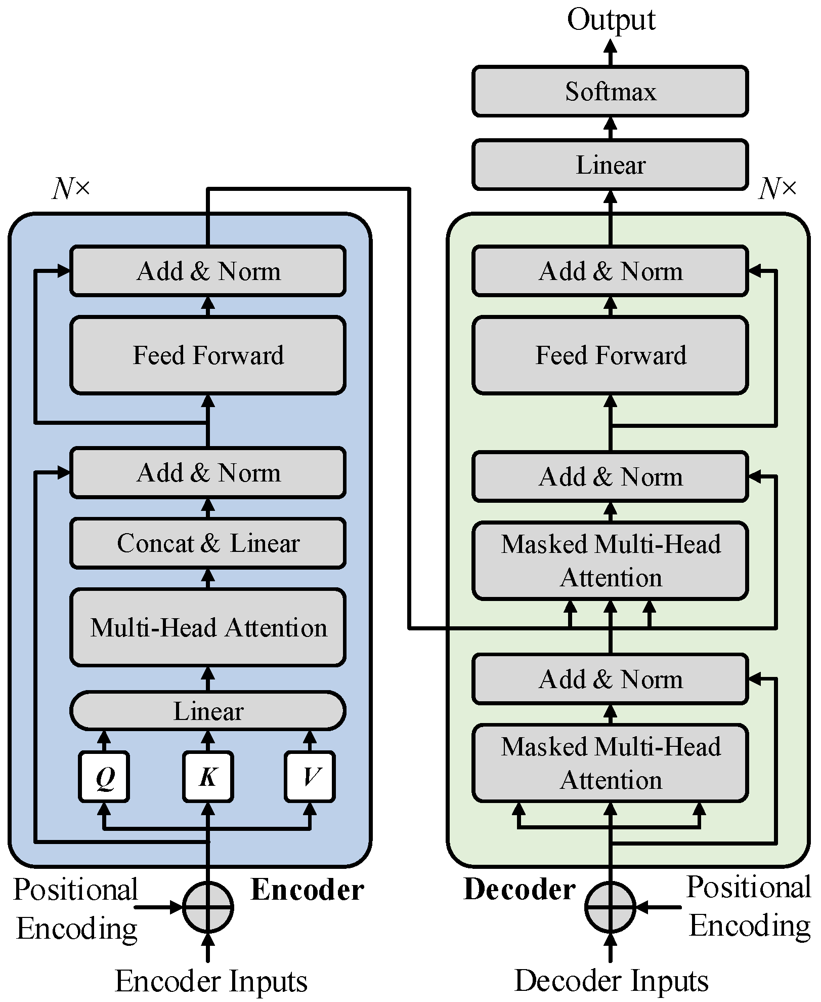
3.1. Feature Extraction of the Transformer Encoder

The structure of the Transformer model is illustrated in Figure 2, consisting of an encoder and a decoder [18,19]. The encoder comprises N = 6 identical layers, each containing a multi-head attention mechanism and a position-wise feedforward neural network sublayer. Residual connections and layer normalization are applied to the output of each sublayer, facilitating the capture of dependencies across all positions in the input sequence. The decoder is similarly composed of N = 6 identical layers, with each layer consisting of three sublayers: a masked self-attention layer, an encoder–decoder attention layer, and a position-wise feedforward neural network. Residual connections and layer normalization are also applied after each sublayer. This architecture ensures that the decoder incorporates information from previous outputs while preventing the influence of future data during sequence generation.

The structure of the Transformer encoder employed in this paper is outlined as follows:

1

Positional Encoding

Traditional Recurrent Neural Networks (RNNs) can inherently capture positional information within sequences. However, the Transformer model lacks built-in mechanisms for encoding sequence positions. To address this limitation, positional encodings are introduced to inject positional information into each element of the input sequence. This enables the model to differentiate between various positions within the input data and ensures the retention of the complete feature set of the input information.

$$\left\{\begin{array}{l}P{E}_{(pos,2i)}=\sin ({\displaystyle \frac{pos}{{10000}^{\frac{2i}{d_{\mathrm{model}}}}}})\\ P{E}_{(pos,2i+1)}=\cos ({\displaystyle \frac{pos}{{10000}^{\frac{2i}{d_{\mathrm{model}}}}}})\end{array}\right.$$

(6)

Here, pos represents the position in the sequence. i represents the dimension. d_model represents the embedding space dimension.

2

Self-Attention

The self-attention mechanism assesses the importance of each position in relation to others by calculating the attention scores between the Query, Key, and Value. It then performs a weighted aggregation of the various components of the input sequence based on these scores [20].

$$A\mathit{t}\mathit{t}en\mathit{t}ion(\mathit{Q},\mathit{K},\mathit{V})=sof\mathit{t}\max ({\displaystyle \frac{\mathit{Q}{\mathit{K}}^{\mathit{T}}}{\sqrt{d_K}}})*\mathit{V}$$

(7)

Here, Q, K, and V represent the Query, Key, and Value matrices, respectively. d_K denotes the dimension of the Key. The sequence information, after positional encoding, is divided into Q, K, and V, which are used as the input to the encoder.

To capture richer sequence features, the Transformer model utilizes multiple self-attention mechanisms operating in parallel. Each attention head learns a distinct set of weights, enabling the model to extract information from different subspaces of the input. The outputs of the h attention heads are concatenated, as shown in the Equation (8). However, since this concatenated result does not provide an integrated representation, a linear transformation is applied to fuse the outputs effectively.

$$\mathrm{MultiHead}(\mathit{Q},\mathit{K},\mathit{V})=\mathrm{Concat}({\mathrm{head}}_1,{\mathrm{head}}_2,...,{\mathrm{head}}_{\mathit{h}}){\mathit{W}}^O$$

(8)

$${\mathrm{head}}_i=A\mathit{t}\mathit{t}en\mathit{t}ion(Q_i,K_i,V_i)$$

(9)

$$Q_i,K_i,V_i=\mathit{Q}{\mathit{W}}_i^Q,\mathit{K}{\mathit{W}}_i^K,\mathit{V}{\mathit{W}}_i^V$$

(10)

Here, head_i represents the output of attention head_i. Q_i, K_i, and V_i are the inputs to attention head_i. ${\mathit{W}}_i^Q$, ${\mathit{W}}_i^K$, ${\mathit{W}}_i^V$, and W^O are the parameter matrices for the linear transformation, where W^O is used for the linear transformation of the concatenated output from multiple attention heads.

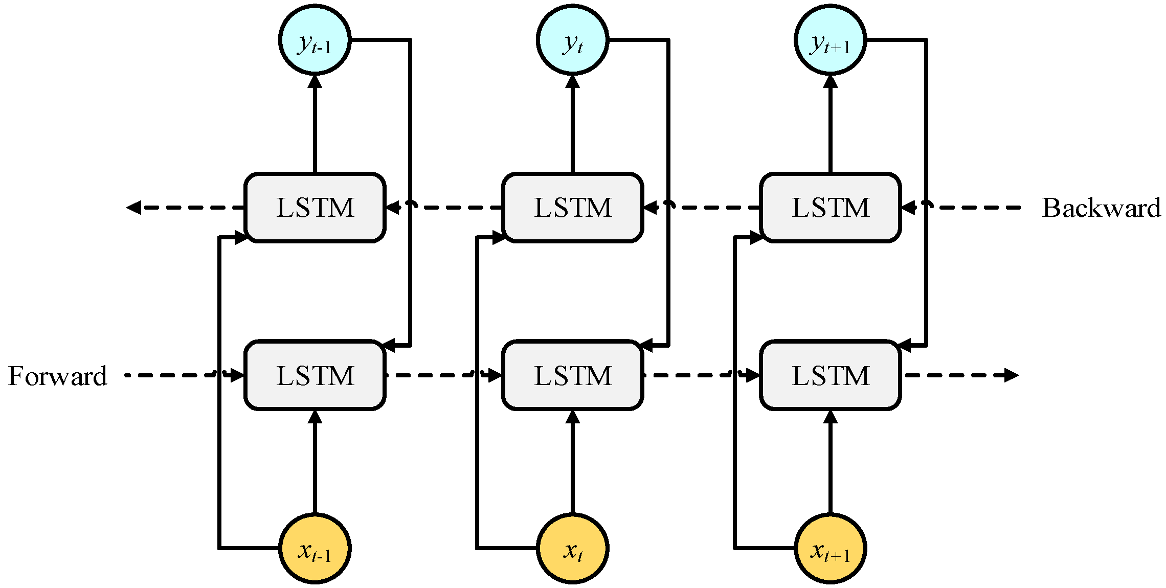
3.2. BiLSTM Network

Long Short-Term Memory (LSTM) networks, a specialized type of Recurrent Neural Network (RNN), are widely used for processing time-series data due to their ability to better capture correlations in sequential information. By incorporating input, forget, and output gate mechanisms, LSTMs regulate the flow of feature information, effectively addressing challenges such as gradient explosion and vanishing gradients that are common in traditional RNNs. The bidirectional LSTM (BiLSTM) network consists of two LSTM components: a forward LSTM that processes the input data in the forward direction, and a backward LSTM that processes the data in the reverse direction, thereby enhancing the network’s ability to capture contextual information from both directions [20,21,22].

The BiLSTM network captures both past and future information simultaneously, effectively modeling bidirectional dependencies in the input data, as illustrated in Figure 3. The input is processed by both the forward and backward BiLSTM components, and their outputs at each time step are concatenated to produce the final output $y_{\mathit{t}}$.

$${\overrightarrow{\mathit{h}}}_{\mathit{t}}=f\left({\overrightarrow{\mathit{W}}}_x{x}_{\mathit{t}}+{\overrightarrow{\mathit{W}}}_{\mathit{h}}{\overrightarrow{\mathit{h}}}_{\mathit{t}-1}+{\overrightarrow{\mathit{b}}}_{\mathit{h}}\right)$$

(11)

$${\overleftarrow{\mathit{h}}}_{\mathit{t}}=\mathit{f}\left({\overleftarrow{\mathit{W}}}_{\mathit{x}}{\mathit{x}}_{\mathit{t}}+{\overleftarrow{\mathit{W}}}_{\mathit{h}}{\overleftarrow{\mathit{h}}}_{\mathit{t}+1}+{\overleftarrow{\mathit{b}}}_{\mathit{h}}\right)$$

(12)

$${\mathit{y}}_{\mathit{t}}=\left[{\overrightarrow{\mathit{h}}}_{\mathit{t}},{\overleftarrow{\mathit{h}}}_{\mathit{t}}\right]$$

(13)

Here, ${\overrightarrow{\mathit{h}}}_{\mathit{t}}$ and ${\overrightarrow{\mathit{h}}}_{\mathit{t}-1}$ represent the LSTM cell state vectors at the corresponding time steps for the forward propagation layer, respectively. ${\overleftarrow{\mathit{h}}}_{\mathit{t}}$ and ${\overleftarrow{\mathit{h}}}_{\mathit{t}+1}$ are the input weight matrices for the forward and backward propagation layers, respectively. ${\overrightarrow{\mathit{W}}}_x$ and ${\overleftarrow{\mathit{W}}}_x$ are the input weight matrices for the forward and backward propagation layers, respectively. ${\overrightarrow{\mathit{W}}}_{\mathit{h}}$ and ${\overleftarrow{\mathit{W}}}_{\mathit{h}}$ are the forget weight matrices for the forward and backward propagation layers, respectively. Finally, ${\overrightarrow{\mathit{b}}}_{\mathit{h}}$ and ${\overleftarrow{\mathit{b}}}_{\mathit{h}}$ are the biases for the forward and backward propagation layers, respectively.

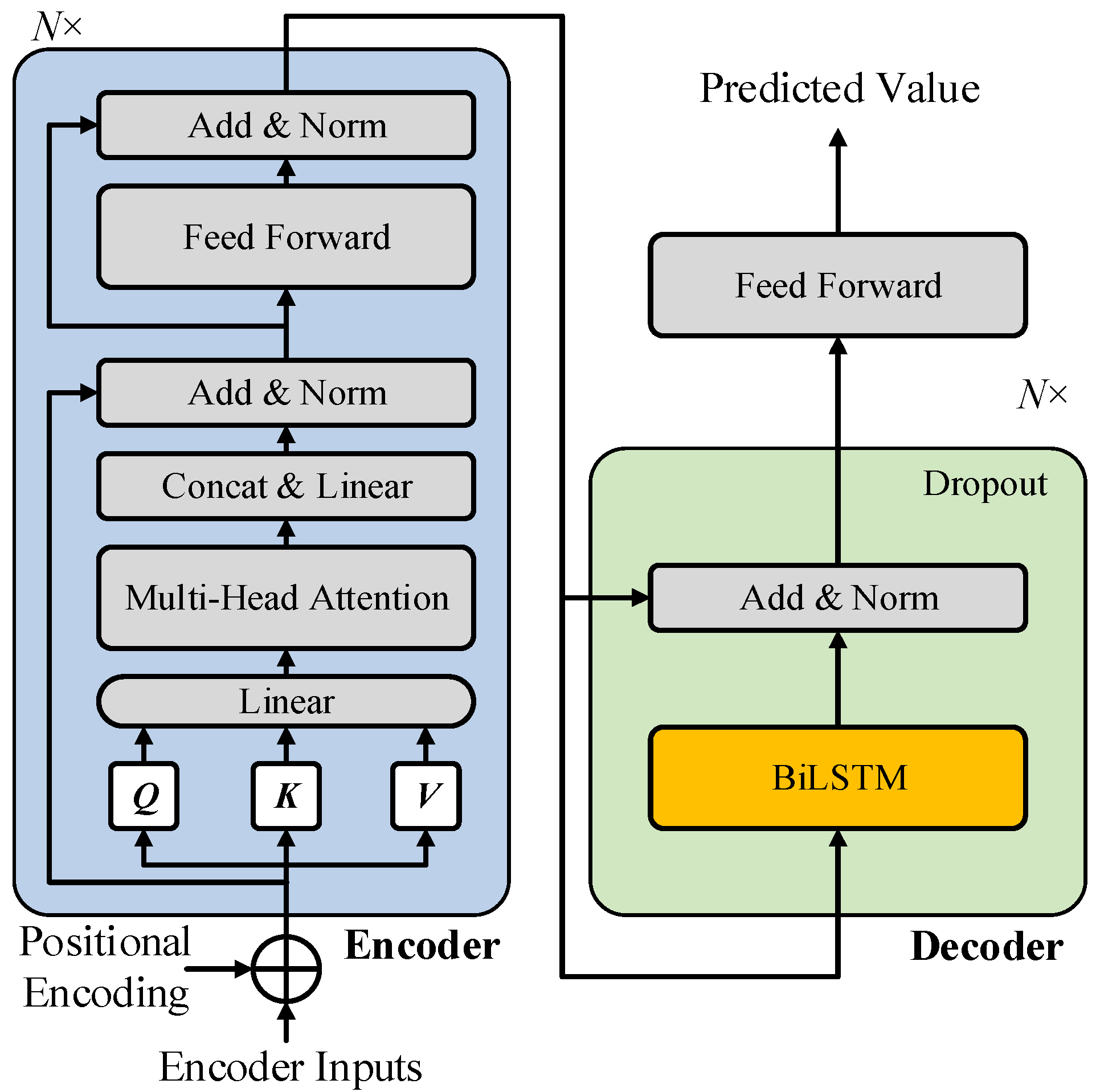
3.3. The Architecture of the Transformer–BiLSTM Model

The traditional Transformer model, when applied to machine translation, employs a masked multi-head attention mechanism, enabling the model to attend to previous text content during sequence generation. This ensures the coherence and logical consistency of the generated text. However, in the context of time-series data prediction, the relationships between data points in a sliding window differ significantly from those in machine translation tasks [22,23]. In time-series forecasting, the model input consists of known historical data, intending to predict future values. To address this, BiLSTM is employed to replace the attention layer in the original Transformer decoder, with residual connections applied to process the input sequence data. This modification preserves the information from the encoder while addressing the long-term dependency problem inherent in sequential data. To mitigate overfitting during model training, a Dropout layer is incorporated within the BiLSTM layer, randomly dropping the outputs of certain neurons. Finally, a fully connected feedforward neural network is used to generate the final prediction. The architecture of the fused Transformer–BiLSTM model is depicted in Figure 4.

$$\left\{\begin{array}{l}{\mathrm{Output}}_1=\mathrm{Dropout}\left(\mathrm{LSTM}\left(x\right)\right)+x\\ {\mathrm{Output}}_N=\mathrm{Dropout}\left(\mathrm{LSTM}\left({\mathrm{Output}}_{N-1}\right)\right)+{\mathrm{Output}}_{N-1}\end{array}\right.$$

(14)

Here, x represents the output of the Transformer encoder.

4. NRBO Algorithm

NRBO defines the search path by utilizing the Newton–Raphson Search Rule (NRSR) in conjunction with the Trap Avoidance Operator (TAO) to effectively explore the search space.

4.1. Population Initialization

NRBO seeks the optimal solution by generating an initial random population within the boundaries of candidate solutions. This process is based on M populations, each containing N decision variables. The initial random population is generated as follows [24].

$$x_n^m=lb+rand\cdot \left(ub-lb\right) m\in [0,M],n\in [1,N]$$

(15)

Here, $x_n^m$ represents the position of the n-th dimension in the m-th population; rand is a random number between 0 and 1; and lb and ub are the lower and upper boundaries, respectively. The generated population matrix is shown below.

$$\mathit{X}=\left[\begin{array}{cccc}{x}_1^1& x_2^1& \cdots & x_{dim}^1\\ x_1^2& x_2^2& \cdots & x_{dim}^2\\ ⋮& ⋮& \ddots & ⋮\\ x_1^{Np}& x_2^{Np}& \cdots & x_{dim}^{Np}\end{array}\right]$$

(16)

4.2. Newton–Raphson Search Rule (NRSR)

The Newton–Raphson Method (NRM) employs Taylor series expansion to iteratively update the solution position, progressively refining it to identify the optimal solution. This approach enhances the exploration capability and accelerates convergence. Starting from a randomly selected initial solution, the subsequent solution position is updated along a specified direction. The position update process is as follows:

$$x^{i\mathit{t}+1}=x^{i\mathit{t}}-{\displaystyle \frac{f^{\prime }\left(x^{i\mathit{t}}\right)}{f^{″}\left(x^{i\mathit{t}}\right)}}$$

(17)

Here, $x^{i\mathit{t}}$ represents the current position of the solution. $x^{i\mathit{t}+1}$ represents the updated position of the solution and $f\left(x\right)$ represents the fitness function.

Based on the Taylor series expansion, the parameter ρ is introduced to guide the population in the correct evolutionary direction, thereby enhancing the efficiency of NRBO. Furthermore, improvements are incorporated based on the NRM proposed in [25,26].

$$\rho =a\cdot \left({\mathit{X}}_{\mathrm{bet}}-{\mathit{X}}_n^{i\mathit{t}}\right)+b\cdot \left({\mathit{X}}_{r_1}^{i\mathit{t}}-{\mathit{X}}_{r_2}^{i\mathit{t}}\right)$$

(18)

$$\mathrm{\Delta }\mathit{X}=rand(1,dim)\cdot \left|{\mathit{X}}_{\mathrm{bet}}-{\mathit{X}}^{i\mathit{t}}\right|$$

(19)

$$\mathrm{NRSR}=randn\cdot {\displaystyle \frac{(Y_{\mathrm{wor}}-Y_{\mathrm{bet}})\cdot \mathrm{\Delta }\mathit{X}}{2(Y_{\mathrm{wor}}+Y_{\mathrm{bet}}-2{\mathit{X}}^{i\mathit{t}})}}$$

(20)

$$Y_{\mathrm{wor}}=r_3\cdot (\mathrm{Mean}(Z^{i\mathit{t}+1}+{\mathit{X}}^{i\mathit{t}})+r_3\mathrm{\Delta }\mathit{X})$$

(21)

$$Y_{\mathrm{bet}}=r_3\cdot (\mathrm{Mean}(Z^{i\mathit{t}+1}+{\mathit{X}}^{i\mathit{t}})-r_3\mathrm{\Delta }\mathit{X})$$

(22)

$${\mathit{Z}}^{i\mathit{t}+1}={\mathit{X}}^{i\mathit{t}}-randn\cdot {\displaystyle \frac{({\mathit{X}}_{\mathrm{wor}}-{\mathit{X}}_{\mathrm{bet}})\cdot \mathrm{\Delta }\mathit{X}}{2({\mathit{X}}_{\mathrm{wor}}+{\mathit{X}}_{\mathrm{bet}}-2{\mathit{X}}^{i\mathit{t}})}}$$

(23)

Here, a and b are random numbers between 0 and 1. ${\mathit{X}}_n^{i\mathit{t}}$ represents the population n after the i-th iteration. NRSR is the NRM-based position update law. randn is a standard normally distributed random number. X_bet and X_wor represent the better and worse populations in the vicinity, respectively. r₁ and r₂ are random integers between 0 and M. Y_wor and Y_bet are two positions generated using $Z^{i\mathit{t}+1}$ and ${\mathit{X}}^{i\mathit{t}}$. r₃ is a random number between 0 and 1. Thus, Equation (17) is updated as follows:

$$\mathit{X}{1}_n^{i\mathit{t}}={\mathit{X}}_n^{i\mathit{t}}-randn\cdot {\displaystyle \frac{(Y_{\mathrm{wor}}-Y_{\mathrm{bet}})\cdot \mathrm{\Delta }{\mathit{X}}_n}{2(Y_{\mathrm{wor}}+Y_{\mathrm{bet}}-2{\mathit{X}}_n^{i\mathit{t}})}}+\rho$$

(24)

By replacing ${\mathit{X}}_n^{i\mathit{t}}$ with the better position X_bet, the new position update formula is obtained:

$$\mathit{X}{2}_n^{i\mathit{t}}={\mathit{X}}_{\mathrm{bet}}-randn\cdot {\displaystyle \frac{(Y_{\mathrm{wor}}-Y_{\mathrm{bet}})\cdot \mathrm{\Delta }{\mathit{X}}_n}{2(Y_{\mathrm{wor}}+Y_{\mathrm{bet}}-2{\mathit{X}}_n^{i\mathit{t}})}}+\rho$$

(25)

The Equation (24) is effective for local search but has limitations in global exploration. In contrast, the Equation (25) emphasizes global search, albeit with limitations in local search. NRBO optimizes search performance by combining both approaches. Therefore, the new position for the next iteration is given by the following:

$${\mathit{X}}_n^{i\mathit{t}+1}=r_4\cdot \left(r_4\cdot \mathit{X}{1}_n^{i\mathit{t}}+(1-r_4)\cdot \mathit{X}{2}_n^{i\mathit{t}}\right)+(1-r_4)\cdot \mathit{X}{3}_n^{i\mathit{t}}$$

(26)

$$\mathit{X}{3}_n^{i\mathit{t}}={\mathit{X}}_n^{i\mathit{t}}-\delta \times \left(\mathit{X}{2}_n^{i\mathit{t}}-\mathit{X}{1}_n^{i\mathit{t}}\right)$$

(27)

$$\delta ={\left(1-\left({\displaystyle \frac{2K^{i\mathit{t}}}{K_{\max }^{i\mathit{t}}}}\right)\right)}^5$$

(28)

Here, $K^{i\mathit{t}}$ represents the number of iterations. $K_{\max }^{i\mathit{t}}$ represents the maximum number of iterations, and r₄ is a random number between 0 and 1.

4.3. Trap Avoidance Operator (TAO)

The Trap Avoidance Operator (TAO) is an enhanced optimization operator [27] designed to improve the efficiency of NRBO in addressing practical problems. By integrating X_bet and ${\mathit{X}}_n^{i\mathit{t}}$, a more optimal solution is obtained.

$$\left\{\begin{array}{l}{\mathit{X}}_{\mathrm{TAO}}^{i\mathit{t}}={\mathit{X}}_n^{i\mathit{t}+1}+{\theta }_1\cdot \left({\mu }_1\cdot {\mathit{X}}_{\mathrm{bet}}-{\mu }_2\cdot {\mathit{X}}_n^{i\mathit{t}}\right)\\ +{\theta }_2\cdot \delta \cdot \left({\mu }_1\cdot \mathrm{Mean}\left({\mathit{X}}^{i\mathit{t}}\right)-{\mu }_2\cdot {\mathit{X}}_n^{i\mathit{t}}\right),\mathrm{if}{\mu }_1<0.5\\ {\mathit{X}}_{\mathrm{TAO}}^{i\mathit{t}}={\mathit{X}}_{\mathrm{bet}}+{\theta }_1\cdot \left({\mu }_1\cdot {\mathit{X}}_{\mathrm{bet}}-{\mu }_2\cdot {\mathit{X}}_n^{i\mathit{t}}\right)\\ +{\theta }_2\cdot \delta \cdot \left({\mu }_1\cdot \mathrm{Mean}\left({\mathit{X}}^{i\mathit{t}}\right)-{\mu }_2\cdot {\mathit{X}}_n^{i\mathit{t}}\right),\mathrm{Otherwise}\end{array}\right.$$

(29)

$${\mu }_1=3\beta \cdot rand+(1-\beta )$$

(30)

$${\mu }_2=\beta \cdot rand+(1-\beta )$$

(31)

Here, rand represents a uniformly distributed random number in the range (0, 1). θ₁ and θ₂ are uniformly distributed random numbers between (1, 1) and (0.5, 0.5), respectively. μ₁ and μ₂ are random numbers. β is a binary number. The randomness of the parameters diversifies the population, preventing local optima.

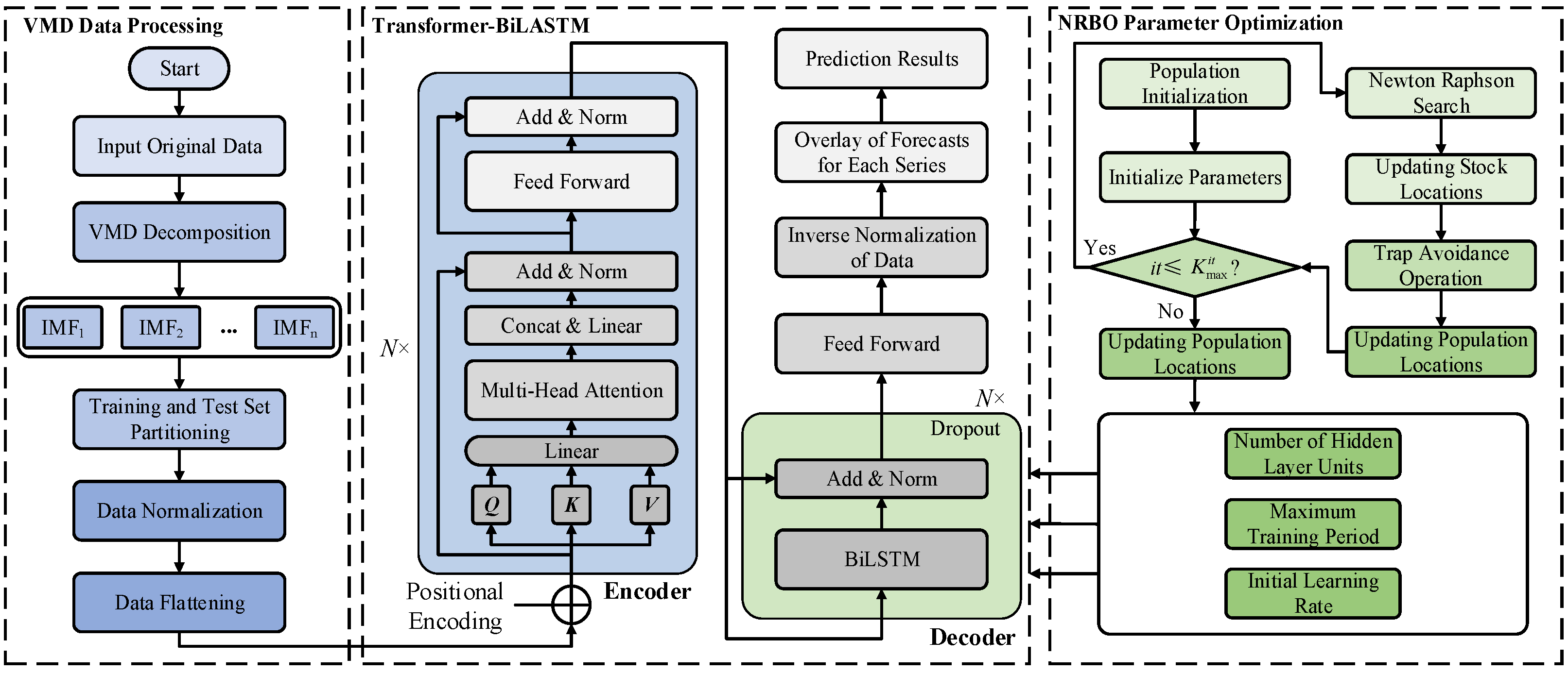
5. VMD-NRBO-Transformer-BiLSTM Hybrid Prediction Model

5.1. Optimization of Model Parameters

The Transformer–BiLSTM network model contains numerous hyperparameters, such as the number of training epochs, the number of hidden units in the layers, the learning rate, and regularization parameters, all of which significantly affect the model’s training performance. Manually selecting these hyperparameters is a complex and time-consuming process, and conventional experience-based methods may not be effective across different prediction scenarios. To address this, the NRBO algorithm is employed in this paper to optimize the selection of hyperparameters, specifically targeting the number of hidden units, the maximum number of training epochs, and the initial learning rate. Additionally, the Adam optimizer is used to adaptively adjust the learning rate for each parameter, thereby accelerating convergence and enhancing overall model performance.

5.2. Overall Framework

The overall framework of the VMD-NRBO-Transformer-BiLSTM hybrid network model is illustrated in Figure 5. The model consists of three primary modules. First, the raw data are processed using VMD, which decomposes the data into multiple subsequences. These subsequences are then split into training and testing sets. Next, the data undergo normalization and flattening before being input into the Transformer–BiLSTM network for model training and testing. The predicted values for each subsequence are subsequently re-denormalized and combined to yield the final prediction. Simultaneously, the NRBO algorithm is employed to optimize the model’s initial hyperparameters, thereby enhancing its prediction accuracy.

In summary, the prediction model proposed in this paper provides a good solution in terms of input data feature acquisition, solving the long-term dependency and gradient explosion of time-series data, and the problem of hyperparameter selection for network models. The denoising of nonlinear complex signals is realized by using the VMD technique, the combination of BiLSTM and Transformer makes Transformer more adept at dealing with the prediction of time-series data, and the introduction of the NRBO algorithm makes the hyperparameter selection of the network model more suitable to the predicted data features and improves the model’s training effect.

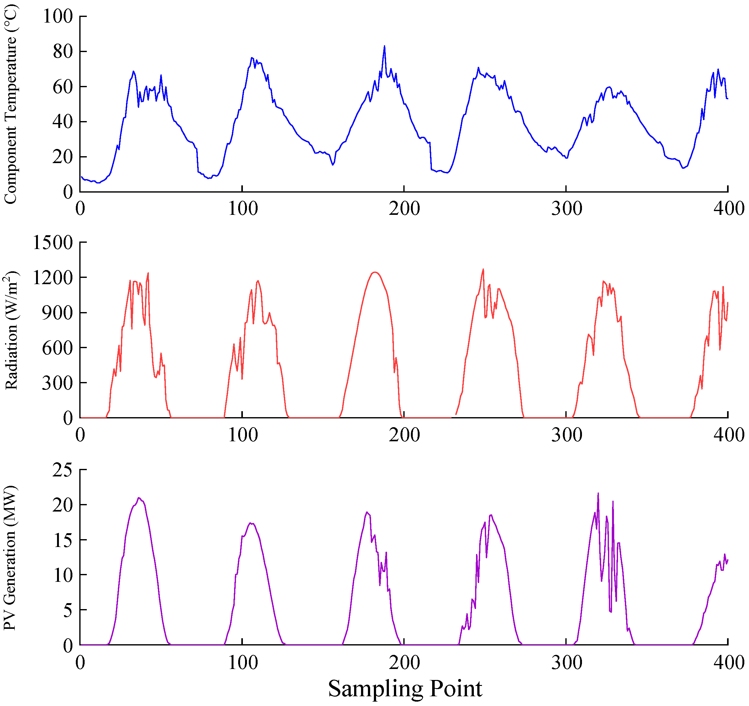
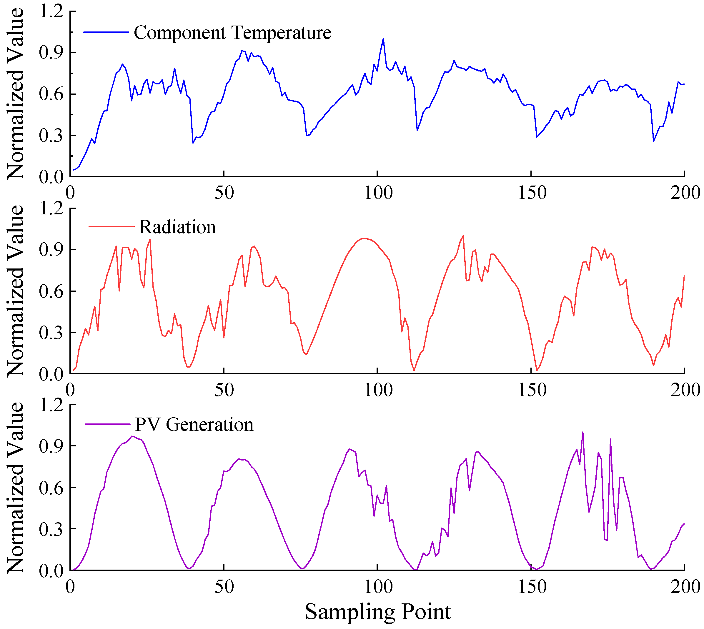
6. Example Analysis

This paper uses field data from a photovoltaic power generation system in a northern city in China, recorded in 2019, as the experimental dataset for model simulation. The dataset includes historical meteorological data and photovoltaic output data, with a sampling interval of 20 min. The first 70% of the dataset is allocated as the training set, while the remaining 30% is used as the testing set for model training and evaluation.

6.1. Parameter Settings

The hyperparameter settings for the NRBO algorithm and the optimized network model are provided in

Table 1. Model parameter settings.

Parameter	Value
Population Size	3
$\mathrm{Maximum}\mathrm{Number}\mathrm{of}\mathrm{Iterations}{K}_{\max }^{i\mathit{t}}$	20
Optimization Lower Bound lb	[50, 50, 0.001]
Optimization Upper Bound	[300, 300, 0.01]
Number of Attention Heads	4
Dropout	0.2
Number of Hidden Layer Units	204
Epoch	300
Initial Learning Rate	0.0087
Regularization Coefficient	0.001

.

6.2. Model Evaluation Metrics

This paper employs five evaluation metrics to assess the model’s prediction accuracy: Mean Absolute Error (MAE), Mean Squared Error (MSE), Root Mean Squared Error (RMSE), Mean Absolute Percentage Error (MAPE), and Coefficient of Determination (R²).

$$MAE={\displaystyle \frac{{\displaystyle \sum _{i=1}^n\left|{\widehat{y}}_i-y_i\right|}}{n}}$$

(32)

$$MSE={\displaystyle \frac{{\displaystyle \sum _{i=1}^n{\left({\widehat{y}}_i-y_i\right)}^2}}{n}}$$

(33)

$$RMSE=\sqrt{{\displaystyle \frac{{\displaystyle \sum _{i=1}^n{\left|{\widehat{y}}_i-y_i\right|}^2}}{n}}}$$

(34)

$$MAPE={\displaystyle \frac{1}{n}}{\displaystyle \sum _{i=1}^n\left|\frac{{\widehat{y}}_i-y_i}{y_i}\right|}$$

(35)

$$R^2=1-{\displaystyle \frac{{\left({\widehat{y}}_i-y_i\right)}^2}{{\displaystyle \sum _{i=1}^n{\left(\overline{y}-y_i\right)}^2}}}$$

(36)

Here, $y_i$ is the actual photovoltaic output value, ${\widehat{y}}_i$ is the predicted photovoltaic output value, $\overline{y}$ is the mean of the actual photovoltaic output samples, and n is the number of samples. The smaller the values of the MAE, MSE, RMSE, and MAPE, the closer R² is to 1, indicating higher model prediction accuracy. If R² > 0.4, the model fitting is considered to be good.

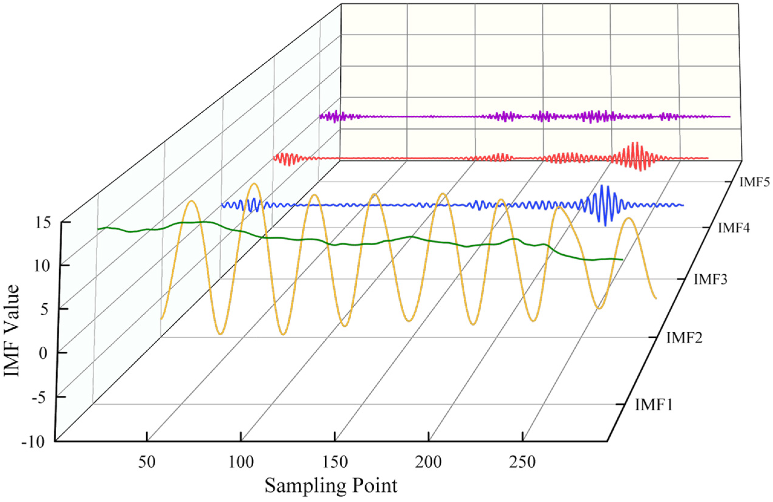
6.3. Decomposition of Original Data

The input historical data contain module temperature, radiance, and PV output data, some of which are shown in Figure 6. Due to the intermittent nature of PV output, there are many zero values in the data, and there will be an infinite number of outliers when calculating the MAPE value, so the points in the dataset where the PV output is zero are eliminated. And because there are some differences in the number of units and orders of magnitude between different feature quantities, the direct input into the model will have an impact on the model training effect, so first of all, we need to normalize the dataset, mapping to the [0, 1] range.

$${\mathit{X}}_{\mathrm{normlized}}={\displaystyle \frac{{\mathit{X}}_i-{\mathit{X}}_{\min }}{{\mathit{X}}_{\max }-{\mathit{X}}_{\min }}}$$

(37)

Here, ${\mathit{X}}_{\mathrm{normlized}}$ represents the normalized value. ${\mathit{X}}_{\max }$ and ${\mathit{X}}_{\min }$ are the maximum and minimum values of the input features, respectively. ${\mathit{X}}_i$ is the i-th value of the input feature. The distribution of certain original input features and photovoltaic output data after normalization is illustrated in Figure 7.

The photovoltaic power generation time series exhibits characteristics such as nonlinearity and volatility, which increase the complexity of predictions when directly input into the model. The data are also highly susceptible to noise, further affecting prediction accuracy. To address these issues, after removing zero values from the original photovoltaic output data, VMD is applied. The second-order penalty factor $\alpha$ of the VMD optimized by GWO is 2376, and the modal number K is 5, resulting in five photovoltaic subsequence datasets. A portion of the resulting waveforms is presented in Figure 8.

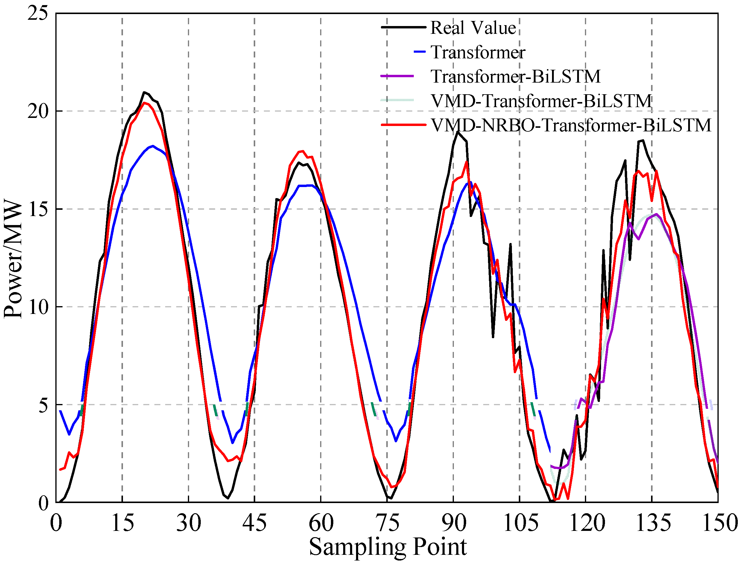
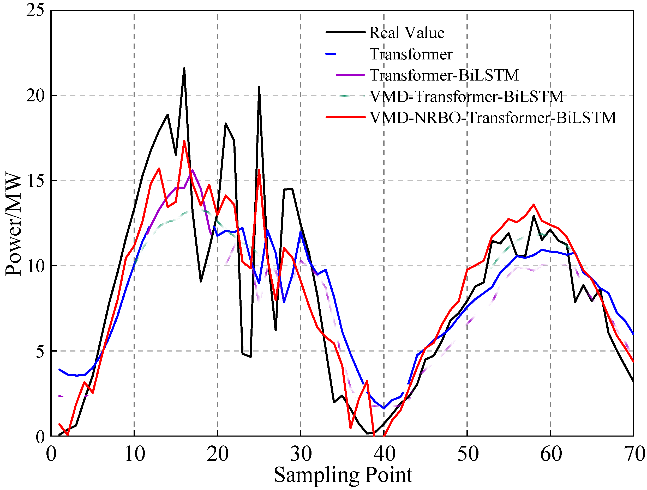
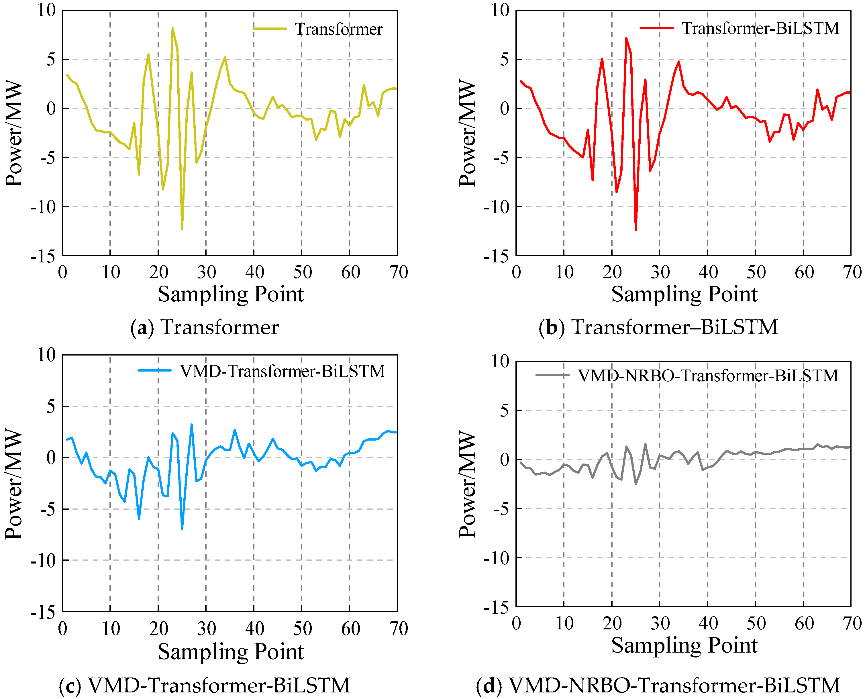
6.4. Comparison and Analysis of Prediction Results

To assess the accuracy of the model proposed in this study, a comparative analysis is conducted between the proposed model and three other prediction models: Transformer, Transformer–BiLSTM, and VMD-Transformer-BiLSTM. The same dataset is utilized for both model training and testing, and error analysis is performed on the results from both phases.

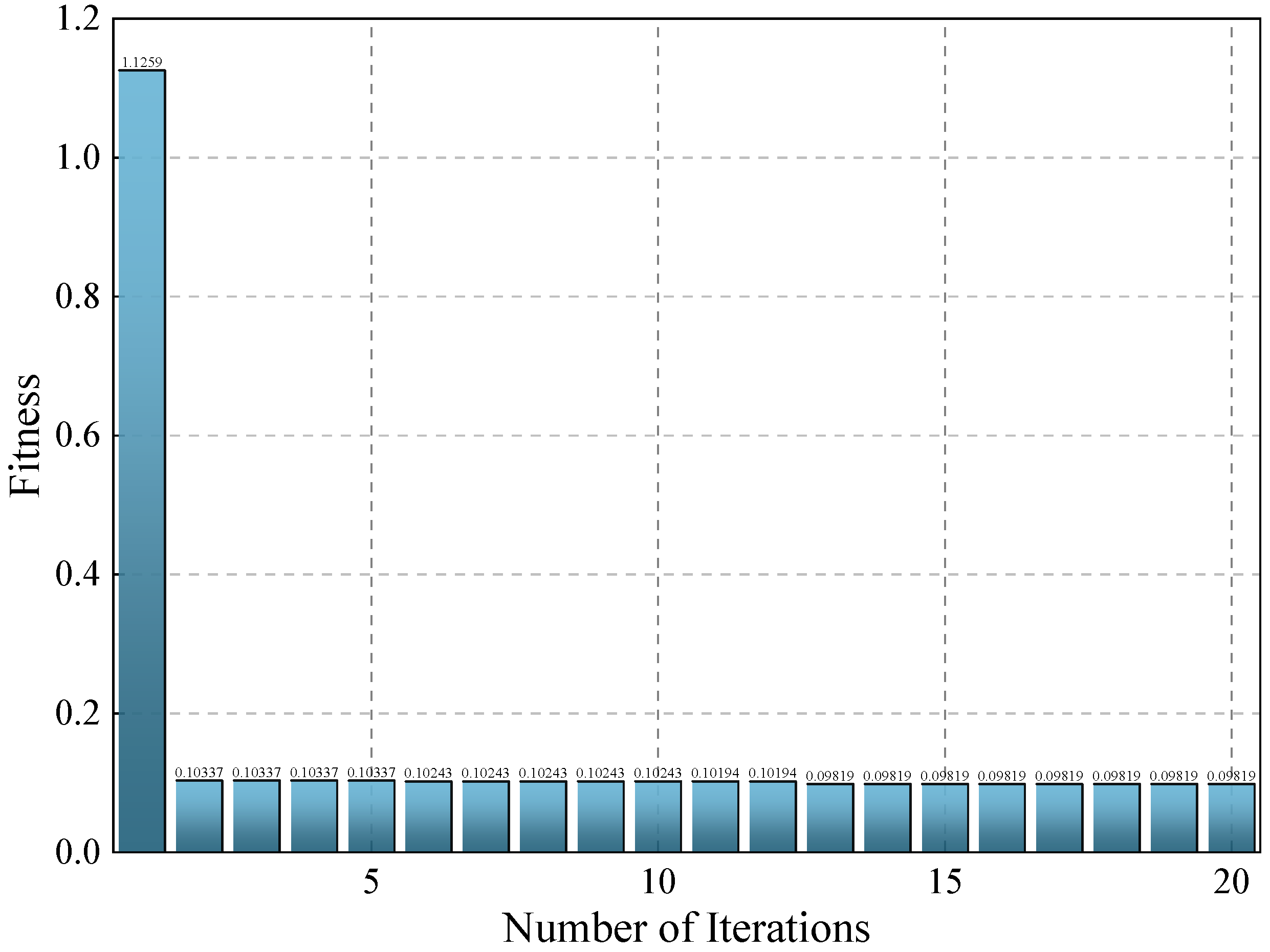
6.4.1. Iterations of the NRBO Algorithm

The iteration curve of the NRBO algorithm is presented in Figure 9. As shown in the figure, the algorithm approaches the convergence value after the second iteration and reaches convergence at the 13th iteration, with the fitness value stabilizing at 0.09819.

6.4.2. Comparison of Training and Test Results

The training effect of each model on the training set is given in Figure 10, which shows 150 data points of the training set as well as the training results of each model. And as far as is observed in the figure, it is known that the training effect of the VMD-NRBO-Transformer-BiLSTM model significantly outperforms that of the Transformer, Transformer–BiLSTM, and VMD-Transformer-BiLSTM models, especially at the peak PV output, which is closer to the real curve.

Figure 11 illustrates the prediction performance of each model on the test set, based on the results from 70 sampling points. The solution times of the four models for the test set are 3.64 s, 4.21 s, 4.52 s, and 4.46 s, respectively. As shown in the figure, the overall prediction curve of the VMD-NRBO-Transformer-BiLSTM model closely aligns with the actual curve. This model effectively captures the fluctuations in the output, demonstrating superior accuracy in simulating the volatility of photovoltaic output.

Figure 12 illustrates the error distribution between the predicted and actual values for the four models on the test set.

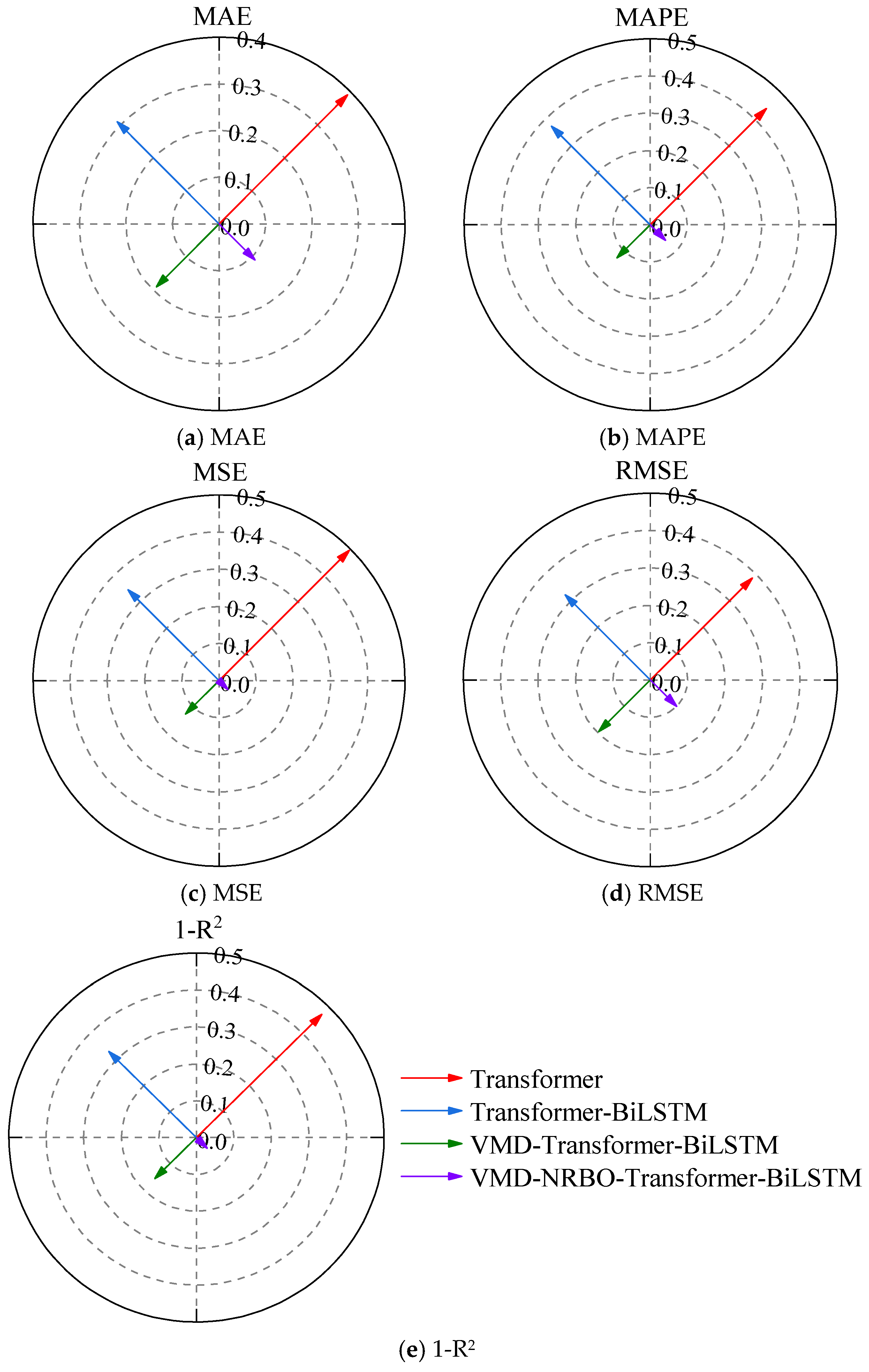
6.4.3. Comparison of Evaluation Metrics

The error evaluation metrics for each prediction model were computed based on the test results from the test set.

Table 2. Evaluation metric results of each model.

Model	MAE	MAPE	MSE	RMSE	R2
Transformer	3.160	1.503	15.471	3.933	0.486
Transformer–BiLSTM	2.501	1.276	10.793	3.285	0.641
VMD-Transformer-BiLSTM	1.536	0.427	3.960	1.990	0.830
VMD-NRBO-Transformer-BiLSTM	0.885	0.199	1.032	1.016	0.956

provides a summary of the error evaluation metrics for all the models.

Compared with the single Transformer model, the Transformer–BiLSTM model improves the Transformer decoder part to BiLSTM on this basis, which solves the long-term dependency problem in the input sequence data, and the bidirectional data processing makes the message acquisition more comprehensive. The MAE, MAPE, MSE, and RMSE are reduced by 20.85%, 15.10%, 30.24%, and 16.48%, and the R2 increases by 31.89%. It can be seen that the R² of all four models is greater than 0.4, and all of them have good fitting effect.

Compared with the Transformer–BiLSTM model, the VMD-Transformer-BiLSTM model adds the VMD on the basis of this model, removes the redundant noise signals in the original data, and retains the key information, which optimizes the prediction effect. The MAE, MAPE, MSE, and RMSE are reduced by 38.58%, 66.54%, 63.31%, and 39.42%, and the R² increased by 29.49%.

The various error evaluation indexes of the VMD-NRBO-Transformer-BiLSTM model are optimal among all models, compared with the VMD-Transformer-BiLSTM model, and the NRBO algorithm is added, which is a reasonable optimization for the initial hyperparameters of the network model, and it improves the efficiency of the model training and the prediction accuracy. The MAE, MAPE, MSE, and RMSE were reduced by 42.38%, 53.40%, 73.94%, and 48.94%, respectively, and the R² increased by 15.18%.

To visually illustrate the differences in the error evaluation metrics across the models and emphasize the advantages of the VMD-NRBO-Transformer-BiLSTM model, the evaluation metric results are presented in compass diagrams. Prior to plotting, the values are normalized to a common scale, and each value is represented as a proportion of the total sum for the corresponding metric. The compass diagrams depicting the error evaluation metrics are shown in Figure 13.

Combining the results of the above studies, the VMD-NRBO-Transformer-BiLSTM prediction model proposed in this paper provides a good solution to the problems of input data feature acquisition, capturing long-term dependencies and gradient explosions of time-series data, as well as network model hyperparameter selection. In previous studies, the volatility and nonlinearity of PV output data make prediction difficult, and the denoising of nonlinear complex signals using the VMD technique removes signal redundancy and retains key information. The combination of BiLSTM and Transformer makes Transformer more adept at handling the prediction of time-series data and improves the information capturing ability. Previously, model hyperparameter selection relied on human experience, and the introduction of the NRBO algorithm makes the hyperparameter selection of the network model more suitable for the predicted data features.

7. Conclusions

In this paper, a VMD-NRBO-Transformer-BiLSTM short-term PV output prediction model is proposed for the PV output uncertainty problem. Through example tests, the model has better error evaluation indexes and better prediction effects than the general Transformer model, the Transformer model incorporating BiLSTM, and the Transformer–BiLSTM model utilizing VMD. The following conclusions are drawn:

• The VMD method effectively mitigates the challenge of feature extraction caused by the volatility of photovoltaic output data. By removing high-frequency components from each decomposed mode and reconstructing the data using the remaining components, the resulting waveform becomes smoother while preserving key information. This process effectively filters out noise, thereby reducing its interference with the model’s predictions.
• Building on the Transformer encoder–decoder architecture, BiLSTM is employed to replace the attention layer in the original Transformer decoder, while residual connections are introduced to process the input sequence data. This approach preserves the encoder’s information, enhances the model’s capacity to capture and process relevant features, and effectively addresses the challenge of long-term dependencies in sequence data.
• The NRBO algorithm overcomes the challenges associated with manually selecting hyperparameters for the network model, as well as the limitations of empirical selection methods in specific prediction scenarios. As a result, the model’s prediction accuracy is significantly enhanced. The MAE, MAPE, MSE, and RMSE are reduced by 42.38%, 53.40%, 73.94%, and 48.94%, respectively, while the R² score increases by 15.18%.

In addition, this paper only focuses on the accuracy of PV power generation prediction over the past few days. It has not yet considered the training of the model and prediction solving efficiency, as real-time fast prediction has not been further studied, and has not been further divided into prediction scenarios, which cannot guarantee the prediction effect of different weather and regions. It can be used to perform in-depth research on the universality of model application and real-time prediction in the future.

Finally, for microgrid system operators, selecting a good prediction model, combining the advantages of each network and algorithm, and selecting the local PV output historical data for a large number of model training allows the prediction model to be deployed in advance to accurately predict distributed PV output, which is conducive to the accurate formulation of the microgrid scheduling plan.

References

- Liu, H.; Shi, Y.; Guo, L.; Qiao, L. China’s energy reform in the new era: Process, achievements and prospects. J. Manag. World 2022, 38, 6–24. [Google Scholar]
- Zhu, Q.; Li, J.; Qiao, J.; Shi, M.; Wang, C. Application and prospect of artificial intelligence technology in renewable energy forecasting. Proc. CSEE 2023, 43, 3027–3047. [Google Scholar]
- Hu, Z.; Gao, Y.; Ji, S.; Mae, M.; Imaizumi, T. Improved multistep ahead photovoltaic power prediction model based on LSTM and self-attention with weather forecast data. Appl. Energy 2024, 359, 122709. [Google Scholar] [CrossRef]
- Yu, Z. Transformer-Based Photovoltaic Power Generation Prediction Method for Long Sequences. Nanchang University, Nanchang, China, 2024. [Google Scholar]
- Chen, Y.; Ma, X.; Cheng, K.; Bao, T.; Chen, Y.; Zhou, C. Ultra-short-term power forecast of new energy based on meteorological feature selection and SVM model parameter optimization. Acta Energiae Solaris Sin. 2023, 44, 568–576. [Google Scholar]
- Zhong, A.; Wu, Z.; Xie, Z.; Mao, Y.; Yang, L. Research on short-term power prediction of photovoltaic power generation based on ACO-BP neural network. Electron. Des. Eng. 2024, 32, 82–86. [Google Scholar]
- Zhang, B.; Wang, X.; Zhou, W.; Chen, Z.; Wang, J. Photovoltaic power generation prediction based on machine learning taking Jinhua City as an example. Technol. Mark. 2022, 29, 17–22. [Google Scholar]
- López Santos, M.; García-Santiago, X.; Echevarría Camarero, F.; Blázquez Gil, G.; Carrasco Ortega, P. Application of temporal fusion transformer for day-ahead PV power forecasting. Energies 2022, 15, 5232. [Google Scholar] [CrossRef]
- Zhu, H.; Sun, Y.; Zhou, H.; Guan, Y.; Wang, N.; Ma, W. Intelligent clustering-based interval forecasting method for photovoltaic power generation using CNN-LSTM neural network. AIP Adv. 2024, 14, 065329. [Google Scholar] [CrossRef]
- Cao, Y.; Liu, G.; Luo, D.; Bavirisetti, D.P.; Xiao, G. Multi-timescale photovoltaic power forecasting using an improved Stacking ensemble algorithm based LSTM-Informer model. Energy 2023, 283, 128669. [Google Scholar] [CrossRef]
- Zhang, C.; Peng, T.; Nazir, M.S. A novel integrated photovoltaic power forecasting model based on variational mode decompo-sition and CNN-BiGRU considering meteorological variables. Electr. Power Syst. Res. 2022, 213, 108796. [Google Scholar] [CrossRef]
- Dragomiretskiy, K.; Zosso, D. Variational Mode Decomposition. IEEE Trans. Signal Process. 2014, 62, 531–544. [Google Scholar] [CrossRef]
- Yanovsky, I.; Dragomiretskiy, K. Variational destriping in remote sensing imagery: Total variation with L1 fidelity. Remote Sens. 2018, 10, 300. [Google Scholar] [CrossRef]
- Ma, K.; Nie, X.; Yang, J.; Zha, L.; Li, G.; Li, H. A power load forecasting method in port based on VMD-ICSS-hybrid neural network. Appl. Energy 2025, 377, 124246. [Google Scholar] [CrossRef]
- Wang, F.; Wang, S.; Zhang, L. Ultra short term power prediction of photovoltaic power generation based on VMD-LSTM and error compensation. Acta Energiae Solaris Sin. 2022, 43, 96–103. [Google Scholar]
- Yu, Y.; Shekhar, A.; Chandra Mouli, G.R.; Bauer, P. Comparative impact of three practical electric vehicle charging scheduling schemes on low voltage distribution grids. Energies 2022, 15, 8722. [Google Scholar] [CrossRef]
- Mirjalili, S.; Mirjalili, S.M.; Lewis, A. Grey Wolf Optimizer. Adv. Eng. Softw. 2014, 69, 46–61. [Google Scholar]
- Li, J.; Du, J.; Zhu, Y.; Guo, Y. Survey of Transformer-based object detection algorithms. Comput. Eng. Appl. 2023, 59, 48–64. [Google Scholar]
- Zhang, X. Semantic Relation Extraction Method Based on Bidirectional Encoder Representations from Transformers. Henan University, Kaifeng, China, 2021. [Google Scholar]
- Lu, W.; Li, J.; Wang, J.; Qin, L. A CNN-BiLSTM-AM method for stock price prediction. Neural Comput. Appl. 2021, 33, 4741–4753. [Google Scholar]
- Ren, J.; Wei, H.; Zou, Z.; Hou, T.; Yuan, Y.; Shen, J.; Wang, X. Ultra-short-term power load forecasting based on CNN-BiLSTM-Attention. Power Syst. Prot. Control 2022, 50, 108–116. [Google Scholar]
- Qin, Q.; Lai, X.; Zou, J. Direct multistep wind speed forecasting using LSTM neural network combining EEMD and fuzzy entropy. Appl. Sci. 2019, 9, 126. [Google Scholar] [CrossRef]
- Liu, T.; Liu, S.; Heng, J.; Gao, Y. A new hybrid approach for wind speed forecasting applying support vector machine with ensemble empirical mode decomposition and cuckoo search algorithm. Appl. Sci. 2018, 8, 1754. [Google Scholar] [CrossRef]
- Li, Y.; Shi, G.; Liao, Y.; Li, J.; Chen, X.; Huang, W. Research on monthly runoff prediction based on NRBO-SVM model. Water Power 2024, 1–7. Available online: https://link.cnki.net/urlid/11.1845.TV.20240808.1430.007 (accessed on 4 December 2024).
- Weerakoon, S.; Fernando, T. A variant of Newton’s method with accelerated third-order convergence. Appl. Math. Lett. 2000, 13, 87–93. [Google Scholar] [CrossRef]
- Argyros, I.K.; Magreñán, Á.A. Iterative Methods and Their Dynamics with Applications: A Contemporary Study; CRC Press: Boca Raton, FL, USA, 2017. [Google Scholar]
- Ahmadianfar, I.; Bozorg-Haddad, O.; Chu, X. Gradient-based optimizer: A new metaheuristic optimization algorithm. Inf. Sci. 2020, 540, 131–159. [Google Scholar] [CrossRef]