Article

Exploration of Machine Learning Models for Prediction of Gene Electrotransfer Treatment Outcomes

1
Department of Medical Engineering, University of South Florida, Tampa, FL 33620, USA
2
Department of Orthopedic Surgery, Morsani College of Medicine, University of South Florida, Tampa, FL 33620, USA
*
Author to whom correspondence should be addressed.
Appl. Sci. 2024, 14(24), 11601; https://doi.org/10.3390/app142411601
Submission received: 1 November 2024 / Revised: 2 December 2024 / Accepted: 9 December 2024 / Published: 12 December 2024

Abstract

:
Gene electrotransfer (GET) is a physical method of gene delivery to various tissues utilizing pulsed electric fields to transiently permeabilize cell membranes to allow for genetic material transfer and expression. Optimal pulsing parameters dictate gene transfer efficiency and cell survival, which are critical for the wide adaptation of GET as a gene therapy technique. Tissue heterogeneity complicates the delivery process, requiring the extensive optimization of pulsing protocols currently empirically optimized. These experiments are time-consuming and resource-intensive, requiring large numbers of animals for in vivo optimization. Advances in machine learning (ML) and computing power, data analysis, and model generation using ML techniques, such as neural networks, enable predictive modeling for GET. ML models have been used previously to predict ablation performance in irreversible electroporation procedures and single-cell electroporation platforms. In this work, we present ML predictive models that could be used to optimize pulsing parameters based on already completed experiments. The models were trained on 132 data points from 19 papers with the Matlab Statistics and Machine Learning Toolbox. An artificial neural network (ANN) was generated that could predict binary treatment outcomes with an accuracy of 71.8%. Support vector machines (SVMs) using selected features based on χ 2 tests were also explored. All models used a maximum of 24 features as input, spread across target species, needle configuration, pulsing parameters, and plasmid parameters. Pulse voltage and pulse width dominated as the critical parameters, followed by field strength, dose, and electrode with the greatest impact on GET efficiency. This study elucidates areas where predictive ML algorithms may ideally inform GET study design to accelerate optimization and improve efficiencies upon the further training of these models.

1. Introduction

Gene transfer, and the resulting expression of the encoded protein, has been used for decades in the treatment of disease, as well as for improvements in quality of life for those with genetic disorders [1]. There are several well-known methods for the delivery of genetic material: viral, physical, and nanoparticle-based. In the domain of physical transfection technologies, gene electrotransfer (GET) has become popular as an effective and relatively safe way to deliver genetic material to target tissues [2]. GET involves the use of pulsed electric fields (PEFs) to facilitate the transfer of exogenous genetic material, typically naked plasmid DNA, through the cell membrane to be translated by the host cell into a therapeutically useful protein [3,4]. A typical treatment involves the injection of the plasmid DNA, followed by the direct application of the prescribed PEFs to the desired tissue. The actual shape, magnitude, repetition rate, and count of these PEFs varies dependent on the plasmid DNA used, tissue to be treated, and physical configuration of the electrode used to deliver them [5,6].
Gene transfer efficiency and resulting protein expression are highly dependent on selecting proper pulsing parameters and resulting electric fields [6]. Applying GET to various tissues in the body has also shown that expression is highly dependent on intrinsic tissue properties and, thus, no universal approach exists to date [7]. These parameters, both electrical and biological, have been the focus of previous, empirical optimization efforts.
In the case of electrical parameters, the number of pulses, pulse width, applied voltage, repetition rate, and electrode configuration determine the magnitude, direction, and distribution of electric fields in the treated tissue. By changing any of these parameters, the amount and distribution of electrical energy delivered to the tissue can be modulated. These effects have been shown by modeling the underlying processes through the finite element modeling (FEM) of tissues, pulses, and electrode configurations [8,9,10], and the impact of changing these parameters has been shown in empirical optimization studies [11,12].
There is a delicate balance between efficiently and transiently permeabilizing cells within tissues and overpulsing [13]. Overpulsing leads to permanent damage to cell membranes resulting in cell death, which is undesirable for gene therapy applications and enters the field of irreversible electroporation (IRE) or electrical ablation. Underpulsing, on the other hand, results in reduced cell permeabilization and insufficient or zero gene transfer efficiency [6,14,15].
Electrical parameters are not the only variables impacting the efficacy of gene electrotransfer success. Biological parameters such as tissue characteristics and the size of the plasmid DNA used can impact treatment success. Specific tissues under treatment, such as skin, muscles, or tumors, all have varying electrical properties that can greatly impact the distribution of electric fields during treatment [16]. Similarly, tissue impedance was found to change as a GET treatment progressed [17,18,19,20], and these changes were not identical across all tissue types [21]. Thus, electric field distributions change as GET treatment progresses, depending on the underlying tissue type. Regarding the size of the plasmid DNA used, plasmid DNA with larger backbones was found to decrease transfection efficiency when compared to plasmid DNA with smaller backbones [5]. So, despite ultimately expressing the same protein, the smaller plasmid DNA allowed for higher transfection efficiency despite the same electrical parameters being used.
Since the first treatments in the 1980s, the optimization of GET protocols has been an experimentally intensive endeavor. These experiments require large numbers of animals, usually mice, rats, and guinea pigs, but also validation in large animals such as pigs prior to progression to clinical trials. Despite this, successful GET protocols have been established in various tissues empirically, including the development of GET-mediated interleukin-12 (IL-12) delivery to melanoma with successful phase I and phase II clinical trials, indicating that plasmid DNA delivery encoding IL-12 can stimulate the immune system to clear treated lesions and metastatic disease [22,23]. While there have been major advancements in pulse type, electrode design [24,25,26], external stimuli such as heat [27,28], and real-time treatment endpoint detection using impedance [20,29,30], the underlying problem of searching the vast parameter space remains.
Machine learning models have been in use for many years but, due to the recent increases in computing power, have found more mainstream accessibility and acceptance. Models have been applied to diagnostic image processing in radiology [31] and histological imaging [32] and in adverse event detection using respiratory data [33]. Machine learning models have also been applied to the field of electroporation, specifically artificial neural networks (ANNs) for IRE [34,35], support vector machines (SVMs) for interpreting post-ablation outcomes from magnetic resonance imaging (MRI) [36], and fully convolutional networks (FCNs) and computer vision for the identification of potential tumors to treat using a multi-electrode structure [37]. In the field of GET, machine learning has only been used to locate cells using computer vision for the application of targeted, single-cell therapies [38] or in in vitro studies limited to single cell lines [39]. To date, the prospect of applying these techniques to GET on a tissue scale remains elusive.
A complicating factor to the development and deployment of such a machine learning model is that there is no standard for the reporting of pulsing parameters across different studies and no existing repository or database for documenting pulsing parameters and resulting tissue responses. While the methodologies used in reporting are varied, the related parameters can often be translated from one lab to another, such as how some labs report the time between pulses or a pulse frequency, which both effectively describe the same thing. However, this introduces the possibility of errors in translation or misinterpretation of the intention behind the way in which these values are reported. A standardized method would avoid such potential errors and allow for the rapid creation of datasets where all necessary parameters are reported in a uniform way, avoiding the need for translation or interpretation.
ANNs were the first choice for the models as they are extremely customizable and flexible when dealing with variable input data types and have been successfully employed in similar endeavors in the field of IRE [34,35]. However, they suffer from a need for large datasets to effectively predict outcomes. This need grows exponentially as the number of features, or data categories, increases [40]. Since the data available are relatively limited and have a comparatively large number of features, SVMs were chosen as a second option as they are capable of accurate predictions with more limited sample sizes compared to ANNs [41].
This paper presents an exploratory study on the application of two machine learning models to a dataset of GET experiments published over the course of the last 30 years.

2. Materials and Methods

2.1. Paper Selection and Data Curation

The initial literature search for papers for inclusion in the dataset was limited based on whether the papers
  • conducted GET experiments with PEFs and plasmid DNA;
  • did not use additional therapeutic techniques to achieve success;
  • used a pulse configuration with a maximum of two separate voltage levels;
  • provided results in terms of significant difference from the control;
  • conducted experiments either in vitro or in vivo.
The data from the papers were then manually captured in a spreadsheet using the features described in Table 1.
For training inputs, electrode configurations and electrode types were labeled based on the descriptions provided in the source papers. Electrode types were split into either penetrating or non-penetrating electrodes, where penetrating electrodes were intended to pierce the target tissue and non-penetrating electrodes were intended to rest on the surface. In vitro studies were classed as non-penetrating electrodes due to the use of cuvettes and plate electrodes in their methodologies.
The features Specific Tissue and Tissue as well as Specific Species and Species were added to avoid overspecification of the experimental targets. The inclusion of both features allowed the learning algorithms to decide if a particular outcome was better predicted by a general species/tissue designation rather than the specific tissue or species under study (e.g., ‘Tumor’ vs. ‘B16 Melanoma’ or ‘Rat’ vs. ‘Sprague Dawley Rat’).
It was often the case that either the voltage or the field strength was not directly reported. However, if the paper included the relevant electrode spacings, the missing value was calculated using
E = V/d,
where E is the electric field strength in V/cm, V is the applied voltage in V, and d is the electrode spacing in cm. While this does not provide an accurate representation of the field strength between electrodes, it is commonly used in the field to relate the applied voltage and expected field strengths when reported in the literature [25,42,43,44].
In the case of the monopolar electrodes [45], the method of determining the field strength directly from the parameters and geometries reported in the papers was not possible as the grounding electrode was significantly distant from the active electrode. In this case, COMSOL FEM simulations were employed to simulate the field strengths proximal to the active electrode during pulsing. Geometries and tissue types were determined from the papers, whereas the electrical properties of the tissues of interest were determined based on electrical parameters described in [16].
Sex was handled using four potential variables: Male, Female, M/F, and NP. M/F was used in cases where the group under study was a mix of male and female animals but the results and conclusions were not separated by sex. NP was used for one study where the sex of the animals was not provided. Sex and species for in vitro studies were entered based on the sex and species of the source of the cells under study.
In cases where the pulse parameters denoted only one voltage, all the dual features (V1/V2, Field Strength 1/2, etc.) were filled with the same information. For studies where the pulse parameters did vary within a pulse train, the first set of parameters always corresponded to the parameters of the first pulse in the train. All voltages and field strengths were entered as positive values, with pulse polarity accounting for any positive to negative voltage transitions. In cases where pulse frequency was reported instead of the time between pulses, the time between pulses was calculated as the inverse of the pulse frequency.
The outcome of each referenced study varied depending on both the goal of the study and the plasmid used to achieve said goal. These outcomes ranged from the amount of protein expression to patient outcomes in clinical trials. Due to the variability of the biological responses reported in the literature, the outcomes of the studies were entered as a binary variable rather than entering the outcome data from the papers directly. This binary classification allowed the models to report either a ‘success’ or ‘fail’, rather than dynamically predicting gene transfection efficiencies or patient outcomes based on the goal of the study. In the case of human cancer trials, success was considered as either stable disease or a complete response, whereas failure was considered in the case of progressive disease. In all other cases, success was considered a statistically significant improvement in the biological responses between the test group and a fixed control. In the event that a particular paper had multiple reported experiments, of which only a portion conformed to the requirements for inclusion in the dataset, only the relevant experiments were included in the dataset.

2.2. Determination of the Most Important Features

χ 2 tests were conducted between each feature and the binary outcome variable. The features were then sorted by the respective p-value, with lower p-values being ranked more highly. SVMs were trained on limited feature sets of 5, 6, 7, 8, and 9 features, informed by the results of the χ 2 tests, to determine if using limited feature sets improved model outcomes. The process of training ANNs should include weighing features with the greatest impact on the outcome, but training with the limited datasets was performed with the ANNs as well for exploratory purposes. Reducing the number of features available to the ANN models had the potential to offset the need for the large datasets discussed in Section 2.2.
To validate the ranking of predictor variables, the above χ 2 tests were carried out 100 times with randomized subsets of data containing 70% of the source dataset. The resulting rankings were then plotted with 95% confidence intervals to determine if the rankings were independent of individual samples.

2.3. Training of the Machine Learning Models

The 132 experiments were split into two datasets: one for training and one for testing; 70% of the data was used in training, while the remaining 30% was used in the test set. The ratio between significant and non-significant outcomes was maintained in both the training and test sets.
In the case of the SVM models, six total models were trained. The ‘basic’ SVM model was trained on a subset of data containing all predictors. The remaining five SVM models were trained on a further limited subset of the data containing the top 5, 6, 7, 8, and 9 predictors. The top predictors were determined using the χ 2 tests described in Section 2.2.
Eight ANN models were trained targeting different optimization techniques. The first model was trained using a default ANN, with one layer of width 10, a rectified linear unit (ReLU) activation function, and standardized feature inputs. A second ANN was trained by adjusting the regularization strength, λ , while minimizing cross-validation classification error. The value of λ corresponding to the minimum cross-validation classification error was then used in the final model. The third ANN was subjected to an expected improvement in the Bayesian optimization procedure to discover optimal parameters, while avoiding overfitting the model to the training data. The optimizer was allowed to adjust layer number, layer width, activation function, and regularization strength. The ‘basic’, ‘ λ -optimized’, and ‘hyperparameter-optimized’ ANN models were trained with access to all predictors in the 70% training set. The remaining five ANN models were trained using the previously mentioned default parameters but on limited datasets of the 5, 6, 7, 8, and 9 most important features as determined by the χ 2 testing described in Section 2.3.

2.4. Assessing the Accuracy of the Models

In all cases, a confusion matrix was generated for each of the 14 models comparing predicted outcomes from the models to the true labeled data from the test dataset. Several figures of merit were calculated based on the confusion matrix [46]: accuracy, sensitivity, specificity, F1-score, Matthews correlation coefficient (MCC), and receiver operator characteristic (ROC) area under the curve (AUC).
Accuracy is effectively a measure of generally how often a model is correct in its predictions considering both positive and negative predictions. Accuracy was determined as the ratio of the sum of true positive (TP) and true negative (TN) predictions to the total number of samples in the test set. Sensitivity is a measure of the accuracy of a model only regarding positive predictions and was calculated as the ratio of the true positive predictions to the total number of actual positives in the data. Specificity is the same as sensitivity, except only regarding negative predictions. It was calculated in a similar manner as the ratio of true negative predictions to the total number of actual positives in the data. The calculations are summarized below:
A c c u r a c y = T P + F P T P + F P + T N + F N ,
S e n s i t i v i t y = T P T P + F N ,
S p e c i f i c i t y = T N T N + F P ,
Two general goodness-of-fit measures were considered for this study: F1-score and MCC. The F1-score is a harmonic average of precision and recall, while the MCC is a more robust measure of classification models trained on unbalanced datasets, where the two classifications are not equally represented [46]. In this case, the data contain a larger proportion of significant results versus non-significant results. The F1-score ranges from 0 to 1 (0 being worst), with a value of 0.5 being equal in effectiveness to a coin-flip predictor. The MCC score ranges from −1 to 1 (−1 being worst), with an MCC of 0.3 being considered acceptable and an MCC of 0 representing the coin-flip predictor [46]. The two measures were calculated as follows:
F 1 = 2 T P 2 T P + F P + F N ,
M C C = T P T N F P F N T P + F P T P + F N T N + F P T N + F N ,
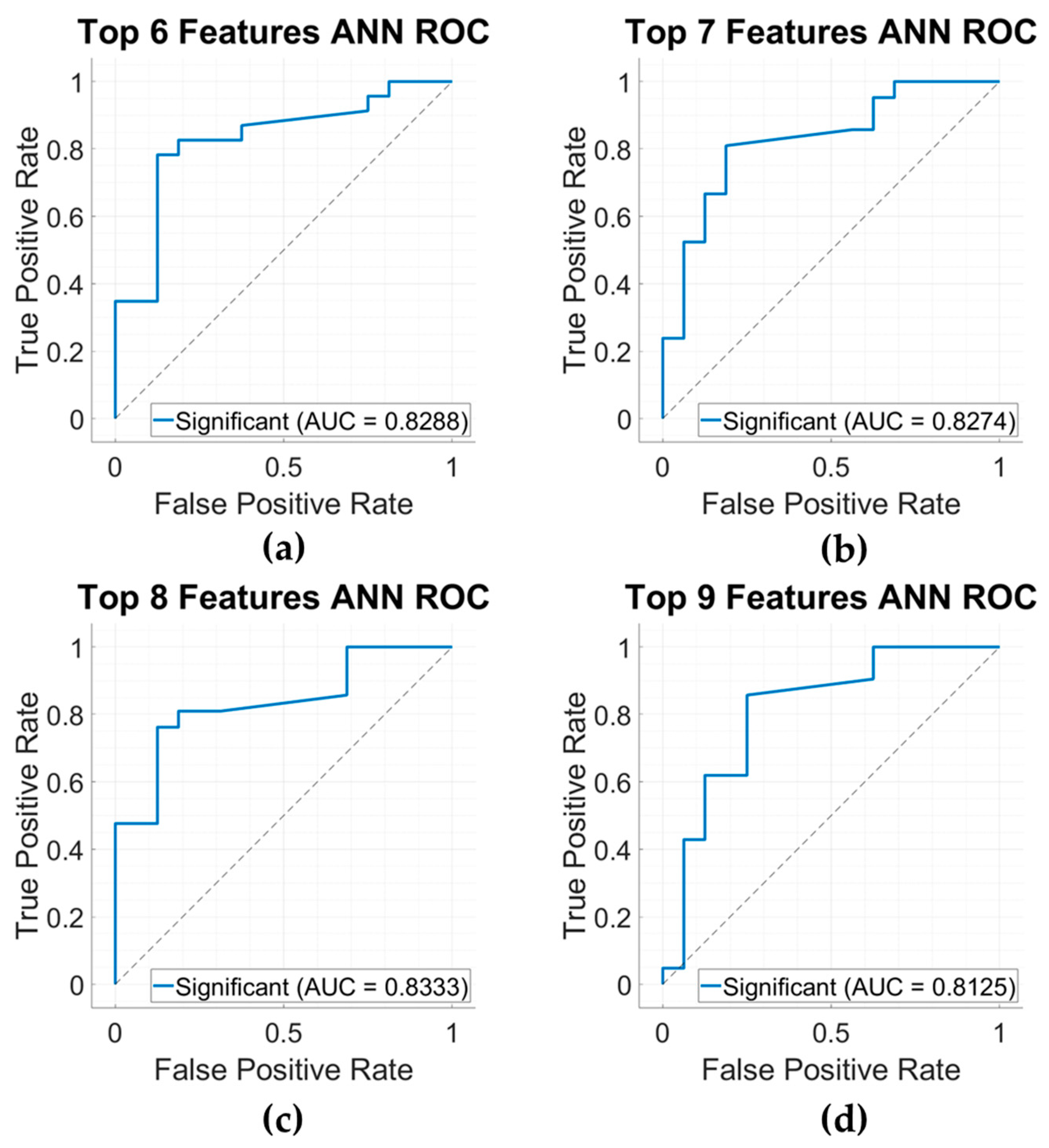
Receiver operator characteristic (ROC) curves were also generated, and the area under the curve (AUC) was calculated as an additional measure to determine suitability for the models. An ROC AUC of greater than 0.7 was considered acceptable and values greater than 0.8 were considered good. A value near 0.5 was considered similar to a coin-flip classifier [47].

3. Results

3.1. Dataset Summary

A total of 19 studies encompassing 132 experiments were included in the dataset. A summary of the sources is provided in Table 2. Approximately 60% of experiments in the dataset were considered successful by the source.

3.2. FEM Simulation of Monopolar Electrode

The results of the COMSOL simulation are shown below in Figure 1 during the 90 V, 100 ms pulses from [45]. These results showcase the high variability in electric field strengths in tissues, even when uniform voltages are applied. The electrical parameters used in the simulated muscle were taken from [16].

3.3. χ 2 Results for Feature Selection

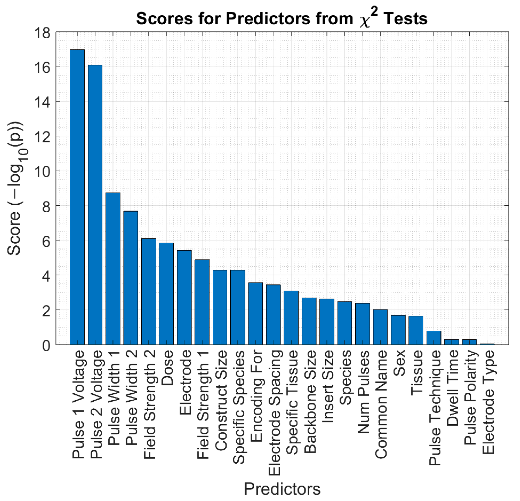
The results of the χ 2 test are provided in Figure 2. The highest-ranked features were pulse voltage and pulse width, which means that these variables were most highly correlated with the outcome variable, either the ‘success’ or ‘failure’ of the treatment. Scores are given as −log(p), where p is the p-value of the corresponding χ 2 test between the individual feature and the outcome of the experiments. Scores greater than 1 were considered to significantly contribute to the prediction of the outcome variable [57]. The differences between subsequent scores decreased after the highest four scores, so those scores were always included as part of the limited predictor dataset.
The bootstrapped rankings of 100 resamplings are shown in Figure 3. While several predictors changed relative ranks compared to the single-sample χ 2 testing described in Figure 2, the top four predictors remained the same, making them robust to the resampling of the data.

3.4. Model Results

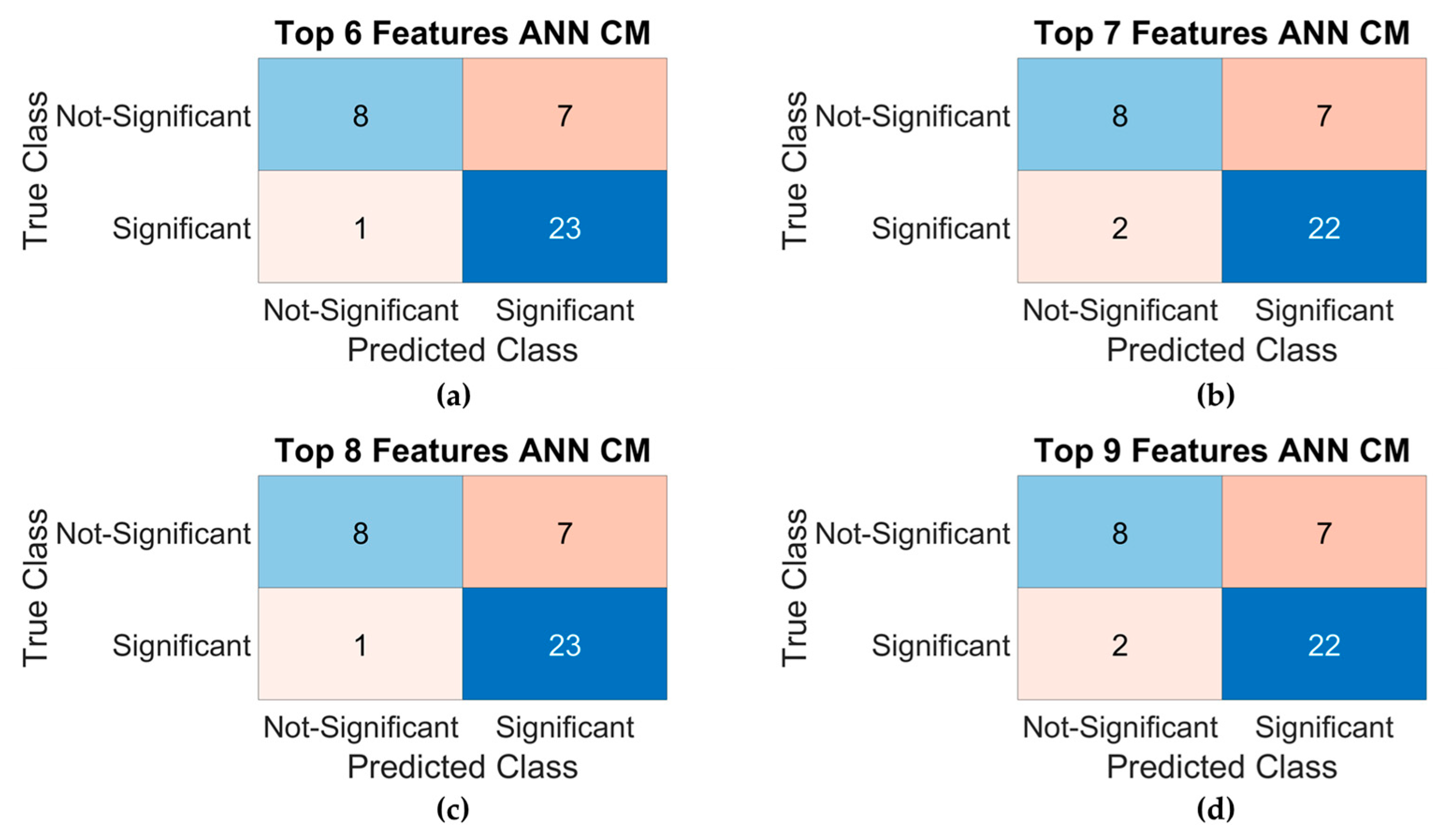
All models generated performed similarly in terms of accuracy, with feature-limited models outperforming their basic and parameter-optimized variants and accuracies ranging from 53% to 72%. Model performance began to differentiate when looking at the more specific figures of merit. The sensitivity and F1-scores of the Basic ANN, λ -Optimized ANN, and Basic SVM were particularly poor in performance, and the MCC of the Basic ANN suggested that it was only marginally better than a coin flip. Table 3 summarizes the figures of merit for all models. Figure 4 provides the CMs and Figure 5 provides the ROC curves for the top four ANN models by ROC AUC: 6–9 top feature ANNs. All performance metrics were calculated with the original test set, without re-randomizing the data, thereby avoiding possible inflated performance by including a subset of training data.
While the basic SVM outperformed the basic ANN, restricting features fed into the ANN resulted in a marked jump in performance in comparison with even the basic SVM. Also of note is that all models had drastically different results for specificity and sensitivity, with specificity being markedly higher in all cases, regardless of overall performance. The similar results for the top 6–9 ANN models also reaffirmed that adding further features past the top 6 based on the χ 2 results in Section 3.3 did not improve model performance.

4. Discussion

To date, GET optimization requires the extensive use of costly cell cultures and animals to refine ideal PEF conditions and associated parameters to maximize expression with minimal side effects. A typical new GET study will iterate on the variables presented in Table 2 to achieve a set of working conditions that achieve the desired outcome. These myriad parameters are typically informed only by lab history itself, with highly varied preferences between labs. A model that is informed by a large body of data from multiple labs has the potential to enable physical studies to start from a more advantageous state and reduce the need for costly materials and lab time. These models narrow down the need for parameters that need to be tested empirically in animals for specific tissues with specific electrode configurations. Ultimately, this would reduce the time to clinical translation and get these new parameters into the hands of practicing clinicians sooner. This work presents a first foray into developing such ML algorithms to inform GET working conditions to reduce the variability, cost, and complexity of studies and improve overall study results with higher fidelity GET optimization informed by a trained predictive model.
As a first step, basic ANN and SVM models were trained on the dataset without any feature reduction, with the results presented in Table 3. While the SVM model performed better than the ANN model, both models performed poorly. The accuracies, sensitivities, and specificities for both models were all below 70% and the MCCs for both models were about or below the value expected for a coin-flip predictor. The Basic SVM model did have an ‘acceptable’ AUC of >0.8, but, given the poor performance in other metrics, this metric on its own was not considered acceptable.
In the training of ANNs, there are a multitude of parameters to adjust that may increase the performance of the underlying model. The first of these is the regularization strength, λ . This parameter can be adjusted by iterating the underlying model under different values of λ and choosing the model that reduces error during validation. The optimized model had better performance than the Basic ANN, as shown in Table 3, but still performed relatively poorly when compared to desired thresholds. These were not unexpected results, as most machine learning models require large datasets to begin to achieve higher levels of accuracy and performance. ANNs specifically scale the required dataset size based on the number of features used to describe each data point. So, the more variables that are used to describe the underlying data, the more data points are required for an ANN to approach usable metrics.
To reduce the effect of the relatively small sample size, the number of features used to train the models was reduced using the results of a bootstrapped χ 2 test. The results of one iteration of this test are provided in Figure 2, which shows that voltage and pulse width were amongst the features that most strongly predicted the outcome. This outcome follows prevailing theories in the field, where labs will generally start by adjusting physical pulse parameters when attempting to optimize a procedure. However, due to variability in the data, a bootstrapped version of the test was completed, where the data were resampled 100 times and 95% confidence intervals were plotted for each of the ranks. These data are summarized in Figure 3. Even after bootstrapping, these results show that, in the available data, pulse and electrode design were the most impactful features when it came to successful outcomes, reinforcing the explainability of the underlying ‘logic’ of the machine learning models.
Using the results of the χ 2 analysis, reduced-feature-set datasets were constructed using the top 5, 6, 7, 8, and 9 features. The minimum feature set of five was determined as the threshold in the χ 2 results where the subsequent features did not have a large difference in rank score from the previous features in Figure 2. These reduced-feature datasets were used to train ANNs and SVMs, with the resulting metrics tabulated in Table 3. As expected, the models trained on reduced features had higher performance than the full-feature datasets. Four out of five models had an AUC > 0.8 and three of the five also had improved MCCs > 0.3. The ROC curves and truth tables of these selected models are provided in Figure 4, with their performance metrics presented in Table 3 alongside those of the other models.
The SVM versions of the reduced-feature models did not see such a boost in performance as observed with the ANN models. In most cases, the performance was reduced compared to the full-feature model. This result was likely due to the reduced features the SVM had available to train the model. While ANNs act as if they have a ‘logic’ to their decisions, SVMs create support vectors from the available training data to separate the outcomes in a higher dimensional space. Reducing the feature size reduces the available variables for the SVM to create these support vectors, which is likely why the reduced-feature SVM models lost performance compared to the ANN models.
Ultimately, the goal of these models is to inform researchers and clinicians of the potential of a proposed set of parameters before spending resources to investigate them directly. However, as shown in the collected dataset, the field at large operates on a wide range of species and tissue types and uses a variety of plasmid DNA, depending on the application. The wide variability in application and subject tissue presents a limitation in model generalizability. While these models would perform well given the tissues, species, or electrodes that the models were trained on, the introduction of a tissue or electrode unknown to the model would likely not provide similar results to those presented here. A solution to this generalization problem is to expand the electrode, tissue, and species variables beyond a simple label. FEM simulations of electric field strengths between the electrodes would alleviate part of this unknown by allowing for the entry of electrode and tissue parameters directly into both the FEM and machine learning models, effectively specifying electrodes by their field distributions and tissues by their electrical parameters rather than by labels. This one step would eliminate a large portion of the limitation in the generalizability of these models, but would take a concerted effort by the community at large to achieve.
Finally, globally, there is a notable limitation of this study due to inherent variabilities from lab to lab and even from operators within labs in how experiments are designed and carried out, how data are reported, and how field strengths are determined. The variability of GET test equipment and the sensitivity of the analyses are inherent in such an analysis as there is a lack of standardization in the hardware, software, test methods, and reporting, as we noted in reviewing 19 different papers for this model. Field strengths in particular are often reported in a simplified manner using Equation (1). This can be an oversimplification, as shown in Figure 1, where the field strengths and thus voltage distributions are anything but uniform. Furthermore, it is not typical for labs to report failed experiments unless they are relevant in the context of reporting successful treatment, such as in the case of a known negative control. This leads to lopsided datasets that are full of successes, with very few failures. Even though this dataset ended up with a 60–40% split of successes vs. failures, the majority of the ‘failures’ were, in fact, control data that were known to produce either an insignificant effect or no effect whatsoever. This leads to a false uniformity in the conditions leading to the failure of treatment and resulting disparities between sensitivity and specificity metrics. Publishing, or at least sharing, unsuccessful testing results will not only provide additional data points to train these models on but also add variability to unsuccessful conditions, which is not present in the current literature.
In creating a robust model, all data should be considered, regardless of the success or failure of the attempted treatment. Furthermore, efforts to standardize and monitor the pulsing, delivered PEF, its conditions, and controlled and standardized analyses are crucial to training and an area of further research for our group. The optimal solution to standardization is for all experiments to come with accompanying FEM simulation data, captured pulse waveforms, and histology in the treatment area. These data could then be fed as images or multidimensional arrays into a machine learning model to more accurately inform the model of real spatial and temporal variations in field strength during treatment and correlate those variable field strengths to effective transfection in the underlying tissue. These data would also help alleviate lab-to-lab variability as, even if labs define treatment parameters differently, standardized values could be extracted from the provided data.

5. Conclusions

This work presented a first set of ML analyses from 132 data points gathered from 19 published papers to generate algorithms for optimizing GET conditions in silico. This initial training highlighted the importance of pulse voltage and pulse width (added values of successful pulse parameters), followed distantly by field strength, dose, and electrode configuration as guiding design principles for effective GET. The initial results show that it is possible to generate an ML model to inform optimal GET parameters to reduce the required time, cost, and animal numbers in future experiments. While the initial ANN models performed well, improvements will require the contribution of additional GET data including any unsuccessful treatments, as well as the more accurate modeling of real electrical parameters in the tissues and cells under study.

Author Contributions

Conceptualization, A.O., M.F. and A.B.; methodology, A.O.; software, A.O.; validation, A.O. and A.B.; formal analysis, A.O.; investigation, A.O.; data curation, A.O.; writing—original draft preparation, A.O.; writing—review and editing, A.O., M.F. and A.B.; visualization, A.O. and A.B.; project administration, A.B. and M.F. All authors have read and agreed to the published version of the manuscript.

Funding

This research received no external funding.

Institutional Review Board Statement

Not applicable.

Informed Consent Statement

Not applicable.

Data Availability Statement

The data analyzed in this study are available in the appropriately cited articles in the methods section. The model data supporting the conclusions of the article will be made available by the authors upon request.

Conflicts of Interest

The authors declare no conflicts of interest.

References

  1. Anguela, X.M.; High, K.A. Entering the modern era of gene therapy. Annu. Rev. Med. 2019, 70, 273–288. [Google Scholar] [CrossRef] [PubMed]
  2. Potter, H.; Heller, R. Transfection by electroporation. Curr. Protoc. Mol. Biol. 2018, 121, 9.3. 1–9.3. 13. [Google Scholar] [CrossRef] [PubMed]
  3. Nishi, T.; Yoshizato, K.; Yamashiro, S.; Takeshima, H.; Sato, K.; Hamada, K.; Kitamura, I.; Yoshimura, T.; Saya, H.; Kuratsu, J.-i. High-efficiency in vivo gene transfer using intraarterial plasmid DNA injection following in vivo electroporation. Cancer Res. 1996, 56, 1050–1055. [Google Scholar] [PubMed]
  4. Jaroszeski, M.J.; Gilbert, R.; Nicolau, C.; Heller, R. In vivo gene delivery by electroporation. Adv. Drug Deliv. Rev. 1999, 35, 131–137. [Google Scholar] [CrossRef]
  5. Boye, C.; Arpag, S.; Francis, M.; DeClemente, S.; West, A.; Heller, R.; Bulysheva, A. Reduction of plasmid vector backbone length enhances reporter gene expression. Bioelectrochemistry 2022, 144, 107981. [Google Scholar] [CrossRef]
  6. Miklavcic, D.; Semrov, D.; Mekid, H.; Mir, L. In vivo electroporation threshold determination. In Proceedings of the 22nd Annual International Conference of the IEEE Engineering in Medicine and Biology Society (cat. No. 00CH37143), Chicago, IL, USA, 23–28 July 2000; pp. 2815–2818. [Google Scholar]
  7. Meglič, S.H.; Pavlin, M. The impact of impaired DNA mobility on gene electrotransfer efficiency: Analysis in 3D model. BioMed. Eng. OnLine 2021, 20, 85. [Google Scholar] [CrossRef]
  8. Zhang, H.; Ji, X.; Zang, L.; Yan, S.; Wu, X. Process Analysis and Parameter Selection of Cardiomyocyte Electroporation Based on the Finite Element Method. Cardiovasc. Eng. Technol. 2024, 15, 22–38. [Google Scholar] [CrossRef] [PubMed]
  9. Zhou, C.; Yan, Z.; Liu, K. Response characteristics and optimization of electroporation: Simulation based on finite element method. Electromagn. Biol. Med. 2021, 40, 321–337. [Google Scholar] [CrossRef]
  10. Langus, J.; Kranjc, M.; Kos, B.; Šuštar, T.; Miklavčič, D. Dynamic finite-element model for efficient modelling of electric currents in electroporated tissue. Sci. Rep. 2016, 6, 26409. [Google Scholar] [CrossRef]
  11. Ferreira, E.; Potier, E.; Logeart-Avramoglou, D.; Salomskaite-Davalgiene, S.; Mir, L.M.; Petite, H. Optimization of a gene electrotransfer method for mesenchymal stem cell transfection. Gene Ther. 2008, 15, 537–544. [Google Scholar] [CrossRef]
  12. Heller, R.; Lundberg, C.M.; Burcus, N.; Edelblute, C.; Guo, S. Gene electrotransfer of plasmids encoding cytokines as an effective immunotherapy approach for melanoma. J. Immunol. 2016, 196, 213.16. [Google Scholar] [CrossRef]
  13. Peng, W.; Polajžer, T.; Yao, C.; Miklavčič, D. Dynamics of cell death due to electroporation using different pulse parameters as revealed by different viability assays. Ann. Biomed. Eng. 2024, 52, 22–35. [Google Scholar] [CrossRef] [PubMed]
  14. Saulis, G.; Saulė, R. Comparison of electroporation threshold for different cell lines in vitro. Acta Phys. Pol. A 2009, 115, 1056–1058. [Google Scholar] [CrossRef]
  15. Forjanič, T.; Markelc, B.; Marčan, M.; Bellard, E.; Couillaud, F.; Golzio, M.; Miklavčič, D. Electroporation-induced stress response and its effect on gene electrotransfer efficacy: In vivo imaging and numerical modeling. IEEE Trans. Biomed. Eng. 2019, 66, 2671–2683. [Google Scholar] [CrossRef] [PubMed]
  16. Gabriel, S.; Lau, R.; Gabriel, C. The dielectric properties of biological tissues: III. Parametric models for the dielectric spectrum of tissues. Phys. Med. Biol. 1996, 41, 2271. [Google Scholar] [CrossRef]
  17. Davalos, R.V.; Rubinsky, B.; Otten, D.M. A feasibility study for electrical impedance tomography as a means to monitor tissue electroporation for molecular medicine. IEEE Trans. Biomed. Eng. 2002, 49, 400–403. [Google Scholar] [CrossRef]
  18. Davalos, R.V.; Otten, D.M.; Mir, L.M.; Rubinsky, B. Electrical impedance tomography for imaging tissue electroporation. IEEE Trans. Biomed. Eng. 2004, 51, 761–767. [Google Scholar] [CrossRef]
  19. Ivorra, A.; Rubinsky, B. In vivo electrical impedance measurements during and after electroporation of rat liver. Bioelectrochemistry 2007, 70, 287–295. [Google Scholar] [CrossRef]
  20. Atkins, R.M.; Fawcett, T.J.; Gilbert, R.; Hoff, A.M.; Connolly, R.; Brown, D.W.; Llewellyn, A.J.; Jaroszeski, M.J. Impedance spectroscopy as an indicator for successful in vivo electric field mediated gene delivery in a murine model. Bioelectrochemistry 2017, 115, 33–40. [Google Scholar] [CrossRef]
  21. Moisescu, M.G.; Radu, M.; Kovacs, E.; Mir, L.M.; Savopol, T. Changes of cell electrical parameters induced by electroporation. A dielectrophoresis study. Biochim. Et Biophys. Acta (BBA)-Biomembr. 2013, 1828, 365–372. [Google Scholar] [CrossRef]
  22. Daud, A.I.; DeConti, R.C.; Andrews, S.; Urbas, P.; Riker, A.I.; Sondak, V.K.; Munster, P.N.; Sullivan, D.M.; Ugen, K.E.; Messina, J.L. Phase I trial of interleukin-12 plasmid electroporation in patients with metastatic melanoma. J. Clin. Oncol. 2008, 26, 5896–5903. [Google Scholar] [CrossRef] [PubMed]
  23. Daud, A.; Algazi, A.P.; Ashworth, M.T.; Fong, L.; Lewis, J.; Chan, S.E.; Buljan, M.; Molina, M.A.; Takamura, K.T.; Diep, T.T. Systemic antitumor effect and clinical response in a phase 2 trial of intratumoral electroporation of plasmid interleukin-12 in patients with advanced melanoma. J. Clin. Oncol. 2014, 32, 15. [Google Scholar] [CrossRef]
  24. Lucas, M.L.; Jaroszeski, M.J.; Gilbert, R.; Heller, R. In vivo electroporation using an exponentially enhanced pulse: A new waveform. DNA Cell Biol. 2001, 20, 183–188. [Google Scholar] [CrossRef] [PubMed]
  25. Pavšelj, N.; Préat, V. DNA electrotransfer into the skin using a combination of one high-and one low-voltage pulse. J. Control. Release 2005, 106, 407–415. [Google Scholar] [CrossRef] [PubMed]
  26. Guo, S.; Jackson, D.L.; Burcus, N.I.; Chen, Y.-J.; Xiao, S.; Heller, R. Gene electrotransfer enhanced by nanosecond pulsed electric fields. Mol. Ther.-Methods Clin. Dev. 2014, 1-8, 1–8. [Google Scholar] [CrossRef] [PubMed]
  27. Donate, A.; Bulysheva, A.; Edelblute, C.; Jung, D.; Malik, M.A.; Guo, S.; Burcus, N.; Schoenbach, K.; Heller, R. Thermal assisted in vivo gene electrotransfer. Curr. Gene Ther. 2016, 16, 83–89. [Google Scholar] [CrossRef]
  28. Bulysheva, A.; Hornef, J.; Edelblute, C.; Jiang, C.; Schoenbach, K.; Lundberg, C.; Malik, M.A.; Heller, R. Coalesced thermal and electrotransfer mediated delivery of plasmid DNA to the skin. Bioelectrochemistry 2019, 125, 127–133. [Google Scholar] [CrossRef]
  29. López-Alonso, B.; Sarnago, H.; Lucía, Ó.; Briz, P.; Burdío, J.M. Real-time impedance monitoring during electroporation processes in vegetal tissue using a high-performance generator. Sensors 2020, 20, 3158. [Google Scholar] [CrossRef]
  30. Atkins, R.M.; Fawcett, T.J.; Gilbert, R.; Hoff, A.M.; Connolly, R.; Brown, D.W.; Jaroszeski, M.J. Real-time impedance feedback to enhance cutaneous gene electrotransfer in a murine skin model. Bioelectrochemistry 2021, 142, 107885. [Google Scholar] [CrossRef]
  31. Barnes, H.; Humphries, S.M.; George, P.M.; Assayag, D.; Glaspole, I.; Mackintosh, J.A.; Corte, T.J.; Glassberg, M.; Johannson, K.A.; Calandriello, L. Machine learning in radiology: The new frontier in interstitial lung diseases. Lancet Digit. Health 2023, 5, e41–e50. [Google Scholar] [CrossRef]
  32. Kumar, A.; Singh, S.K.; Saxena, S.; Lakshmanan, K.; Sangaiah, A.K.; Chauhan, H.; Shrivastava, S.; Singh, R.K. Deep feature learning for histopathological image classification of canine mammary tumors and human breast cancer. Inf. Sci. 2020, 508, 405–421. [Google Scholar] [CrossRef]
  33. Huttunen, R.; Leppänen, T.; Duce, B.; Arnardottir, E.S.; Nikkonen, S.; Myllymaa, S.; Töyräs, J.; Korkalainen, H. A Comparison of Signal Combinations for Deep Learning-Based Simultaneous Sleep Staging and Respiratory Event Detection. IEEE Trans. Biomed. Eng. 2022, 70, 1704–1714. [Google Scholar] [CrossRef] [PubMed]
  34. Zappatore, M.; Cerfeda, G.; Merla, C.; Tarricone, L. Machine learning for H-FIRE protocols: Tuning parameters for high-frequency irreversible electroporation by machine learning. IEEE Microw. Mag. 2021, 22, 42–59. [Google Scholar] [CrossRef]
  35. De Cillis, A.; Merla, C.; Tarricone, L.; Zappatore, M. Machine-Learning for Optimization of Electrodes and Waveforms for Electroporation. In Proceedings of the 2022 International Conference on Electromagnetics in Advanced Applications (ICEAA), Cape Town, South Africa, 5–9 September 2022; pp. 031–034. [Google Scholar]
  36. Eresen, A.; Zhou, K.; Sun, C.; Shangguan, J.; Wang, B.; Pan, L.; Hu, S.; Pang, Y.; Zhang, Z.; Tran, R.M.N. Early assessment of irreversible electroporation ablation outcomes by analyzing MRI texture: Preclinical study in an animal model of liver tumor. Am. J. Transl. Res. 2022, 14, 5541. [Google Scholar]
  37. Briz, P.; López-Alonso, B.; Sarnago, H.; Burdío, J.; Lucía, O. Tumor location on electroporation therapies by means of multi-electrode structures and machine learning. Bioelectrochemistry 2023, 154, 108510. [Google Scholar] [CrossRef]
  38. Patino, C.A.; Mukherjee, P.; Lemaitre, V.; Pathak, N.; Espinosa, H.D. Deep learning and computer vision strategies for automated gene editing with a single-cell electroporation platform. SLAS Technol. Transl. Life Sci. Innov. 2021, 26, 26–36. [Google Scholar] [CrossRef]
  39. Vitale, J.; Sassi, M.; Pecchia, L. A Machine Learning Approach for Predicting Electrophysiological Responses in Genetically Modified HEK Cells. In Proceedings of the European Medical and Biological Engineering Conference, Portoroz, Slovenia, 9–13 June 2024; pp. 1–14. [Google Scholar]
  40. Duda, R.O.; Hart, P.E. Pattern Classification and Scene Analysis; Wiley: New York, NY, USA, 1973; Volume 3. [Google Scholar]
  41. Bishop, C.M.; Nasrabadi, N.M. Pattern Recognition and Machine Learning; Springer: Berlin/Heidelberg, Germany, 2006; Volume 4. [Google Scholar]
  42. Heller, R.; Jaroszeski, M.; Atkin, A.; Moradpour, D.; Gilbert, R.; Wands, J.; Nicolau, C. In vivo gene electroinjection and expression in rat liver. FEBS Lett. 1996, 389, 225–228. [Google Scholar] [CrossRef] [PubMed]
  43. Heller, L.; Jaroszeski, M.; Coppola, D.; Pottinger, C.; Gilbert, R.; Heller, R. Electrically mediated plasmid DNA delivery to hepatocellular carcinomas in vivo. Gene Ther. 2000, 7, 826–829. [Google Scholar] [CrossRef]
  44. Pasquet, L.; Chabot, S.; Bellard, E.; Markelc, B.; Rols, M.-P.; Reynes, J.-P.; Tiraby, G.; Couillaud, F.; Teissie, J.; Golzio, M. Safe and efficient novel approach for non-invasive gene electrotransfer to skin. Sci. Rep. 2018, 8, 16833. [Google Scholar] [CrossRef]
  45. Boye, C.; Arpag, S.; Burcus, N.; Lundberg, C.; DeClemente, S.; Heller, R.; Francis, M.; Bulysheva, A. Cardioporation enhances myocardial gene expression in rat heart. Bioelectrochemistry 2021, 142, 107892. [Google Scholar] [CrossRef]
  46. Chicco, D.; Jurman, G. The advantages of the Matthews correlation coefficient (MCC) over F1 score and accuracy in binary classification evaluation. BMC Genom. 2020, 21, 6. [Google Scholar] [CrossRef] [PubMed]
  47. Mandrekar, J.N. Receiver operating characteristic curve in diagnostic test assessment. J. Thorac. Oncol. 2010, 5, 1315–1316. [Google Scholar] [CrossRef] [PubMed]
  48. Rols, M.-P.; Delteil, C.; Golzio, M.; Dumond, P.; Cros, S.; Teissie, J. In vivo electrically mediated protein and gene transfer in murine melanoma. Nat. Biotechnol. 1998, 16, 168–171. [Google Scholar] [CrossRef] [PubMed]
  49. Heller, L.; Pottinger, C.; Jaroszeski, M.J.; Gilbert, R.; Heller, R. In vivo electroporation of plasmids encoding GM-CSF or interleukin-2 into existing B16 melanomas combined with electrochemotherapy induces long-term antitumour immunity. Melanoma Res. 2000, 10, 577–583. [Google Scholar] [CrossRef] [PubMed]
  50. Zhang, L.; Nolan, E.; Kreitschitz, S.; Rabussay, D.P. Enhanced delivery of naked DNA to the skin by non-invasive in vivo electroporation. Biochim. Et Biophys. Acta (BBA)-Gen. Subj. 2002, 1572, 1–9. [Google Scholar] [CrossRef]
  51. Ferraro, B.; Cruz, Y.L.; Coppola, D.; Heller, R. Intradermal delivery of plasmid VEGF165 by electroporation promotes wound healing. Mol. Ther. 2009, 17, 651–657. [Google Scholar] [CrossRef]
  52. Heller, R.; Cruz, Y.; Heller, L.C.; Gilbert, R.A.; Jaroszeski, M.J. Electrically mediated delivery of plasmid DNA to the skin, using a multielectrode array. Hum. Gene Ther. 2010, 21, 357–362. [Google Scholar] [CrossRef]
  53. Reberšek, M.; Faurie, C.; Kandušer, M.; Čorović, S.; Teissié, J.; Rols, M.-P.; Miklavčič, D. Electroporator with automatic change of electric field direction improves gene electrotransfer in-vitro. Biomed. Eng. Online 2007, 6, 25. [Google Scholar] [CrossRef]
  54. Hojman, P.; Zibert, J.R.; Gissel, H.; Eriksen, J.; Gehl, J. Gene expression profiles in skeletal muscle after gene electrotransfer. BMC Mol. Biol. 2007, 8, 56. [Google Scholar] [CrossRef]
  55. Kos, S.; Vanvarenberg, K.; Dolinsek, T.; Cemazar, M.; Jelenc, J.; Préat, V.; Sersa, G.; Vandermeulen, G. Gene electrotransfer into skin using noninvasive multi-electrode array for vaccination and wound healing. Bioelectrochemistry 2017, 114, 33–41. [Google Scholar] [CrossRef]
  56. Bulysheva, A.A.; Hargrave, B.; Burcus, N.; Lundberg, C.G.; Murray, L.; Heller, R. Vascular endothelial growth factor-A gene electrotransfer promotes angiogenesis in a porcine model of cardiac ischemia. Gene Ther. 2016, 23, 649–656. [Google Scholar] [CrossRef] [PubMed]
  57. Greenwood, P.E.; Nikulin, M.S. A Guide to Chi-Squared Testing; John Wiley & Sons: Hoboken, NJ, USA, 1996; Volume 280. [Google Scholar]
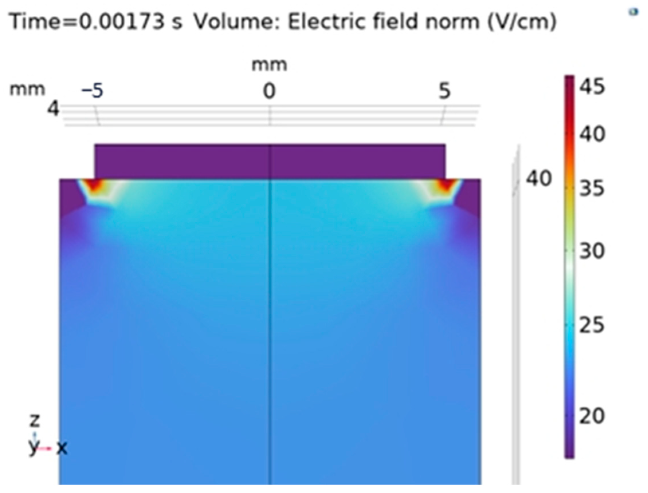
Figure 1. Magnitude of the electric field ( E ) in cardiac muscle directly below the 1 cm2 platinum electrode during 100 ms pulse of 90 V. Max field is fringe field at 45 V/cm with bulk field at 25 V/cm.
Applsci 14 11601 g001
Figure 2. Pulse voltage and width were variables most highly correlated with the outcome variable. Scores from χ 2 testing between individual features and significance variable. Scores are ranked from high (left) to low (right) in order of relation to the true outcomes of each experiment. This figure is the result of one set of χ 2 tests.
Applsci 14 11601 g002
Figure 3. After 100 resamplings, pulse voltage and pulse width remained highly ranked features. The bars represent 95% confidence intervals for the mean (). A rank of 1 corresponds to the best predictor, whereas a rank of 24 corresponds to the worst predictor.
Applsci 14 11601 g003
Figure 4. Confusion matrices for the top four ANN models showed similar performance in terms of true positive and true negative rates in 39 validation cases when only using the (a) top 6 features, (b) top 7 features, (c) top 8 features, and (d) top 9 features.
Applsci 14 11601 g004
Figure 5. ROC AUC values and curves for each of the top 4 ANN models showed similarly acceptable values when the ANN was allowed access to only the (a) top 6 features, (b) top 7 features, (c) top 8 features, and (d) top 9 features.
Applsci 14 11601 g005
Table 1. Table of features from each of the source papers and their descriptions.
FeatureDescription
Common NameCommon name of plasmid used in study
DoseDose of plasmid in μg
ElectrodeElectrode configuration
Electrode TypePenetrating or non-penetrating electrode
Backbone NameName of backbone in plasmid
Promoter NameName of promoter in plasmid
Construct SizeSize of entire plasmid in kb
Backbone SizeSize of backbone of plasmid in kb
Insert SizeSize of insert of plasmid in kb
Encoding ForName of protein encoded for
Pulse TechniqueStraight pulsing between 2 electrodes or multielectrode array pulsing
Pulse PolaritySame or alternating polarity when different pulse parameters are used
Pulse V1/V2Pulse amplitude of the first/second pulse in volts
Field Strength 1/2Field strength of the first/second pulse in volts/cm
Pulse Width 1/2Pulse width of the first/second pulse in μs
Number of PulsesNumber of pulses/pulse trains
Dwell TimeTime between pulses/pulse trains in s
Electrode SpacingDistance between electrodes in cm
General/Specific TissueTarget tissue for the study
SexSex of the animal/source cells
General/Specific SpeciesSpecies of the animal/source cells
Expression LocationLocation(s) of expression determined via histology of the target tissue(s)
OutcomeSuccess or failure of the treatment based on source author(s) significance criteria
Table 2. Source papers with selection of features from each group of experiments showcasing the variability in existing GET studies.
SourcePlasmid Common NameSpecies/Cell LineElectrodePulse PolarityExperiments
[42]pRc/CMV-LucSprague Dawley Rat6-Needle CirclePositive7
[48]pUT531B6D2F1 Mouse2-PlatePositive10
[43] pCMV-Luc+Sprague Dawley Rat7-NeedlePositive11
[49]pCMV-Luc+BC57B1/6 Mouse7-NeedlePositive1
[49]pCMV-Luc+BC57B1/6 Mouse7-NeedlePositive4
[50]pLucSKH1 MouseCaliperAlternating12
[25]pCMVLucWistar RatCaliperPositive7
[51]pVEGFSprague Dawley Rat4-PlatePositive2
[52]gWiz-LucC57B1/6 MouseCaliper + 6-NeedlePositive8
[22]pUMVC3-hIL-12-NGVL3Human6-Needle CirclePositive24
[53]pEGFP-C1Chinese Hamster Ovarian Cells4-Pin CirclePositive + Alternating4
[54]phGFP-S655TC57Black/C Mouse2-PlateAlternating1
[54]phGFP-S655TWistar Rat2-PlateAlternating1
[26]gWiz-LucHaCaT CellsCuvettePositive2
[44]pCMV-tdTomatoC57Bl/6 MouseContact WirePositive9
[11]pDRIVE2-CMVMesenchymal Stem CellsCuvettePositive7
[55]pVAX2-LUCC57BL/6 MousePlate + 7-Pin HexPositive3
[56]pVax1-hVEGF165(pVEGF-A)Yorkshire Pig4-PinPositive1
[3]pCH110Wistar Rat2-PinPositive4
[45]gWiz-Luc and NTC9385R-LucSprague Dawley RatMonopolar + 4-PinPositive + Alternating4
[5]gWiz-Luc and NTC9385R-LucSprague Dawley RatCaliperAlternating10
Table 3. Figures of merit for each of the 14 machine learning models generated.
ModelAccuracySensitivitySpecificityF1-ScoreMCCROC AUC
Basic ANN59.0%0%100.0%0.0−1.00.6036
λ Optimized ANN66.7%56.3%73.9%0.58060.30500.6536
Hyperparameter Optimized ANN59.0%43.8%69.6%0.46670.13650.4875
Top 5 Features ANN71.8%43.8%91.3%0.56000.40920.4679
Top 6 Features ANN64.1%25.0%91.3%0.36360.22230.8478
Top 7 Features ANN69.2%43.8%87.0%0.53850.34590.8288
Top 8 Features ANN66.7%31.3%91.3%0.43480.28910.8274
Top 9 Features ANN69.2%37.5%91.3%0.50000.35090.8333
Basic SVM53.9%31.3%69.6%0.35710.00870.8125
Top 5 Features SVM59.0%0%100.0%0.0−1.00.4214
Top 6 Features SVM59.0%0%100.0%0.0−1.00.3234
Top 7 Features SVM64.1%31.3%87.0%0.41670.22180.6012
Top 8 Features SVM64.1%31.3%87.0%0.41670.22180.6012
Top 9 Features SVM64.1%31.3%87.0%0.41670.22180.5744
Disclaimer/Publisher’s Note: The statements, opinions and data contained in all publications are solely those of the individual author(s) and contributor(s) and not of MDPI and/or the editor(s). MDPI and/or the editor(s) disclaim responsibility for any injury to people or property resulting from any ideas, methods, instructions or products referred to in the content.