Improving Passband Characteristics in Chebyshev Sharpened Comb Decimation Filters

Featured Application

Decimation filters are important to eliminate aliasing in many areas, such as wireless communications, software-defined radio, oversampled analog–digital converters, instrumentation, hearing aids, etc. The comb filter is the simplest decimation filter. However, its aliasing rejection is low. Chebyshev sharpening of combs significantly increases the aliasing rejection. However, this process increases the passband droop, which may deteriorate the decimated signal. As a consequence, it is very important to compensate for the passband droop in the Chebyshev sharpened comb decimation filters.

Abstract

This work presents the design of optimal and multiplierless compensators for Chebyshev sharpened comb decimation filters. The narrowband and wideband compensators are proposed. For the narrowband, the compensator with a magnitude response is proposed in a sinusoidal form, while for the wideband, two compensators with magnitude responses of two sinusoidal functions are introduced. The optimum design is performed using particle swarm optimization (PSO), while the multiplierless design is realized by presenting optimum parameters in a signed-power-of-two (SPT) form. Unlike the methods in the literature, this approach presents flexibility in design, allowing for an exchange between the quality of optimization and the complexity. Comparisons with the compensators from the literature demonstrated that the proposed method provides much better compensation while requiring fewer or slightly increased number of adders. Possible practical applications and potential future research work are also included.

1. Introduction

The Kaiser–Hamming sharpening [1] of comb decimation filters was first introduced in [2] to improve the passband and stopband characteristics of the filters. Later, various improvements to the Kaiser sharpening method were presented [3,4,5,6,7]. The Chebyshev sharpening of comb decimation filters was first introduced by Coleman in [8]. This filter provides a high predetermined attenuation in all folding bands. However, the passband has a high passband droop. The author also proposed a pre-sharpening version in which the passband droop is decreased but still needs to be improved. The authors in [9] proposed a novel method based on interval analysis, while in [10,11], were proposed different Chebyshev sharpening polynomials and the optimal filters to compensate for the passband droop. The sharpening combs belong to the modified comb decimation filters. In [12], the method to design an optimal compensator for Chebyshev sharpening combs provides better compensation than the compensators in [11]. This work is based on particle swarm optimization (PSO) and sinusoidal magnitude response.

This paper is dedicated to the design of compensators for Chebyshev sharpened comb filters and extends the previous work [12]. The next section elaborates on compensators’ general importance and applications as well as their principal design methods, emphasizing their practicality and the potential real-world applications of the research. It then describes the detailed proposed design procedure, including the design steps and the corresponding MATLAB programs.

The novelty of this work includes the following:

• In addition to the Chebyshev comb decimators introduced in [10,11], the Coleman popular Chebyshev sharpened comb [8] is also inclusively included in our research.
• Three optimal and multipliers compensators are designed, all with sinusoidal magnitude responses, with different complexity for the Chebyshev sharpened comb filters [8,10,11].
• Unlike the methods in [10,11], normalization of the designed compensation filters is unnecessary.
• A generalized approach is provided since all designs are based on sinusoidal magnitude responses and optimizing the amplitudes of sinusoidal responses using PSO.
• The flexibility of the design is shown in choosing narrowband or wideband designs and a trade-off between the quality of compensation and the number of required adders.
• The design is simple since only one parameter in the narrowband case and two parameters in the wideband case should be optimized, unlike the approaches in the literature based on optimizing the compensator filter coefficients.

This paper is organized as described in the continuation. The next section introduces compensators, importance, applications and the narrowband and wideband designs. Section 3 presents in detail the passband compensation design of the Chebyshev sharpened combs introduced in [8,10,11]. Section 4 compares the methods from the literature and presents the impact of the proposed designs on the possible practical applications. It also provides some further ideas for potential future work.

2. Compensators: Applications and Design

2.1. What Is a Compensated Modified Comb Decimator, and Why Is It Important?

Compensators are a key area of research in the field of comb filters. A decimation comb compensator is a specialized digital signal processing (DSP) filter designed to combine decimation (reducing the sampling rate of a signal) with comb filtering, thereby improving the passband characteristics of comb filters [13,14,15,16] or modified comb filters [4,5,6,7,10,11,12,17] at a low sample rate, i.e., after the decimation.

Key components of a compensated modified comb decimator are as follows [18,19]:

Modified comb filter. The enhanced version of the comb filter acts as a simple digital filter to suppress aliasing and shape the spectrum before decimation. Typical modified-comb filters are Chebyshev sharpening comb filters.

Decimation. This process reduces the sampling rate by an integer factor.

Compensation. It refines the passband response of the modified comb filter.

The modified comb filter preprocesses the input signal, removing high-frequency components that might alias when the sampling rate is reduced. Aliasing, a common issue in signal processing, occurs when high-frequency components are incorrectly represented at a lower sampling rate, leading to distortion. The signal is then decimated by an integer factor M, called a decimation factor. The compensation stage minimizes any distortion introduced during filtering and decimation.

This combination provides an efficient method to transition from high-rate to low-rate signal domains while preserving essential information, making it invaluable in numerous real-world systems.

A compensated modified comb decimator is important for several reasons, particularly in modern communication systems and digital processing [18,19,20]:

• Efficient Sample Rate Reduction. The compensated modified comb decimator impressively reduces the sampling rate without introducing aliasing and distortion, thereby saving memory and processing resources. This efficiency is particularly valuable in high-speed analog-to-digital converter (ADC) systems.
• Low Complexity. The compensated modified comb decimators, with their simple structure involving addition and subtraction operations, offer reassurance in terms of computational efficiency. This simplicity makes them highly suitable for hardware implementation.
• Improved Signal Integrity. The compensated modified comb decimator plays a crucial role in ensuring improved signal integrity. By attenuating undesired spectral components and artifacts, they instill confidence in the fidelity of the decimated signal.
• Scalable Decimation. Compensated modified comb decimators can be cascaded for multi-stage decimation, reducing the complexity of handling large decimation factors.

Some typical applications of compensated modified comb decimators include digital communication [18,19,20,21,22,23], audio and video processing [24,25], software-defined radio (SDR) [26], data compression [27,28], biomedical signal processing [29,30], and test and measurement systems [31,32].

2.2. Design

Usually, comb compensators are designed as finite impulse response (FIR) filters using various optimization methods to ensure that the cascade of the comb and the compensator provides as low as possible deviation in the passband of interest. We will adopt the denotations, as shown in the continuation.

The comb filter of order K and the decimation factor M is denoted as follows:

$$H\left(z,K,M\right)={\left[{\displaystyle \frac{1-z^{-M}}{M(1-z^{-1})}}\right]}^K.$$

(1)

The Chebyshev sharpened comb is denoted as G(z) and the compensator as C(z).

Since the compensator works at a low rate, using the multirate identity [18,19], the compensated filter Gc(z), which is a cascade of the Chebyshev sharpened comb and compensator is given as follows:

Gc(z) = G(z)C(z^M).

(2)

As the comb compensators introduced in [13,14,15] have sinusoidal magnitude characteristics while exhibiting high-quality compensation, we propose using the sinusoidal magnitude responses for the compensators proposed in this work to ensure the generalized approach and simplicity of the design. We consider narrowband and wideband designs, as described below.

2.2.1. Narrowband Design

In this design, the passband frequency ω_p < π/4M. The magnitude characteristic is chosen as in [13],

$$C_1\left(e^{jM\omega }\right)=1+C_{11}{sin}^2\left({\displaystyle \frac{\omega M}{2}}\right),$$

(3)

where C₁₁ is the parameter of the design.

The system function of this filter is given as [13],

$$C_1\left(z\right)=2^{-2}\left[\left(-1+2z^{-1}-z^{-2}\right)C_{11}+2^2{z}^{-1}\right].$$

(4)

The compensator requires three adders and one multiplier. In a multiplierless design, the number of required adders equals:

$$N_1=3+N_{11},$$

(5)

where N₁₁ is the number of adders in the signed-power-of-two (SPT) form of C₁₁.

2.2.2. Wideband Design

In the wideband design the passband frequency ω_p equals π/4M ≤ ω_p ≤ π/2M. We consider two wideband sinusoidal compensators.

Extension of Narrowband Design

The magnitude response is given as [14]

$$C_2\left(e^{jM\omega }\right)=\left[1+C_{21}{sin}^2\left({\displaystyle \frac{\omega M}{2}}\right)\right]\times \left[1+C_{22}{sin}^4\left({\displaystyle \frac{\omega M}{2}}\right)\right],$$

(6)

where C₂₁ and C₂₂ are the parameters of the design.

The system function of this compensator is given as follows [14]:

$$\begin{gathered} C_2\left(z\right)=2^{-2}\left[\left(-1+2z^{-1}-z^{-2}\right)C_{21}+2^2{z}^{-1}\right]\times \\ \left[2^{-4}{C}_{22}\left[\left(1+z^{-4}-4(z^{-1}+z^{-3}\right)+{(2}^2+2)z^{-2}\right]+z^{-2}\right]. \end{gathered}$$

(7)

The compensator requires nine adders and two multipliers C₂₁ and C₂₂. The number of the required adders in a multiplierless design is given as

$$N_2=9+N_{21}+N_{22},$$

(8)

where N₂₁ and N₂₂ are the number of adders in SPT forms of C₂₁ and C₂₂, respectively.

To increase the flexibility of the design, we also consider the less complex compensator from [15] introduced in the next subsection.

Simplified Version of Compensator in [14]

The magnitude response is given as follows [15]:

$$C_3\left(e^{jM\omega }\right)=1+C_{31}{sin}^2\left({\displaystyle \frac{\omega M}{2}}\right)+C_{32}{sin}^4\left({\displaystyle \frac{\omega M}{2}}\right),$$

(9)

where C₃₁ and C₃₂ are parameters of the design.

The system function is given as [15],

$$C_2\left(z\right)=2^{-4}{C}_{32}\left(1-2z^{-2}\right)-\left(C_{31}+C_{32}\right)2^{-2}\left(z^{-1}-2z^{-2}+z^{-3}\right)+z^{-2}.$$

(10)

The compensator requires six adders, two multipliers, C₃₂, and the sum of C₃₂ and C₃₁. The number of the needed adders in a multiplierless design is

$${\mathrm{N}}_3=6+N_{32}+N_{312},$$

(11)

where N₃₂ and N₃₁₂ are the number of adders in SPT forms of C₃₂ and the sum of C₃₁ and C₃₂, respectively.

2.3. How to Obtain the Compensator Design Parameters?

We first consider optimum design to obtain the parameters in compensators (3), (6) and (9) in such a way that a minimum of the maximum passband deviation δ_o in the passband of interest, defined by the passband edge ω_p, equals

$$20\times {log}_{10}\left|G_c\left(e^{j\omega }\right)\right|\le {\delta }_{opt} \mathrm{for} 0\le \omega \le {\omega }_p,$$

(12)

where $G_c\left(e^{j\omega }\right)$ is given in (2), and the compensators are given in (3), (6) and (9).

The optimal design is obtained using particle swarm optimization (PSO) in MATLAB [33]. The multiplierless design is obtained by presenting the optimal parameters in a signed power-of-two (SPT) form.

The detailed design is described in the next section, while the MATLAB programs are explained in the Supplementary Material.

3. Passband Compensation of Chebyshev Sharpened Combs from [8,10,11]

We present the compensation of the Coleman Chebyshev comb [8] and Chebyshev combs in [10,11].

3.1. Steps of Design

In this section, we present the design steps.

STEP 1:

Choose the Chebyshev sharpened comb.

STEP 2:

Choose narrowband or wideband design, depending on the passband of interest.

In narrowband case, choose the filter C₁ in (3).

In the wideband case, choose between the filters C₂ given in (6) or the simplified version C₃, from (9).

STEP 3:

Find the optimal compensator parameters using PSO in MATLAB.

STEP 4:

Present the optimal compensator parameters in SPT forms using MATLAB, varying the number of adders.

STEP 5:

Compute the corresponding filter coefficients in the SPT form.

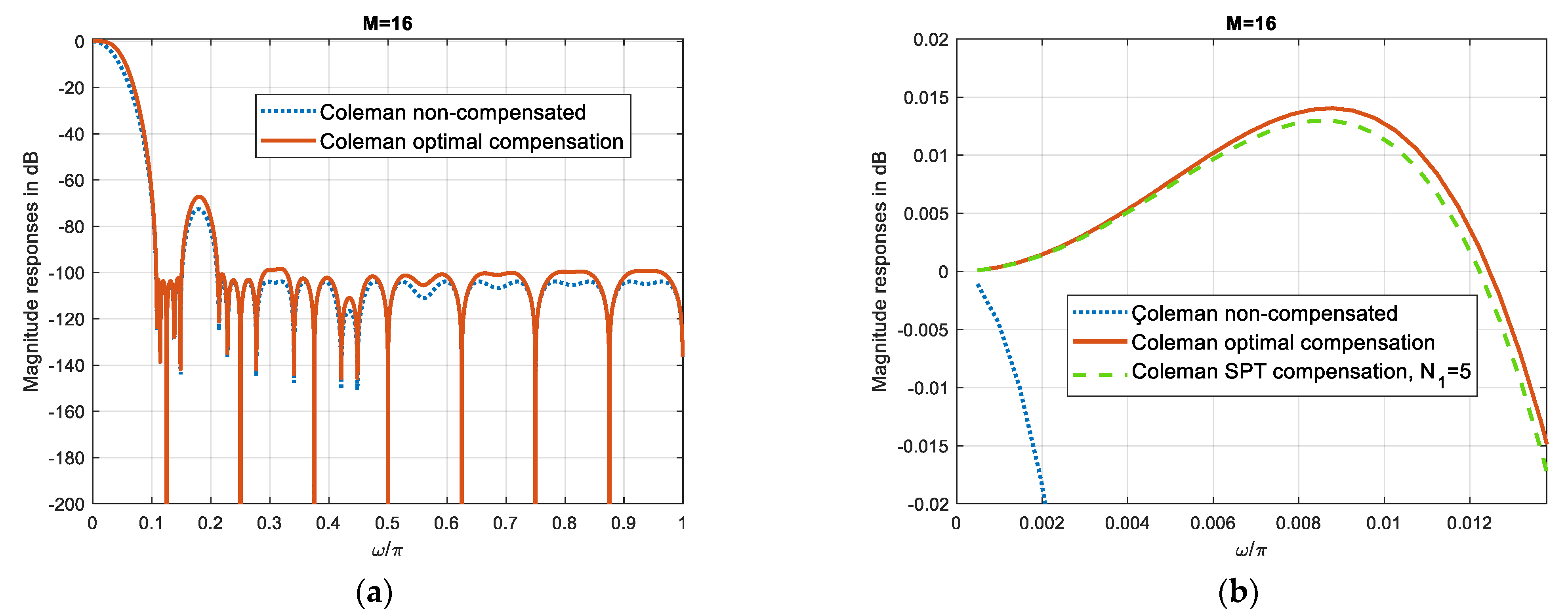
3.2. Coleman Chebyshev Sharpened Comb [8]

The fifth-order Chebyshev polynomial coefficients in [8] are [0, 5, −20, 16]. The decimation factor M = 16, and the attenuation in the stopbands is −100 dB [8].

3.2.1. Narrowband Compensation

We consider ω_p = 0.22π/M and the compensator C₁ in (3). Using PSO in MATLAB, we obtain C_11o = 0.9089 resulting in the optimum passband deviation of δ_o = 0.0141dB. Next, C_11o is presented in the SPT form varying the number of adders from four to seven, as shown in

Table 1. SPT compensator C₁ coefficients, passband deviation, and the number of adders.

C11	δ1 [dB]	N1
20-2−4	0.0274	4
20-2−3 + 2−5	0.0165	5
20-2−3 + 2−5 + 2−8	0.0145	6
20-2−3 + 2−5 + 2−8-2−10	0.0142	7

. It can be observed that we have approximately optimum compensation with seven adders, denoted in bold in Table 1.

Figure 1a compares overall magnitude responses of non-compensated Coleman filter and compensated with the optimum compensator (3). The compensation slightly deteriorates the stopband, as shown in Figure 1a. Figure 1b compares passbands of the Coleman non-compensated filter, compensated with the optimum filter and compensated with the SPT filter from Table 1 with N₁ = 5.

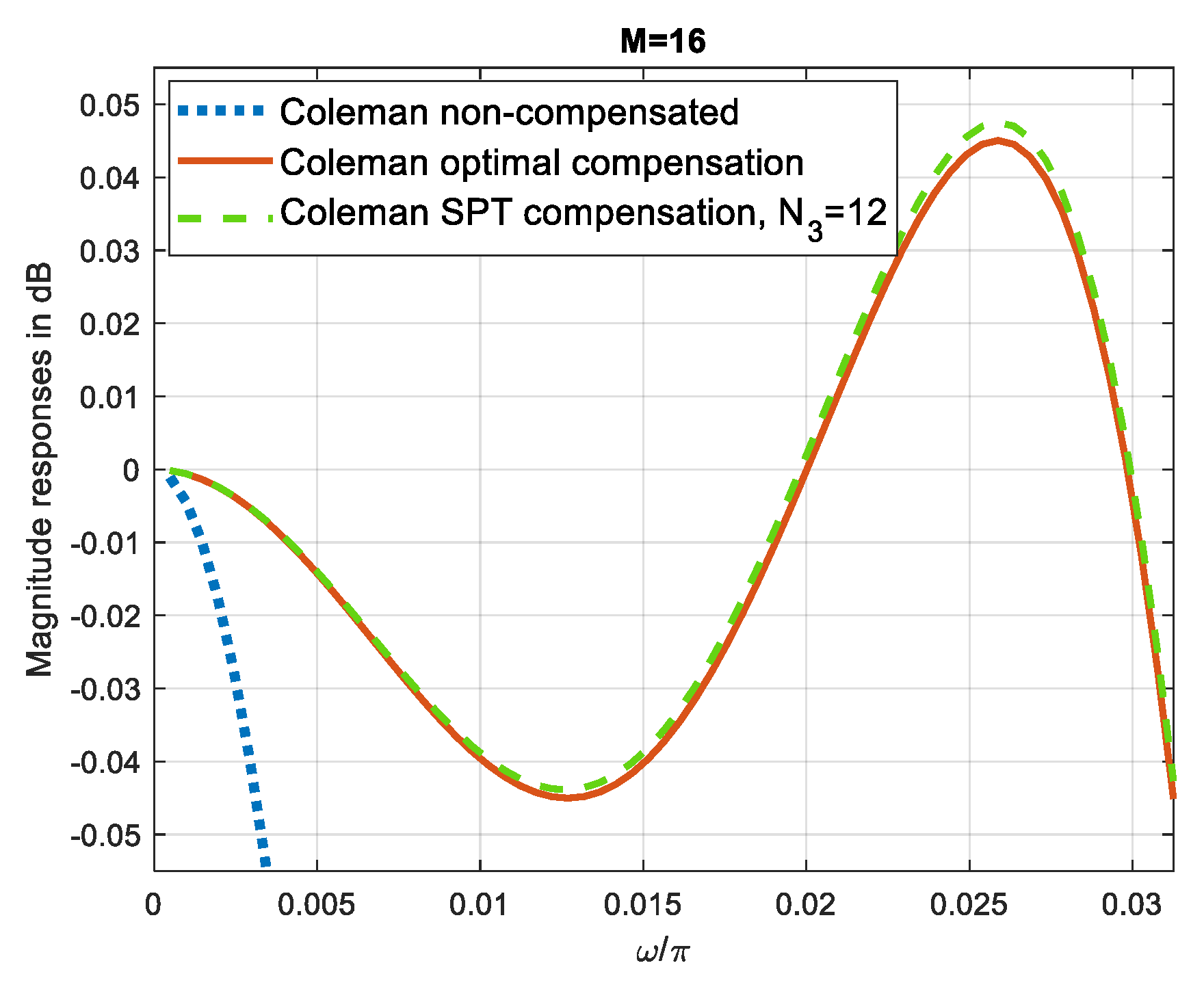
3.2.2. Wideband Compensation

The passband frequency ω_p = 1/2M, and M = 16.

• Compensator C₂

We first consider the compensator C₂ from (6). The optimal compensator coefficients are C_21o = 0.7904 and C_22o = 0.8596, resulting in δ_o = 0.0239 dB. The corresponding SPT coefficients are shown in

Table 2. SPT compensator C₂ coefficients, passband deviations and the number of adders.

C21	C22	δ2 [dB]	N2
20-2−2	20-2−3	0.1232	11
20-2−2 + 2−5	20-2−3	0.0307	12
20-2−2 + 2−5	20-2−3 + 2−7	0.0297	13
20-2−2 + 2−5 + 2−8	20-2−3-2−10	0.0271	14
20-2−2 + 2−5 + 2−7	20-2−3-2−6 + 2−8	0.0247	15

. It can be observed that, with fifteen adders, we have approximately optimum compensation.

Figure 2 contrasts the passband magnitude responses of the Coleman non-compensated, optimum compensated and the SPT compensated with N₂ = 12.

• Compensator C₃

The optimal compensator coefficients are C_31o = 0.7250 and C_32o = 1.3138, resulting in δ_o = 0.045 dB. The corresponding SPT coefficients are shown in

Table 3. SPT compensator C₃ coefficients, passband deviations and the number of adders.

C31	C32	δ3 [dB]	N3
20-2−2	20-2−2 + 2−6	0.0616	9
20-2−2-2−8	20-2−2 + 2−6	0.0532	11
20-2−2-2−5 + 2−7	20 + 2−2 + 2−4	0.0474	12
20-2−2-2−5 + 2−7	20 + 2−2 + 2−4-2−9	0.04591	13
20-2−2-2−5 + 2−7-2−10	20-2−2 + 2−4-2−14	0.0452	16

. We obtain approximately optimum compensation with thirteen and sixteen adders.

Figure 3 compares the Coleman non-compensated filter passbands, compensated with the optimum filter and compensated with the SPT filter, N₃ = 12.

The corresponding MATLAB programs are given in the Supplementary Material.

3.3. Chebyshev Sharpened Comb Filters [10,11]

We consider M = 20 and Chebyshev polynomial from [10,11],

p(x) = 1 − 2⁹x² + 2¹⁵x⁴,

(13)

where x is a comb filter (1)

$$x=H\left(z,1, 20\right)$$

(14)

3.3.1. Narrowband Compensation

We chose ω_p = 0.22π/M and the compensator C₁ in (3). The optimum parameter C_11o = 0.7213, and δ_o = 0.0111dB. The SPT coefficients are given in

Table 4. SPT compensator C₁ coefficients, passband deviation and the number of adders.

C11	δ1 [dB]	N1
20-2−2	0.0299	4
20-2−2-2−5	0.0125	6
20-2−2-2−5-2−8	0.0115	7
20-2−2-2−5-2−8 + 2−11	0.0110	8

, changing N₁ from four to eight. For N₁ = 8, we obtain approximately the optimum compensation.

Figure 4 compares the passbands of the Chebyshev sharpened non-compensated comb filter, compensated with the optimum filter C₁ and compensated with the SPT compensator C₁ with N₁ = 4.

3.3.2. Wideband Compensation

The passband frequency ω_p = π/2M, while the decimation factor M and the Chebyshev sharpening polynomial are the same as in Section 3.2.1. We will consider the wideband compensators C₂ and C₃.

• Compensator C₂

The optimum values of the compensator parameters obtained using the PSO method are C_21o = 0.6337 and C_22o = 0.6264, while the passband deviation equals δ_o = 0.0171 dB. To obtain a multiplierless design, the optimum parameter values are presented in the SPT form and the results are shown in

Table 5. SPT compensator C₂ coefficients, passband deviations and the number of adders.

C21	C22	δ2 [dB]	N2
2−1 + 2−3	2−1 + 2−3	0.0485	11
2−1 + 2−3 + 2−7	2−1 + 2−3	0.0227	12
2−1 + 2−3 + 2−7	2−1 + 2−3 + 2−8	0.00177	13
2−1 + 2−3 + 2−7 + 2−11	2−1 + 2−3 + 2−9	0.0174	14
2−1 + 2−3 + 2−7 + 2−10	2−1 + 2−3 + 2−10 + 2−12	0.0172	15

. It can be observed that with N₂ = 15 we can obtain almost optimum compensation.

Figure 5 contrasts the magnitude responses in passband of the non-compensated, optimum compensated and the SPT compensated (N₂ = 12) Chebyshev sharpened comb filter [11].

• Compensator C₃

The optimum parameters are obtained using PSO, resulting in C_21o = 0.5946, C_22o = 0.8939 and δ_2o = 0.0302 dB. The SPT parameter values are given in

Table 6. SPT compensator C₃ coefficients, passband deviations and the number of adders.

C31	C32	δ3 [dB]	N
2−1-2−4	20-2−4	0.0597	9
2−1 + 2−4-2−6	20-2−4	0.0404	10
2−1 + 2−3 + 2−6	20-2−3-2−6	0.0373	9
2−1 + 2−3-2−5 + 2−9	20-2−3 + 2−6	0.0317	13
2−1 + 2−3-2−5 + 2−11	20-2−3 + 2−6 + 2−8	0.0304	14

, along with the corresponding passband deviations and the number of compensator adders.

As observed in Table 6, the approximate optimal optimization can be obtained with N₃ = 14.

Figure 6 compares the passband magnitude responses of the Chebyshev comb filter [11], non-compensated, compensated with the optimal C₃ filter and compensated with the SPT C₃ filter with N₃ = 10.

4. Results

In this section, we first compare the proposed method with the methods in the literature to show its benefits. Next, we summarize the principal features of the proposed design. Finally, we present possible practical applications and introduce potential future work.

4.1. Comparisons

Only a few works propose compensators for Chebyshev sharpening combs [10,11,12]. However, we also include a comparison with one of the most recent works, in which another type of sharpening is applied to improve the passband and stopband of comb filters.

4.1.1. Comparison with Method in [10]

In Table 1 [10], the authors proposed four compensated Chebyshev sharpened combs. In continuation, we then present a comparison of all the cases.

• Chebyshev sharpening polynomial p(x) = 1 − 2⁹x + 2¹⁵x², x = H(z, 1, 32)

The passband edge is ω_p = 0.226π/M where M = 32. The design in [10] requires N = 9 adders, resulting in δ_p = 0.06 dB. We used the narrowband compensator C₁. The PSO design results in C_11o = 0.3549 and δo = 0.0043 dB. The SPT design results are shown in

Table 7. SPT compensator C₁ coefficients, passband deviation and the number of adders.

C11	δ1 [dB]	N1
2−1-2−3	0.0169	4
2−1-2−3-2−6	0.0064	5
2−1-2−3-2−6-2−8	0.0045	6
2−1-2−3-2−6-2−8-2−11	0.0043	7

.

The results in Table 7 highlight the efficiency of the proposed designs (denoted in bold), which outperform those in [10], requiring fewer adders and providing better compensation.

• Chebyshev Sharpening Polynomial p(x) = 1 − 2¹⁰x + 2¹⁷x², x = H(z, 1, 32)

The passband edge is ω_p = 0.164π/M where M = 32. The design in [10] requires N = 8 adders, resulting in δ_p = 0.02 dB. In the proposed design, we choose the compensator C₁. The optimum PSO design gives C_11o = 0.3443 and δo = 0.0012 dB. The results of the SPT design are shown in

Table 8. SPT compensator C₁ coefficients, passband deviation and the number of adders.

C11	δ1 [dB]	N1
2−1-2−3	0.0157	4
2−1-2−3-2−5	0.0015	5
2−1-2−3-2−5-2−11	0.0012	6

.

The proposed designs (denoted in bold) confidently present superior compensation, requiring fewer adders.

• Chebyshev sharpening polynomial p(x) = −1 + 27(2⁶x − 2¹⁴x² + 2²⁰x³), x = H(z, 1, 32)

The passband frequency equals ω_p = 0.187π/M and M = 32 resulting in N = 13 adders and δ_p = 0.05 dB in the design [10]. We applied the compensator C₁ and the PSO design, obtaining C_11o = 0.5248 and δo = 0.0034 dB. The results of the SPT design are shown in

Table 9. SPT compensator C₁ coefficients, passband deviation and the number of adders.

C11	δ1 [dB]	N1
2−1 + 2−5	0.0056	4
2−1 + 2−5-2−8	0.0042	5
2−1 + 2−5-2−7 + 2−9	0.0036	6
2−1 + 2−5-2−7 + 2−9-2−11	0.0035	7

.

Once again, the proposed design shown in Table 9 reassures us with its significantly improved compensation and fewer adders.

• Chebyshev sharpening polynomial p(x) = −1 + 27(2⁴x − 2¹⁰x² + 2¹⁴x³), x = H(z, 1, 32)

The passband edge equals ω_p = 0.354π/M and M = 32. The design in [10] resulted in N = 13 adders and δ_p = 0.05 dB. In our design, we chose the wideband compensator C₃. The PSO design results in C_31o = 0.4998, C_32o = 0.4300 and δ_o = 0.0023 dB, while the results of the SPT design are shown in

Table 10. SPT compensator C₃ coefficients, passband deviations and the number of adders.

C31	C32	δ3 [dB]	N3
2−1-2−13	2−1-2−4	0.0101	9
2−1-2−13-2−16	2−1-2−4	0.0100	11
2−1-2−11-2−13	2−1-2−4 + 2−10	0.0098	12

.

In Table 10, presented in bold, the proposed design demonstrates better compensation and fewer adders in all cases.

Additionally, all compensators in [10] need the normalization factor.

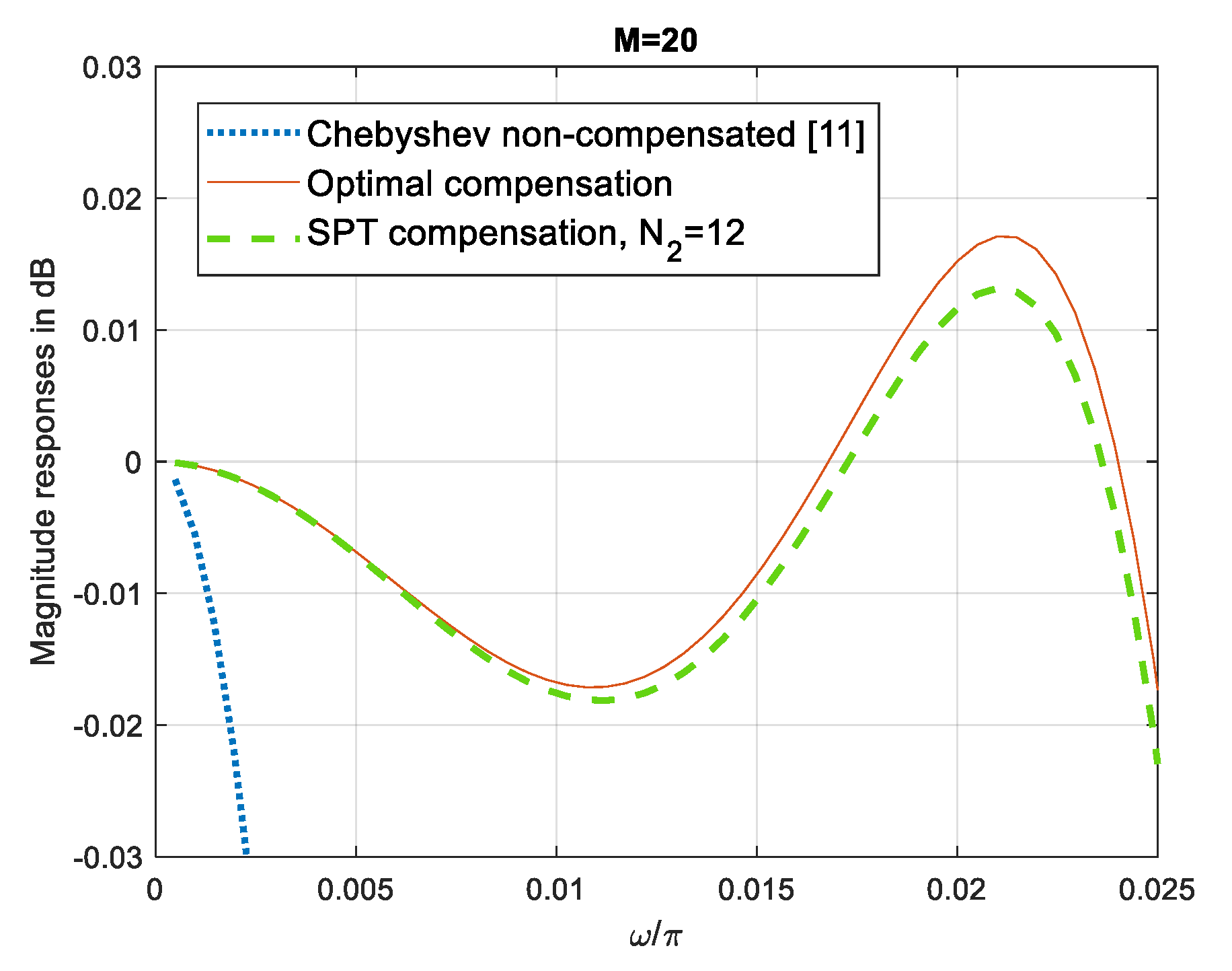
4.1.2. Comparison with Method in [11]

The authors in [11] proposed four Chebyshev sharpened combs and the corresponding optimum compensator designs to improve the passband while keeping the number of adders as low as possible. We compare our designs, taking narrowband and wideband cases.

• Chebyshev sharpening polynomial p(x) = 1 − 2⁹x² + 2¹⁵x⁴, x = H(z, 1, 32)

The passband edge equals ω_p = 0.226π/M where M = 32. The design in [11] requires N = 3 adders resulting in δ_p = 0.02 dB. In our design, we chose the narrowband compensator C₁. The results of the PSO design are C_11o = 0.3543 and δ₁o = 0.0043 dB, while the results of the SPT design are shown in

Table 11. SPT compensator C₁ coefficient, passband deviations and the number of adders.

C11	δ1 [dB]	N1
2−1-2−3	0.0169	4
2−1-2−3-2−6	0.0064	5
2−1-2−3-2−6-2−8	0.0045	6
2−1-2−3-2−6-2−8-2−11	0.0043	7

.

The proposed design offers better compensation requiring more adders. As shown in the first row of Table 11, the proposed design exhibits better compensation at the expense of one additional adder. Unlike [11], the proposed design’s flexibility offers further advantages and improved passband compensation by slightly increasing the adders.

• Chebyshev sharpening polynomial p(x) = −1 + 27(2⁴x − 2¹⁰x² + 2¹⁴x³), x = H(z, 1, 32)

The passband edge equals ω_p = 0.483π/M and M = 32. The optimum design in [11] requires N = 7 adders, resulting in δ_p = 0.12 dB. Since C₃ requires fewer adders than C₂, we apply the wideband compensator C₃ in our design. The results of the optimal PSO design are C_31o = 0.8888, C_32o = 1.8668 and δ_3o = 0.0554 dB, while the SPT design results are given in

Table 12. SPT compensator C₃ coefficients, passband deviations and the number of adders.

C31	C32	δ3 [dB]	N3
20-2−3	21-2−3	0.0776	9
20-2−3 + 2−7	21-2−3	0.0601	11
20-2−3 + 2−6-2−9	21-2−3-2−7	0.0587	13
20-2−3 + 2−6 + 2−9	21-2−2 + 2−4 + 2−7	0.0555	16

.

The proposed design in the first row of Table 12 exhibits much better compensation, requiring two additional adders. Unlike [11], other results in Table 12 offer a trade-off between improving compensation and slightly increasing the number of adders. Additionally, all compensators in [11] need the normalization factor.

4.1.3. Comparison with Method in [12]

We compare our design with Example 2 in [12], where the compensator for Chebyshev sharpening polynomial p(x) = −1 + 27(2³x² − 2⁸x⁴ + 2¹¹x⁶), x = H(z, 1, 32), is designed. The design’s results are given in Table II in [12]. Our design, meticulously presented in

Table 13. SPT compensator C₂ coefficients, passband deviations and the number of adders.

C21	C22	δ2 [dB]	N2
2−1 + 2−5	2−2 + 2−6	0.0307	11
2−1-2−5 + 2−8	2−1 + 2−7	0.0276	12
2−1-2−5 + 2−8	2−1 + 2−7 + 2−9	0.0273	13
2−1-2−5 + 2−8 + 2−10	2−1 + 2−7-2−11	0.0266	14
2−1 + 2−5 + 2−7-2−9-2−11	2−1 + 2−7-2−9 + 2−11	0.0262	16

, provides a clear comparison. For N₂ = 11, the passband deviation equals 0.0307 dB, compared to 0.0587 dB, which needed the same number of adders as shown in the third row of Table 2 in [12]. Further increase in the number of adders, a key design parameter, results in a decrease of the passband deviation, as shown in Table 13. This relationship demonstrates the design’s ability to improve performance with a slightly increased number of adders.

4.1.4. Comparison with Method in [7]

In [7], a two-stage comb decimation filter with a sharpened comb in the second stage was proposed. A linear optimization technique determines the coefficients of sharpening polynomial. The complexity of the design expressed in the number of adders per output sample (APOS) equals 163, while the minimum stopband attenuation is 30 dB, and the passband deviation is 0.16 dB. This work is compared in [7] with the compensated Chebyshev sharpening comb using polynomial p(x) = 1 − 2⁹x² + 2¹⁵x⁴ [11] for ω_p = 0.226π/M and M = 32. This filter requires 138 APOS with a minimum stopband attenuation of 38.12 dB and a passband deviation of 0.02 dB.

The proposed compensator from the first row in Table 11 is applied to the Chebyshev sharpened comb, resulting in a passband deviation of 0.0169 dB and the number of APOS equals 139, which is a much better result than in [7].

4.2. Principal Features of the Proposed Method

The principal features of the proposed method to improve the passband of the Chebyshev sharpened comb filters from the literature are summarized as follows:

• The method includes the compensation of Coleman Chebyshev comb filters, which have a favorite characteristic of providing high and equal attenuations in all folding bands.
• The choice of narrowband and wideband compensators depends on the passband of interest. For the wideband case, there is a choice between two compensators depending on the number of adders and the compensation quality.
• All designs have the option of optimal multiplier and multiplierless designs.
• Design flexibility presented as a trade-off between the number of adders and the quality of compensations.
• Simplicity of design since there is only one parameter in the narrowband case and two parameters in the wideband case to optimize.
• The comparisons with the methods from the literature demonstrate the advantages of the proposed method.

4.3. Possible Practical Applications

Compensated Chebyshev decimation filters, a class of digital filters designed to provide accurate signal decimation while compensating for the effects of Chebyshev filters, such as passband droop, are particularly valuable in applications where maintaining high signal fidelity during decimation is of utmost importance. Here are some possible practical implementations:

• Communication Systems. Providing efficient decimation since the signals are often decimated to match a target sampling rate. In radio frequency (RF) signal processing, these filters can significantly improve the performance of intermediate frequency (IF) decimation stages by reducing signal distortion and improving signal-to-noise ratio.
• Biomedical Signal Processing. These filters can be used to decimate high-frequency sampled biomedical signals to preserve signal information by accurately retaining the key features of the original signal while reducing the data rate.
• Audio Signal Processing. To maintain high sound quality during resampling or multi-rate processing, minimize aliasing and maintain audio integrity.
• Scientific Instrumentation. Preservation signal quality in high-resolution imaging or spectroscopy applications. Accurate decimation of geophysical signals aids in the real-time monitoring and analysis of seismic data.

4.4. Potential Future Research Work

Compensated Chebyshev sharpened decimation filters can become even more versatile and effective in modern signal processing domains by focusing on various applications and research areas. A key aspect of this is ensuring robustness to various input signal conditions, a challenge that is crucial for the practicality of the research. Other key challenges for future work include achieving optimal trade-offs between computational complexity and performance, and addressing hardware constraints in real-time systems.

Integration with Machine Learning. Exploring the synergy of compensated Chebyshev sharpened decimators with machine learning algorithms to dynamically adjust parameters based on historical or expected input signal statistics—training models to fine-tune filter coefficients in real time for non-stationary signals.

Advanced Compensation Techniques. The need for filters that dynamically adapt their compensation based on real-time signal characteristics or varying decimation factors is crucial. Exploring methods to handle signals with nonlinear distortions or dynamics is a key aspect of this research.

Implementation Optimization. Design hardware-efficient algorithms for FPGA or ASIC implementations to optimize power and speed. Investigate approaches for real-time, high-throughput system implementation.

References

1. Kaiser, J.; Hamming, R. Sharpening the response of a symmetric non-recursive filter by multiple use of the same filter. IEEE Trans. Acoust. Speech Signal Process 1977, 25, 415–422. [Google Scholar] [CrossRef]
2. Kwentus, A.Y.; Zhongnong, J.; Willson, A.N. Application of filter sharpening to cascaded integrator-comb decimation filters. IEEE Trans. Signal Process 1997, 45, 457–467. [Google Scholar] [CrossRef]
3. Neeraja, P.K.; Bindiya, T.S.; Ragh, C.W. Low Power Implementation of Compensated and Sharpened CIC Decimation Filter. In Proceedings of the IEEE 9th Uttar Pradesh International Conference on Electrical, Electronics and Computer Engineering (UPCON 2022), Allahabad, India, 2–4 December 2022. [Google Scholar] [CrossRef]
4. Dudarin, A.; Goran Molnar, G.; Vucic, M. Optimum multiplierless sharpened cascaded-integrator-comb filters. Dig Sig. Proc 2022, 127, 103564. [Google Scholar] [CrossRef]
5. Aggarwal, S. Efficient design of decimation filter using linear programming and its FPGA implementation. Integration 2021, 79, 94–106. [Google Scholar] [CrossRef]
6. Aggarwal, S.; Meher, P.K. Enhanced sharpening of CIC decimation filters implementation and applications. Circ. Syst. Signal Proc. 2022, 41, 4581–4603. [Google Scholar] [CrossRef]
7. Gautam, D.; Khare, K.; Shrivastava, B.P. A novel approach for optimal design of sample rate conversion filter using linear optimization technique. IEEE Access 2021, 9, 44436–44444. [Google Scholar] [CrossRef]
8. Coleman, J.O. Chebyshev stopbands for CIC decimation filters and CIC-implemented array tapers in 1D and 2D. IEEE Trans. Circ. Syst. I Reg. Pap. 2012, 59, 2956–2968. [Google Scholar] [CrossRef]
9. Molnar, G.; Dudarin, A.; Vucic, M. Minimax design of multiplierless sharpened CIC filters based on interval analysis. In Proceedings of the 39th International Convention on Information and Communication Technology, Electronics and Microelectronics, (MIPRO 2016), Opatija, Croatia, 30 May–3 June 2016; pp. 94–98. [Google Scholar] [CrossRef]
10. Molnar, G.; Dudarin, A.; Vucic, M. Design and multiplierless realization of maximally flat sharpened-CIC compensators. IEEE Trans. Circ. Syst. II Express Briefs 2018, 65, 51–55. [Google Scholar] [CrossRef]
11. Dudarin, A.; Molnar, G.; Vucic, M. Optimum multiplierless compensators for sharpened cascaded-integrator-comb decimation filters. Electron. Lett. 2018, 54, 971–972. [Google Scholar] [CrossRef]
12. Jovanovic Dolecek, G.; Martinez Novelo, G. Design of compensator for Chebyshev sharpened comb filter. In Proceedings of the 2023 IEEE 33rd International Conference on Microelectronics (MIEL), Nis, Serbia, 16–18 October 2023. [Google Scholar] [CrossRef]
13. Jovanovic Dolecek, G.; Fernandez-Vazquez, A. Trigonometrical approach to design a simple wideband comb compensator. AEU-Int. J. Electron. Commun. 2014, 68, 437–441. [Google Scholar] [CrossRef]
14. Jovanovic Dolecek, G.; Garcia Baez, R.; Molina Salgado, G.; de la Rosa, J.M. Novel multiplierless wideband comb compensator with high compensation capability. Circ. Syst. Signal Proc. 2017, 36, 2031–2049. [Google Scholar] [CrossRef]
15. Jovanovic Dolecek, G.; de la Rosa, J.M. Design of wideband comb compensator based on magnitude response using two sinusoidals and particle swarm optimization. AEU-Int. J. Electron. Commun. 2021, 130, 153570. [Google Scholar] [CrossRef]
16. Xu, L.; Yang, L.W.; Tian, H. Design of wideband CIC compensator based on particle swarm optimization. Circ. Syst. Signal Proc. 2019, 38, 1833–1846. [Google Scholar] [CrossRef]
17. Zhibin, L.; Ruotong, Y.; Min, G. Efficient sharpening CIC filter embedding fifth-order filter with coefficient optimisation algorithm. Electron. Lett. 2020, 56, 1241–1243. [Google Scholar] [CrossRef]
18. Harris, F. Multirate Signal Processing for Communications Systems; River Publisher: Gistrup, Denmark, 2021. [Google Scholar]
19. Milic, L.J. Multirate Filtering for Digital Signal Processing; IGI Global: Hershey, PA, USA, 2009. [Google Scholar]
20. de la Rosa, J.M. Sigma-Delta Converters, Practical Design Guide, 2nd ed.; Wiley-IEEE Press: New Jersey, NY, USA, 2018; pp. 20–27. [Google Scholar]
21. Tobin, P. PSpice for Digital Signal Processing. Synthesis Lectures on Digital Circuits & Systems; Springer: Cham, Switzerland, 2007; pp. 109–131. [Google Scholar] [CrossRef]
22. White, B.A.; Elmasri, M.I. Low-power design of decimation filters for a digital IF receiver. IEEE Trans. Very Large Scale Integr. (Vlsi) Syst. 2000, 8, 339–345. [Google Scholar] [CrossRef]
23. Abinaya, A.; Maheswari, M. A survey of digital down converter architecture for next generation wireless applications. Proc. Iop Conf. Ser. Mater. Sci. Eng. 2000, 872, 012037. [Google Scholar] [CrossRef]
24. Chukwuchekwa, N. Illustration of Decimation in Digital Signal Processing (DSP) Systems Using MATLAB. 2009. Available online: https://www.researchgate.net/publication/334432641 (accessed on 10 November 2024).
25. Wang, W.; Jin, X.; Quan, D.; Zhu, M.; Wang, X.; Zheng, M.; Li, J.; Chen, J. Rate adaptive compressed sampling based on region division for wireless sensor networks. Sci. Rep. 2024, 14, 1–13. [Google Scholar] [CrossRef]
26. Gan, C.; Li, X. Improved CIC Decimation Filter on Software Defined Radio. In Proceedings of the 2021 9th International Conference on Communications and Broadband Networking (ICCBN 21), Shanghai China, 25–27 February 2021; pp. 232–238. [Google Scholar] [CrossRef]
27. Ainsworth, M.; Klasky, S.; Whitney, B. Compression using lossless decimation analysis and application. SIAM J. Sci. Comput. 2017, 39, B732–B757. [Google Scholar] [CrossRef]
28. Yang, M.; Guerra, R.; Han, C.; López, J.F. A near lossless data compression method for the geostationary interferometric infrared sounder (GIIRS) based on the combination of decimation and quantization. In Proceedings of the IEEE 8th Joint Int Inf Tech and Artific Intell Conf (ITAIC2019), Chongqing, China, 24–26 May 2019. [Google Scholar] [CrossRef]
29. Rahate, T.W.; Ladhake, S.A.; Ghate, U.S. Decimator filter for hearing aid application based on FPGA. Int. Res. J. Eng. Tech. (IRJET) 2018, 5, 1175–1183. [Google Scholar]
30. Lin, L.; Gao, B.; Gong, M. An area-efficient decimation filter on high resolution Sigma Delta A/D converter for biomedical signal processing. In Proceedings of the 2020 IEEE International Conference on Advances in Electrical Engineering and Computer Applications (AEECA), Dalian, China, 25–27 August 2020. [Google Scholar] [CrossRef]
31. Yang, R.; Liu, H.; Luo, Z. Optimization design of decimation filter for the phasemeter in the space gravitational wave detection. IEEE Trans. Inst. Meas. 2024, 73, 1–8. [Google Scholar] [CrossRef]
32. Smalt, C.J.; Brungart, D.S. Digital sampling of acoustic impulse noise: Implications for exposure measurement and damage risk criteria. J. Acoust. Soc. Am. 2022, 152, 1283–1291. [Google Scholar] [CrossRef] [PubMed]
33. Available online: https://www.mathworks.com/help/gads/particleswarm.html (accessed on 15 September 2024).
Figure 1. Compensation of Coleman Chebyshev comb [8], M = 16, with the narrowband filter C1. Overall magnitude responses and passband zooms: (a) Overall magnitude responses of Coleman non-compensated and optimal compensated filters; (b) Passband zoom of Coleman non-compensated, optimal compensated and SPT compensated filters with N1 = 5.
Applsci 14 11421 g001
Figure 2. Compensation of Coleman sharpening filter [8], M = 16, with the wideband filter C2. Passband magnitude responses of non-compensated, optimal compensated and SPT compensated Coleman sharpening comb filters with N2 = 12.
Applsci 14 11421 g002
Figure 3. Wideband compensation of Coleman sharpening filter [8], M = 16, using filter C3. Passband magnitude responses of non-compensated, optimal compensated and SPT compensated Coleman sharpening comb filters, with N3 = 12.
Applsci 14 11421 g003
Figure 4. Compensation of Chebyshev sharpened filter [11], M = 20, with the narrowband compensator C1. Passband magnitude responses of non-compensated, optimal compensated and SPT compensated N1 = 4 filters.
Applsci 14 11421 g004
Figure 5. Compensation of Chebyshev sharpened filter [11], M = 20, with the narrowband compensator C1. Passband magnitude responses of non-compensated, optimal compensated and SPT compensated, N1 = 4, filters.
Applsci 14 11421 g005
Figure 6. Compensation with the wideband compensator C3. Passband magnitude responses of non-compensated, optimal compensated and SPT compensated, N3 = 10, Chebyshev sharpening comb filters [11] with M = 20.
Applsci 14 11421 g006