Research on Risk Quantification Methods for Connected Autonomous Vehicles Based on CNN-LSTM

Abstract

Quantifying and predicting driving risks for connected autonomous vehicles (CAVs) is critical to ensuring the safe operation of traffic in complex environments. This study first establishes a car-following model for CAVs based on molecular force fields. Subsequently, using a convolutional neural network and long short-term Memory (CNN-LSTM) deep-learning model, the future trajectory of the target vehicle is predicted. Risk is quantified by employing models that assess both the collision probability and collision severity, with deep-learning techniques applied for risk classification. Finally, the High-D dataset is used to predict the vehicle trajectory, from which the speed and acceleration of a target vehicle are derived to forecast driving risks. The results indicate that the CNN-LSTM model, when compared with standalone CNN and LSTM models, demonstrates a superior generalization performance, a higher sensitivity to risk changes, and an accuracy rate exceeding 86% for medium- and high-risk predictions. This improved accuracy and efficacy contribute to enhancing the overall safety of connected vehicle platoons.

1. Introduction

With the advancement in intelligent connectivity and vehicle–road coordination technologies, human-like driving in smart vehicles has become a significant area of research. However, this progress has also brought substantial challenges to traffic safety. Predicting and quantifying the driving risks of CAVs is crucial for ensuring safe driving and effectively managing risks. In recent years, research in this field has focused on improving the accuracy of driving risk prediction and quantification.

The current risk quantification methods are mainly divided into two categories: deterministic methods and probabilistic methods. Deterministic methods use predefined thresholds for indicators such as the time to collision (TTC), time to stop (TTS), and time to reaction (TTR) to assess collision risks. Kim et al. [1] applied threat prediction algorithms and the conflict zones of surrounding vehicles to calculate the TTC within a time range, guiding the driving strategy of autonomous vehicles. On the other hand, probabilistic methods consider the spatiotemporal relationships between vehicles and simulate collision risks by incorporating uncertainty factors. Noh et al. [2] and others utilized vehicle-to-vehicle (V2V) communication to predict vehicle positions and assess risk probabilities through Bayesian networks. Li et al. [3] proposed a probabilistic-model-based conditional random field (CRF) situational assessment module to evaluate the risk levels of the surrounding traffic participants. Zheng et al. [4] and others combined the driving risk quantification with an equivalent force model, designing a field model framework for driving risk, which identifies the risks from various directions and implements the corresponding preventive measures.

Research on driving risk prediction and quantification can help identify potential road safety hazards. Xu et al. [5] defined safety risks as ensuring that network decisions are consistent with human perception and proposed a safety attribute to instantiate and quantify these risks. Wang et al. [6] introduced a machine-learning framework to systematically address future driving risks related to collisions, extracting features from records to define five different types of risks.

Precise path planning and risk control can effectively reduce the likelihood of vehicles entering high-risk areas, thereby lowering the incidence of traffic accidents. Moon et al. [7] proposed a multi-objective vehicle path control method based on deep Q-networks, which performs better than existing methods in terms of driving distance, time, and waiting time in dynamic traffic environments. Kong et al. [8] used a multinomial logistic regression model to reveal the choice behaviors of each potential cluster in different interactive driving scenarios, setting higher standards for drivers when changing lanes.

In summary, although extensive research has been conducted on risk prediction and quantification, the current risk prediction and quantification for CAVs generally rely on single-feature models and have not fully considered the impact of multi-feature models. This paper will build upon the CNN and LSTM models, using a CNN-LSTM fusion model to predict the future trajectories of following vehicles. It will integrate two feature models—collision probability and collision severity—to quantify the risks. By calculating the target vehicle’s speed and acceleration, the paper aims to further achieve risk quantification and prediction for connected autonomous vehicles.

2. Car-Following Model for CAVs Based on Molecular Force Fields

2.1. System Similarity Analysis

The interaction between molecules involves forces that govern their relative positions and velocity changes. Similarly, forces exist between vehicles, impacting their relative positions and speeds. The interaction forces between molecules vary with the distance between them; likewise, the interaction between vehicles is impacted by their distance from one another. For instance, when a following vehicle gets closer to the vehicle ahead, it will decelerate to avoid a collision. Conversely, when the following vehicle is farther from the lead vehicle, it will accelerate to close the gap. In molecular systems, equilibrium is reached when the forces between molecules balance, resulting in a stable state for the system. In a similar way, in vehicle models, a dynamic equilibrium between vehicles can be achieved, leading to the stable movement of the entire platoon. Therefore, by exploring the mechanical interactions between molecules, the car-following characteristics of CAVs can be derived and a car-following model for CAVs was developed.

2.2. Car-Following Model for CAVs

Qu et al. [9] expressed the molecular force field potential function as follows:

$$\phi \left(r\right)=\frac{\mathsf{\epsilon }}{\mathsf{\alpha }-\mathsf{\beta }}\left[\mathsf{\beta }{\left(\frac{r_e}{r}\right)}^{\mathsf{\alpha }}-\mathsf{\alpha }{\left(\frac{r_e}{r}\right)}^{\mathsf{\beta }}\right]$$

(1)

where $\phi \left(r\right)$ is the potential energy; $\mathsf{\alpha }$ and $\mathsf{\beta }$ are the constants for repulsive and attractive forces, respectively; $r$ is the distance between molecules; and $\mathsf{\epsilon }$ is the depth of the potential well at equilibrium distance $r_e$.

The force acting on a molecule is derived as follows:

$$F\left(r\right)={\displaystyle \frac{\mathsf{\alpha }\mathsf{\beta }\mathsf{\epsilon }}{\mathsf{\alpha }-\mathsf{\beta }}}\left({\displaystyle \frac{r_e^{\mathsf{\beta }}}{r^{\mathsf{\beta }+1}}}-{\displaystyle \frac{r_e^{\mathsf{\alpha }}}{r^{\mathsf{\alpha }+1}}}\right)$$

(2)

The acceleration model for CAVs based on molecular force fields is then derived as follows:

$$a_z={\displaystyle \frac{\mathsf{\alpha }\mathsf{\beta }\mathsf{\epsilon }}{\mathsf{\alpha }-\mathsf{\beta }}}\left({\displaystyle \frac{s_a^{\mathsf{\beta }}}{l^{\mathsf{\beta }+1}}}-{\displaystyle \frac{s_a^{\mathsf{\alpha }}}{l^{\mathsf{\alpha }+1}}}\right)$$

(3)

where $l$ is the actual distance between the leading and the following vehicles. $s_a$ represents the safe following distance.

3. CAV Trajectory Prediction

Quantifying and predicting the risks of CAVs requires establishing a car-following model and an acceleration model based on molecular force fields. These processes also rely on predicting the future trajectories of vehicles, making deep-learning methods a suitable choice for trajectory prediction. Traditional studies often used vehicle motion models for trajectory prediction, but these models tend to have significant deviations in long-term forecasts. To achieve predictions closer to reality, deep-learning models can be employed. A fusion model that combines the strengths of CNN and LSTM networks enables a more accurate prediction of vehicle trajectories. This integrated model is referred to as the CNN-LSTM model.

In the CNN-LSTM model, the LSTM and CNN components are constructed on two separate paths, ensuring no correlation between them. Figure 1 illustrates the framework of the proposed method. As shown in the figure, the data first pass through both the LSTM and CNN paths for processing. By leveraging the unique characteristics of each model, the required relationships are effectively extracted.

3.1. CNN

CNN is a deep-learning model widely applied in fields such as image processing, computer vision, and natural language processing. Inspired by the biological visual system, it mimics the way the human brain processes visual information to effectively extract features.

The core component of a CNN is the convolutional layer, which processes input data using multiple learnable convolutional kernels. These kernels slide over the input data, extracting features through localized perception. This operation captures local features such as edges and textures in images, facilitating the learning of deeper-level features. The convolutional layer extracts local features through the convolution operation, which is computed as follows:

$$S\left(i,j\right)=\left(C\cdot K\right)\left(i,j\right)={\displaystyle \sum _m{\displaystyle \sum _{n}c\left(i+m,j+n\right)}}\cdot k\left(m,n\right)+a$$

(4)

where $C$ is the input feature; $K$ is the convolutional kernel; and $a$ is the bias term.

The convolutional layer is typically followed by a pooling layer, which reduces the dimensionality of the data through sampling, thereby decreasing the computational complexity while preserving the information quality. It also enhances the model’s robustness to small shifts and rotations in the input data. In this work, multiple features are mapped to a single feature, then weighted by $k_{x+1}$, and a bias term $a_{x+1}$ is added.

The output of the $\mathrm{k}$th convolutional layer can be calculated as follows:

$$c_k^{\mathrm{u}}=f\left({\displaystyle \sum _i{x}_{k-1}^i}\cdot J_k^{ij}+b\right)$$

(5)

where $f$ is the activation function; $J_k^{ij}$ is the convolutional kernel; $b$ is the additive bias corresponding to the $\mathrm{t}$th feature value; and $x_{k-1}^i$ is the output of the ($k-1)\mathrm{t}\mathrm{h}$ convolutional layer. Constraints: $\mathrm{i}\in \left[1,\mathrm{N}\right]$, represents the number of input feature maps; $j\in \left[1,\mathrm{M}\right]$ denotes the size of the convolutional kernel; $u\in \left[1,\mathrm{U}\right]$ indicates the number of output feature maps; and $k$ represents the current layer of the convolutional network.

The rectified linear unit (ReLU) is a widely used nonlinear activation function that effectively reduces complexity while preserving most of the data’s activation, thereby enhancing training performance. ReLU is defined as follows:

$$\mathrm{Re}LU=\left\{\begin{array}{l}x,x>0\\ 0,x\le 0\end{array}\right\}$$

(6)

Since the gradient in the non-negative region is constant, the vanishing gradient problem does not occur with ReLU, which helps the model maintain a steady convergence rate.

3.2. LSTM Network

The LSTM is a specialized type of recurrent neural network (RNN) primarily designed for handling and predicting time-series data as well as dependencies within sequences. Traditional RNNs often encounter issues such as vanishing or exploding gradients when processing long sequences, making it difficult to learn long-term dependencies. The LSTM addresses this challenge through a series of unique structural designs, effectively overcoming these limitations.

The LSTM can effectively retain important long-term information while discarding unnecessary data, allowing it to process sequences of varying lengths more flexibly.

The Flatten layer is used to convert multi-dimensional input into a one-dimensional array. It transforms the data into a one-dimensional vector so that it can be processed by subsequent fully connected layers.

The fully connected layer is located at the final stage, receiving the features output by the previous CNN and LSTM layers. Each neuron in the fully connected layer is connected to all neurons from the previous layers, integrating various features to perform classification tasks. The ReLU activation function is also used in the fully connected layer to help the model capture complex patterns.

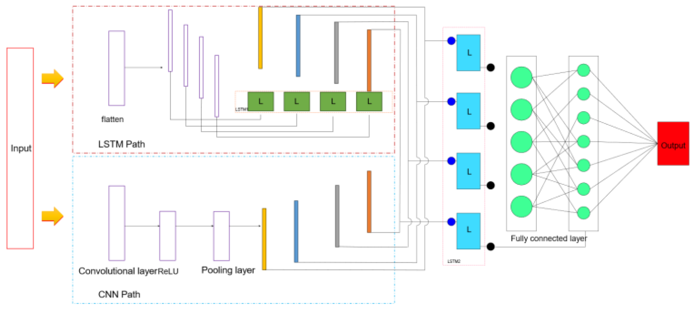
3.3. Trajectory Prediction Model

By analyzing the historical trajectories of the surrounding vehicles and the target vehicle, the future trajectory of the target vehicle can be predicted. As shown in Figure 2, Figure 3 and Figure 4, the historical trajectory of each vehicle is represented by a line segment from its rear. The past trajectories of the target vehicle and surrounding vehicles are shown in blue and yellow, respectively, while the predicted acceleration trajectory is shown in green, and the deceleration trajectory is marked in red.

The surrounding vehicles considered include the lead vehicle, left–front vehicle, right–front vehicle, rear vehicle, left–rear vehicle, and right–rear vehicle, as well as the closest neighboring vehicles in adjacent lanes along the longitudinal direction. All nine historical trajectories are input into the model:

$$J_t=\left\{j_t^1,j_t^2,\cdot \cdot \cdot ,j_t^9\right\}$$

(7)

$$j_t^i=\left\{\left(x_{t-n_h\cdot \Delta t1}^i,y_{t-n_h\cdot \Delta t1}^i\right),\left(x_{t-\left(n_h-1\right)\cdot \Delta t1}^i,y_{t-\left(n_h-1\right)\cdot \Delta t1}^i\right),\cdot \cdot \cdot ,\left(x_t^i,y_t^i\right)\right\}$$

(8)

where $j_t^i$ is the historical trajectory of the vehicle $i$ at time $t$ and $∆t_1=0.2 \mathrm{s}$.

The output is the future trajectory of the target vehicle:

$$D_t=\left\{\left(x_{t+1\cdot \Delta t_2},y_{t+1\cdot \Delta t_2}\right),\left(x_{t+2\cdot \Delta t_2},y_{t+2\cdot \Delta t_2}\right),\cdot \cdot \cdot \left(x_{t+n\cdot \Delta t_2},y_{t+n\cdot \Delta t_2}\right)\right\}$$

(9)

where $∆t_2=0.5 \mathrm{s}$.

4. CAV Driving Risk Quantification Model

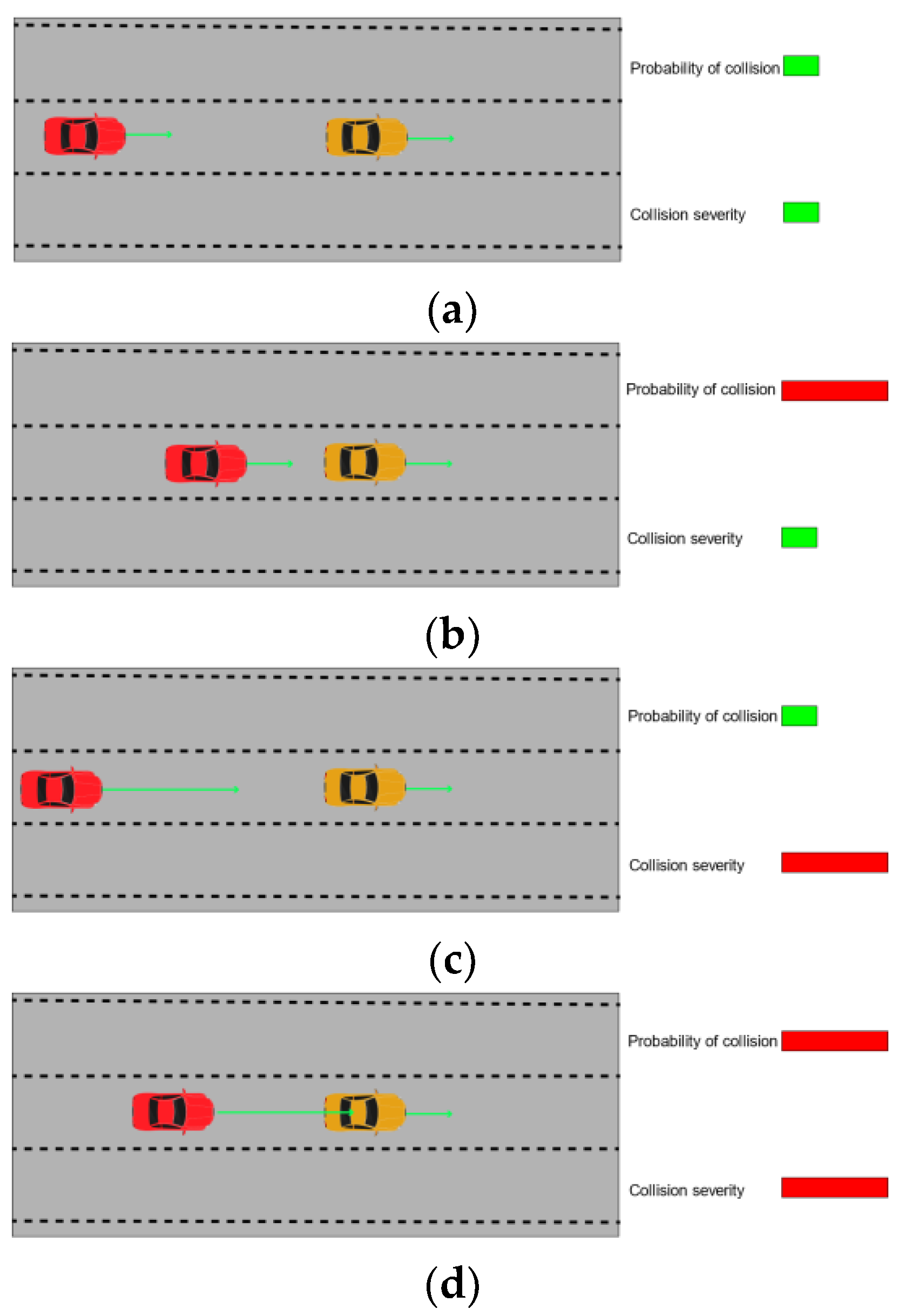
4.1. Time-to-Collision Adjustment

Surrogate safety measures (SSMs) are used to identify near-collision or collision-like events [10]. One of the most commonly used SSMs for rear-end collisions is the TTC. The TTC is defined as the remaining time before two vehicles collide, assuming their current speeds and trajectories remain unchanged throughout the process [11].

$$TTC={\displaystyle \frac{X}{v_h-v_q}},v_h>v_q$$

(10)

where $X=x_q-x_h-{l_q, ∆v=v_h-v_q,x}_q,v_q,\mathrm{a}\mathrm{n}\mathrm{d} {\mathrm{l}}_{\mathrm{q}}$ are the position, speed, and length of the lead vehicle, respectively; while ${\mathrm{x}}_{\mathrm{h}} \mathrm{a}\mathrm{n}\mathrm{d} {\mathrm{v}}_{\mathrm{h}}$ are the position and speed of the following vehicle.

The TTC is only meaningful when the following vehicle is moving faster than the lead vehicle. To address this limitation, Ozbay et al. [12] proposed the modified time to collision (MTTC), which takes into account the accelerations of both the lead and following vehicles, as well as their relative speed.

$$t_{1,}{t}_2={\displaystyle \frac{-\Delta v\pm \sqrt{\Delta v^2+2\Delta aX}}{\Delta a}},\Delta a\ne 0$$

(11)

$$MTTC=\left\{\begin{array}{l}\begin{array}{cc}\min \left(t_1,t_2\right)& ,t_1>0,t_2>0\end{array}\\ \begin{array}{cc}\max \left(t_1,t_2\right)& ,t_1\cdot t_2<0\end{array}\\ \begin{array}{cc}\begin{array}{cc}\begin{array}{cc}\begin{array}{cc} & {\displaystyle \frac{X}{\Delta v}}\end{array}& \end{array}& ,\Delta a=0\end{array}& \end{array}\end{array}\right\}$$

(12)

where $∆a=a_h-a_q$ and $t_1 \mathrm{a}\mathrm{n}\mathrm{d} {\mathrm{t}}_2$ are the two roots of Equation (11).

4.2. Collision Probability

When vehicles are traveling at similar low speeds or are far apart, the likelihood of a collision and its potential severity are relatively low (Figure 5a). However, when the MTTC value is low and the vehicle is traveling at a relatively low speed, the probability of a collision increases, although the severity remains low (Figure 5b). In contrast, if the following vehicle is traveling at a higher speed with a significant relative velocity, the potential severity of a rear-end collision becomes greater (Figure 5c). Finally, as the following vehicle approaches the lead vehicle with a large speed differential, the worst-case scenario emerges, characterized by both a high collision probability and high severity (Figure 5d).

The MTTC is selected as the metric for calculating the collision probability because, compared to the TTC, the MTTC can encompass a wider range of collision scenarios. At each time step, the MTTC between the target vehicle and the lead vehicle is calculated. The collision probability function is a monotonically decreasing function of the MTTC, meaning that, as the MTTC increases, the likelihood of a collision should decrease, and vice versa. The collision probability is defined as a negative exponential function of the MTTC:

$$P=\left\{\begin{array}{l}\begin{array}{cc}\exp \left(-{\displaystyle \frac{MTTC}{\eta }}\right)& ,p_q=1,MTTC>0\end{array}\\ \begin{array}{cc} & \begin{array}{cc}\begin{array}{cc}\begin{array}{cc} & 0\end{array}& \end{array}& \begin{array}{cc} & ,p_q=0\end{array}\end{array}\end{array}\end{array}\right\}$$

(13)

where $P$ represents the collision probability; $p_q=1$ indicates the presence of a vehicle ahead; $p_q=0$ indicates the absence of a vehicle ahead; and $\eta$ is the decay parameter of the collision probability function. The smaller the value of $\eta$, the faster the decay of $P$ in the equation, and vice versa. In [13], $\eta \in \left[\mathrm{3.5,4.5}\right]$ achieves a high correlation between the simulated collision risks and actual collisions. Within this range, $\eta =3.5 \mathrm{s}$ was selected.

By summing the collision probabilities of all vehicles observed within the time interval, the comprehensive collision probability index $P_z$ is obtained (Equation (14)). The resulting $P_z$ is then divided by the sum of $\theta$, yielding the average collision probability (ACP) for each vehicle over the given time segment (Equation (15)).

$$P_z={\displaystyle \sum _i^n{\displaystyle \sum _{t_a}^{t_b}\left(P\cdot \theta \right)}}$$

(14)

$$ACP={\displaystyle \frac{P_z}{{\displaystyle {\sum }_i^n{\displaystyle {\sum }_{t_a}^{t_b}\left(\theta \right)}}}}$$

(15)

where $\left(t_a,t_b\right)$ is the observation time period and $\mathrm{n}$ is the total number of vehicles within the observation period. According to [14], $\theta$ is a binary function: If and only if the vehicle appears within the observation time period and maintains either a lane-changing or car-following state, $\theta =1$; otherwise, $\theta =0$.

4.3. Collision Severity

To measure the severity of a collision, a collision severity index is introduced as a proxy for the impact of rear-end collisions. In specific situations, the potential impact of a rear-end collision is determined by the product of the following vehicle’s speed and the speed difference between the following and leading vehicles.

$$CS=\left\{\begin{array}{l}\begin{array}{cc}\omega \cdot v_q\cdot \left(v_q-v_h\right)& ,p_q=1,\left|x_h-x_q\right|<l\end{array}\\ \begin{array}{cc}\begin{array}{cc}\begin{array}{cc}\begin{array}{cc}\begin{array}{cc} & \end{array}& -\infty \end{array}& \end{array}& ,p_q=0\end{array}& \end{array}\end{array}\right\}$$

(16)

where $\omega$ is a proportional factor that includes vehicle-specific collision factors such as the vehicle’s size, mass, and color; and $\mathrm{l}$ is the threshold distance, beyond which the lead and following vehicles are far enough apart that the collision severity no longer exists. The value of $\mathrm{l}$ should be sufficiently large to account for all possible accidents, and it may depend on factors such as the speed limit of the road and other conditions.

$\omega =1$ is used to account for the impact of all vehicle-specific factors. ${CS}_l$ is defined as the limiting value of $CS$, which is used to normalize the $CS$ to avoid large values in the calculation. ${CS}_l$ corresponds to the scenario where the vehicle is traveling at the speed limit of the road, while the lead vehicle is stationary.

$$C{S}_l=v_l^2$$

(17)

where $v_l$ is the speed limit on the road.

The collision severity is modeled as a monotonically increasing function of $CS$, since an increase in the following vehicle’s speed and relative speed results in a greater severity, and vice versa. Based on [15], the risk of pedestrian fatalities increases monotonically with the vehicle collision speed. A positive exponential function is used to describe this monotonic growth and to calculate the collision severity:

$$Q=\exp \left({\displaystyle \frac{CS}{C{S}_L}}\right)$$

(18)

where $Q$ is the collision severity.

The collision severity of all vehicles in each maneuver category observed during the time interval is aggregated to obtain a comprehensive collision severity index for the road segment:

$$Q_z={\displaystyle \sum _i^n{\displaystyle \sum _{t_a}^{t_b}\left(Q\cdot \theta \right)}}$$

(19)

The resulting $Q_z$ is divided by the sum of $\theta$ to obtain the average collision severity (ACS) for each vehicle in the given traffic condition:

$$ACS={\displaystyle \frac{Q_z}{{\displaystyle {\sum }_i^n{\displaystyle {\sum }_{t_a}^{t_b}\left(\theta \right)}}}}$$

(20)

Risk quantification can be calculated as the product of ACP and ACS:

$$R=ACP\cdot ACS$$

(21)

5. Experimental Validation and Analysis

5.1. Data Preprocessing

This study utilizes the High-D dataset, a natural vehicle trajectory dataset collected on German highways using drone video technology. The dataset includes samples from four-lane and six-lane highways, with a total of 2837 data samples extracted.

5.2. Risk Level Classification

To apply the collision risk $\mathrm{R}$ to the car-following risk prediction, it is necessary to first classify the risk levels. In Section 2, the CNN-LSTM model is used to predict the future trajectories of target vehicles in the dataset. By calculating the displacement and time difference between points along the trajectory, the speed and acceleration of the target vehicle are derived. The calculated data are then input into the deep-learning model to obtain the threshold values for the collision risk $\mathrm{R}$. The threshold value for the collision risk $\mathrm{R}$ is $\mathrm{R}=0.2219,0.4284,0.8347$. The classification of risk levels is outlined in

Table 1. Risk level classification.

Risk Level Classification	Threshold
High risk	$\mathrm{R}>0.8347$
Medium risk	$0.4284<\mathrm{R}<0.8347$
Low risk	$0.2219<\mathrm{R}<0.4284$
Safe	$\mathrm{R}<0.2219$

.

This means that, when $\mathrm{R}<0.2219$, the parameters such as the distance between vehicles and their speed are within a safe range, and the target vehicle can maintain its current driving state. When $0.2219<\mathrm{R}<0.4284$, it may indicate certain potential safety hazards, but the overall risk is still controllable, and the target vehicle can take preventive measures. When $0.4284<\mathrm{R}<0.8347$, the driving risk is classified as medium, indicating a higher risk during driving, requiring close monitoring and appropriate actions to mitigate the risk. When $\mathrm{R}>0.8347$, the vehicle is in a high-risk state, meaning there is a significant safety risk, and the target vehicle should immediately take emergency measures such as decelerating or changing lanes to avoid a potential accident.

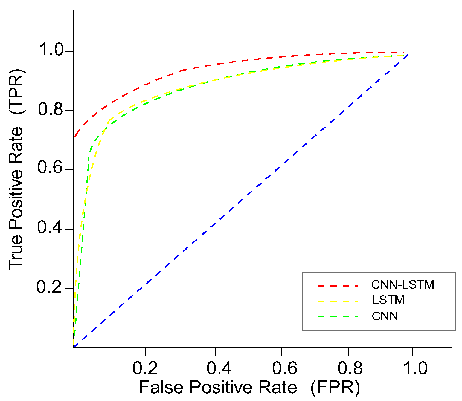
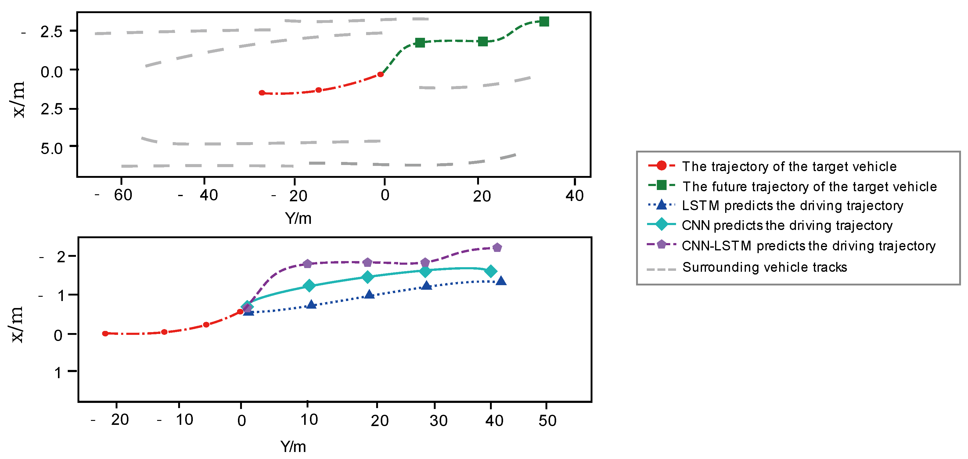
5.3. CNN-LSTM Trajectory Prediction Model Evaluation

A comprehensive evaluation of the model is performed using the receiver operating characteristic (ROC) curve, which illustrates the model’s performance by showing the true positive rate (TPR) and the false positive rate (FPR) at various classification thresholds. This approach enables a comprehensive assessment and comparison of the performance of the CNN-LSTM model with that of the standalone CNN and LSTM models. The ROC curve provides a comparison of the performance differences between models, and the area under the ROC curve (AUC) is calculated to quantify the model’s performance. The closer the AUC value is to 1, the better the model’s performance is.

The top-left corner represents the optimal point (Figure 6). The proposed CNN-LSTM model is closer to this point, indicating that it has a better generalization performance than the standalone CNN and LSTM models. Additionally, the AUC values calculated from the ROC curves in Figure 6 are 0.9854 for the CNN-LSTM model, 0.9478 for the CNN model, and 0.9351 for the LSTM model. Therefore, the CNN-LSTM model outperforms both the CNN and LSTM models.

The proposed CNN-LSTM model hierarchically extracts interactions, making it superior to individual CNN and LSTM models. Figure 7 compares the trajectory prediction results of the models. The scenario shows that changing to the left lane is a reasonable choice: in the current lane, the lead vehicle is decelerating; in the right lane, adjacent vehicles are moving faster than the target vehicle, providing no incentive to change lanes; and, in the left lane, adjacent vehicles are moving slower, with a safe distance sufficient for a lane change. While the LSTM and CNN models are almost incapable of predicting the future trajectory of the target vehicle, the CNN-LSTM model predicts the future trajectory more accurately.

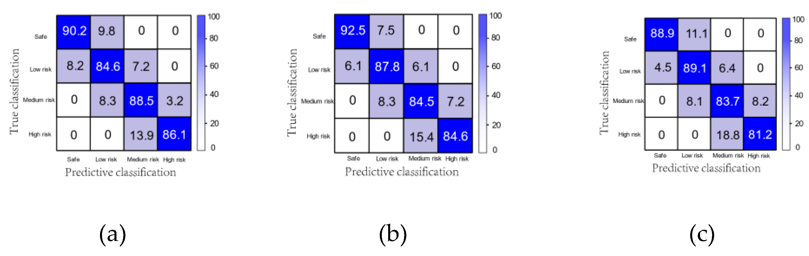
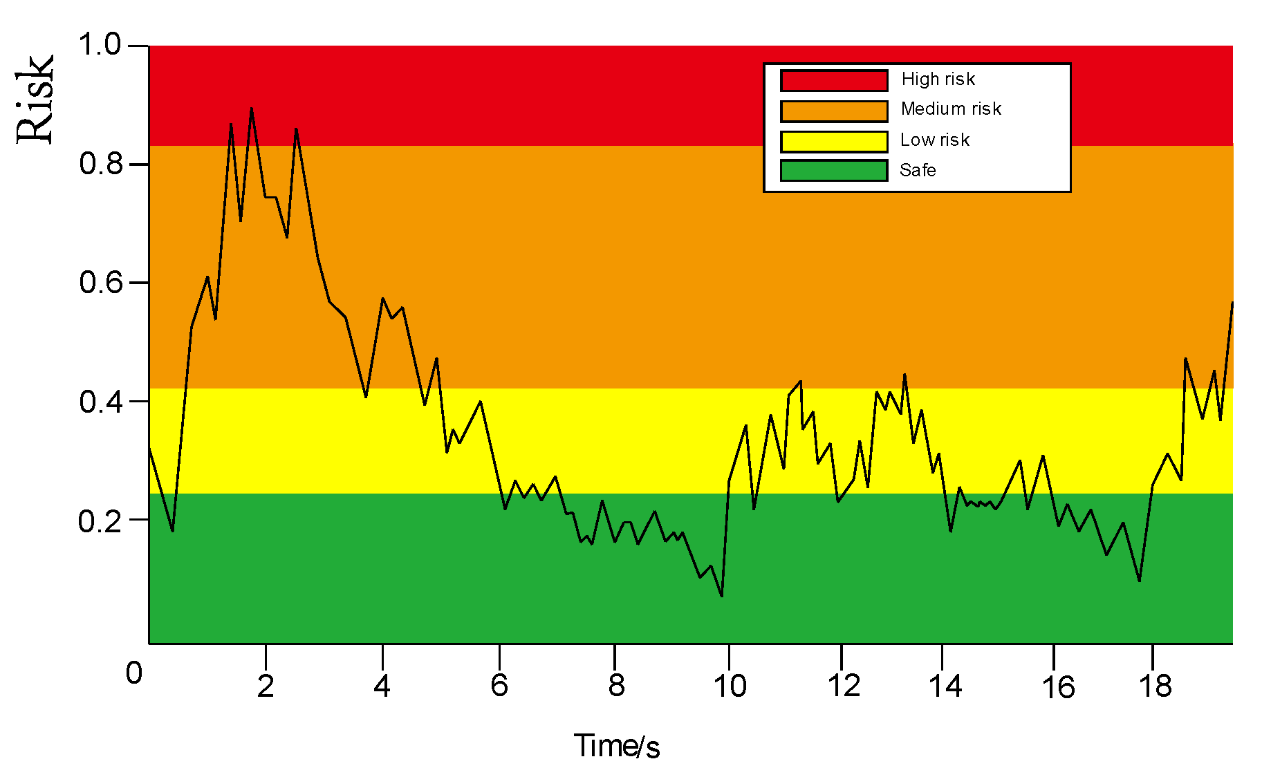
5.4. Risk Prediction Result Analysis

The model evaluation metrics can include Accuracy, Precision, Recall, and F1-score. By using Accuracy as the evaluation metric, the analysis can clearly highlight the differences between the CNN-LSTM model and the CNN and LSTM models. Figure 8 presents a comparative analysis of driving risk state predictions using different models. In Figure 8a, the proposed method achieves prediction accuracies of 84.6%, 88.5%, and 86.1% for low-risk, medium-risk, and high-risk scenarios, respectively. The CNN and LSTM models perform better than the CNN-LSTM model in predicting low-risk scenarios. However, for the target vehicle, it is preferable to predict low risk as medium or high risk to issue a warning, rather than mistakenly classifying medium or high risk as low risk. According to the results in Figure 8, the selected model achieves prediction accuracies of over 86% for both medium-risk and high-risk states.

To further demonstrate the predictive accuracy of the model regarding driving risks, the driving data from the dataset were used to illustrate the process of predicting changes in driving risk (Figure 9). The prediction model is quite sensitive to changes in risk, capable of capturing trends and patterns in risk variation. This demonstrates the model’s high accuracy and effectiveness in predicting driving risks.

6. Conclusions and Outlook

(1)

This study proposes an innovative CNN-LSTM deep-learning model that effectively predicts the future driving trajectories of target vehicles by integrating the characteristics of the CNN and LSTM. The model not only considers the dynamic interactions between vehicles but also incorporates multiple risk factors, such as the collision probability and severity, forming a comprehensive system for risk quantification and classification. By precisely categorizing different levels of risk, this model offers more accurate guidance for traffic management and safety interventions, contributing to a safer environment for autonomous driving.

(2)

The study utilizes the High-D dataset, which provides extensive real-world traffic scene data. Leveraging this dataset, the model accurately derives the target vehicle’s speed and acceleration based on the displacement and time changes between points along the predicted trajectory. This dynamic predictive capability enhances the model’s sensitivity to potential risks, achieving prediction accuracies exceeding 86% for moderate- to high-risk scenarios. Such a high accuracy and effectiveness offer crucial support for the safe operation of connected autonomous vehicles in complex traffic environments, while also improving the scientific rigor and reliability of overall traffic safety management.

(3)

There are still some limitations in the current study. In the future, the model will be expanded to incorporate references to hybrid integrated models in autonomous driving environments. Additionally, the effectiveness of the model in more complex traffic conditions, its applicability to other datasets, and its performance in environments such as highways will be explored to further enhance the driving safety of connected autonomous vehicles.

References

1. Kim, J.H.; Kum, D.S. Threat prediction algorithm based on local path candidates and surrounding vehicle trajectory predictions for automated driving vehicles. In Proceedings of the 2015 IEEE Intelligent Vehicles Symposium (IV), Seoul, Republic of Korea, 28 June–1 July 2015; pp. 1220–1225. [Google Scholar] [CrossRef]
2. Noh, S. Decision-making framework for autonomous driving at road intersections: Safeguarding against collision, overly conservative behavior, and violation vehicles. IEEE Trans. Ind. Electron. 2018, 66, 3275–3286. [Google Scholar] [CrossRef]
3. Li, G.; Yang, Y.; Zhang, T.; Qu, X.; Cao, D.; Cheng, B.; Li, K. Risk assessment based collision avoidance decision-making for autonomous vehicles in multi-scenarios. Transp. Res. Part C Emerg. Technol. 2021, 122, 102820. [Google Scholar] [CrossRef]
4. Zheng, X.; Jiang, J.; Huang, H.; Wang, J.; Xu, Q.; Zhang, Q. Novel quantitative approach for assessing driving risks and simulation study of its prevention and control strategies. J. Mech. Eng. 2024, 60, 207–221. [Google Scholar]
5. Xu, P.; Ruan, W.; Huang, X. Towards the quantification of safety risks in deep neural networks. arXiv 2020, arXiv:2009.06114. [Google Scholar]
6. Wang, C.; Liu, L.; Xu, C.; Lv, W. Predicting future driving risk of crash-involved drivers based on a systematic machine learning framework. Int. J. Environ. Res. Public Health 2019, 16, 334. [Google Scholar] [CrossRef] [PubMed]
7. Moon, S.; Koo, S.; Lim, Y.; Joo, H. Routing control optimization for autonomous vehicles in mixed traffic flow based on deep reinforcement learning. Appl. Sci. 2024, 14, 2214. [Google Scholar] [CrossRef]
8. Kong, D.; Wang, M.; Zhang, K.; Sun, L.; Wang, Q.; Zhang, X. Exploring HDV Driver-CAV interaction in mixed traffic: A Two-Step method integrating latent profile analysis and multinomial logit model. Appl. Sci. 2024, 14, 1768. [Google Scholar] [CrossRef]
9. Qu, D.; Meng, Y.; Wang, T.; Song, H.; Chen, Y. Car-following model and safety characteristics of connected autonomous vehicles based on molecular force field. J. Transp. Syst. Eng. Inf. Technol. 2023, 23, 33–41. [Google Scholar]
10. Johnsson, C.; Laureshyn, A.; De Ceunynck, T. In search of surrogate safety indicators for vulnerable road users: A review of surrogate safety indicators. Transp. Rev. 2018, 38, 765–785. [Google Scholar] [CrossRef]
11. Vogel, K. A comparison of headway and time to collision as safety indicators. Accid. Anal. Prev. 2023, 35, 427–433. [Google Scholar] [CrossRef] [PubMed]
12. Ozbay, K.; Yang, H.; Bartin, B.; Mudigonda, S. Derivation and validation of new simulation-based surrogate safety measure. Transp. Res. Rec. 2008, 2083, 105–113. [Google Scholar] [CrossRef]
13. Yang, H. Simulation-Based Evaluation of Traffic Safety Performance Using Surrogate Safety Measures. Ph.D. Thesis, Rutgers The State University of New Jersey, School of Graduate Studies, New Brunswick, NJ, USA, 2012. [Google Scholar]
14. Mahajan, V.; Katrakazas, C.; Antoniou, C. Crash risk estimation due to lane changing: A data-driven approach using naturalistic data. IEEE Trans. Intell. Transp. Syst. 2020, 23, 3756–3765. [Google Scholar] [CrossRef]
15. Rosen, E.; Stigson, H.; Sander, U. Literature review of pedestrian fatality risk as a function of car impact speed. Accid. Anal. Prev. 2011, 43, 25–33. [Google Scholar] [CrossRef] [PubMed]
Figure 1. CNN-LSTM framework.
Applsci 14 11204 g001
Figure 2. Historical trajectory representation diagram.
Applsci 14 11204 g002
Figure 3. Future trajectory car-following diagram.
Applsci 14 11204 g003
Figure 4. Future trajectory lane-change diagram.
Applsci 14 11204 g004
Figure 5. Collision probability and possibility in different scenarios: (a) low speed and long distance; (b) low speed and short distance; (c) high speed and long distance; and (d) high speed and short distance.
Applsci 14 11204 g005
Figure 6. ROC comparison curve.
Applsci 14 11204 g006
Figure 7. Trajectory prediction comparison.
Applsci 14 11204 g007
Figure 8. Driving risk state prediction comparison: (a) CNN-LSTM; (b) CNN; and (c) LSTM.
Applsci 14 11204 g008
Figure 9. Illustration of driving risk variation.
Applsci 14 11204 g009