An Enhanced Deep Q Network Algorithm for Localized Obstacle Avoidance in Indoor Robot Path Planning

Abstract

Path planning is a key task in mobile robots, and the application of Deep Q Network (DQN) algorithm for mobile robot path planning has become a hotspot and challenge in current research. In order to solve the obstacle avoidance limitations faced by the DQN algorithm in indoor robot path planning, this paper proposes a solution based on an improved DQN algorithm. In view of the low learning efficiency of the DQN algorithm, the Duel DQN structure is introduced to enhance the performance and combined with a Prioritized Experience Replay (PER) mechanism to ensure the stability of the robot during the learning process. In addition, the idea of Munchausen Deep Q Network (M-DQN) is incorporated to guide the robot to learn the optimal policy more effectively. Based on the above improvements, the PER-D2MQN algorithm is proposed in this paper. In order to validate the effectiveness of the proposed algorithm, we conducted multidimensional simulation comparison experiments of the PER-D2MQN algorithm with DQN, Duel DQN, and the existing methodology PMR-DQN in the Gazebo simulation environment and examined the cumulative and average rewards for reaching the goal point, the number of convergent execution steps, and the time consumed by the robot in reaching the goal point. The simulation results show that the PER-D2MQN algorithm obtains the highest reward in both static and complex environments, exhibits the best convergence, and finds the goal point with the lowest average number of steps and the shortest elapsed time.

1. Introduction

As artificial intelligence and robotics rapidly advance, mobile robots are being increasingly utilized in sectors such as industrial manufacturing, medical science, social science, agriculture, education, games, and space research [1]. Autonomous navigation [2] technology, as the core of mobile robots for achieving autonomous mobility and intelligent decision-making, directly affects the work efficiency and adaptability of robots. Autonomous navigation requires the robot to not only avoid obstacles in known or unknown environments, but also dynamically adjust the path to adapt to environmental changes, thereby ensuring efficient completion and safety of the task. Effective autonomous navigation technology can not only improve the autonomy of robot task execution, but also reduce human intervention and reduce operating costs.

It means that the mobile robot autonomously designs the path from the starting point to the end point, with the shortest distance, the shortest time consumed, and the safest and most collision-free path [3]. Path planning can be categorized into offline learning and online learning methods [4]. Offline learning refers to the process of pre-training a model before the robot executes its tasks, and then applying this model during actual operation. The advantage of this approach is that it allows for extensive optimization and adjustment using large amounts of data during the training phase. Typical offline learning path planning algorithms include the A* algorithm and Dijkstra’s algorithm, among others [5]. Online learning, on the other hand, involves real-time learning and updating of the model as the robot performs its tasks. The advantage of online learning lies in its ability to dynamically adapt to environmental changes, thereby enhancing the flexibility and robustness of path planning. Typical online learning path planning algorithms include the Artificial Potential Field (APF) [6] and Deep Reinforcement Learning (DRL) [7]. For instance, DQN approximates the Q-value function using a Deep Neural Network, enabling effective online path planning in high-dimensional state spaces [8].

Despite the significant progress in the application of DRL in path planning [9], such as DQN, Double DQN [10] and Duel DQN [11], the existing methods still face some problems. First, the traditional DQN converges slowly in high-dimensional state space, which makes it difficult to adapt to the dynamic environment quickly. Second, the stochastic experience playback mechanism is difficult to effectively utilize the key experience, which affects the quality of strategy learning. Moreover, in complex environments, the reward function has limited guidance for strategy learning, which easily leads to instability.

Aiming at the above problems, this paper proposes an improved deep reinforcement learning algorithm, **PER-D2MQN**, whose innovativeness is mainly reflected in the following aspects:

(1)

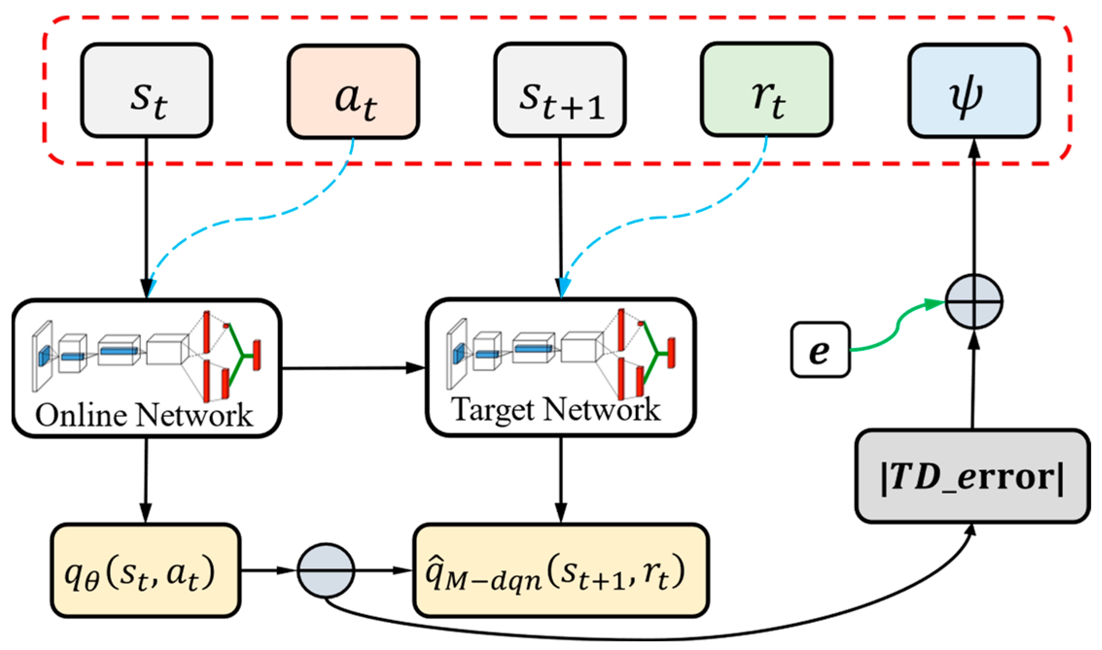
The PER mechanism is introduced to optimize the sample selection strategy, prioritize the use of key experiences, and accelerate the learning process;

(2)

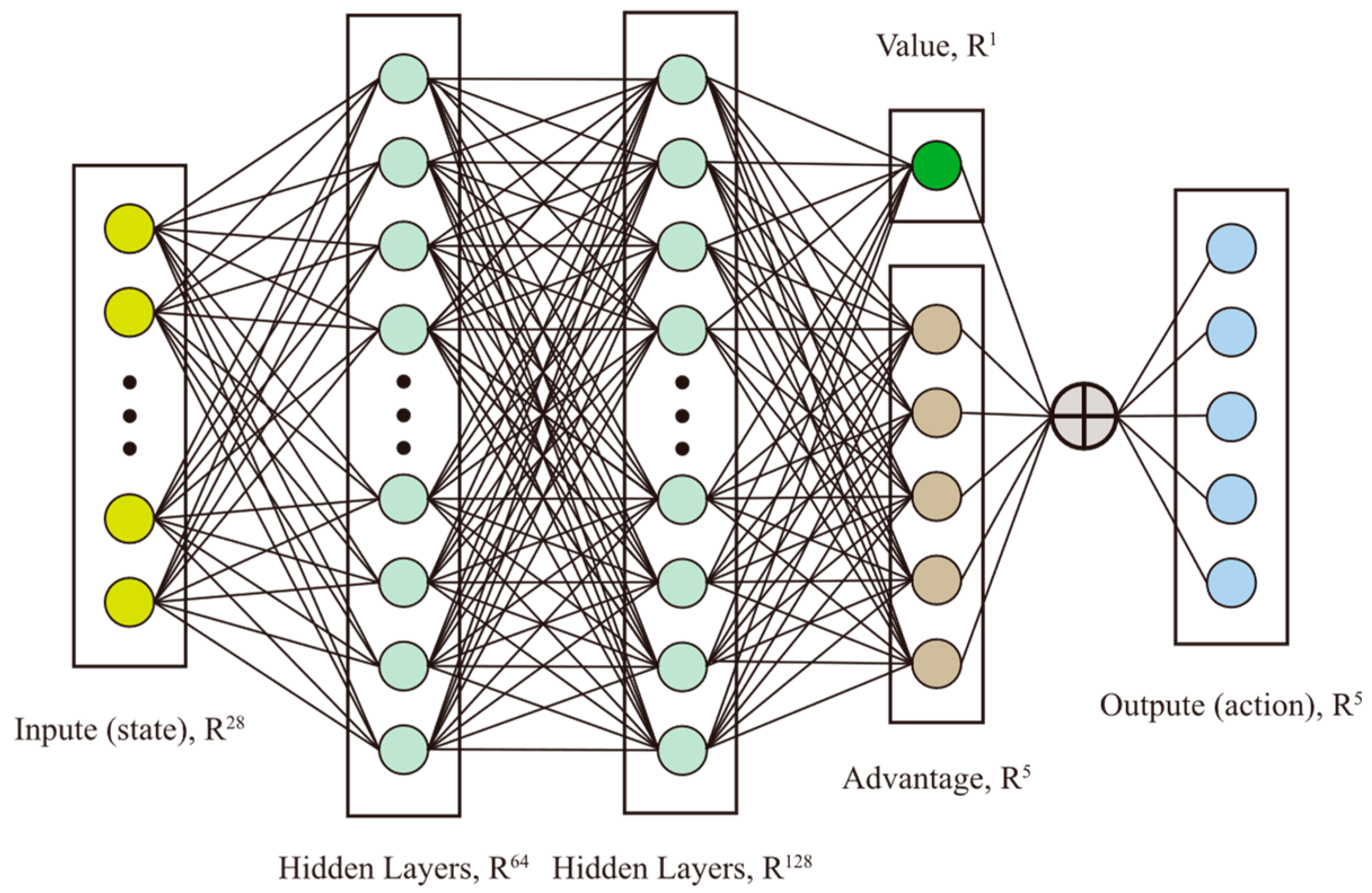
Adopting the Duel DQN structure to improve strategy stability and learning efficiency by decomposing the value function and advantage function;

(3)

Drawing on Munchausen’s idea of reinforcement learning, a regularized “logarithmic strategy” is added to enhance the robustness of the reward signal and further improve the performance and stability of the algorithm.

The subsequent structure of this article is as follows: Section 2 introduces “Related work” and demonstrates the application of DQN algorithm in path planning; Section 3 introduces “Implementation based on PER-D2MQN algorithm”; Section 4 introduces “Environment design”, including action design of turtlebot3 robot, state design and reward function; Section 5 introduces “Experimental analysis”, which proves the superiority of the PER-D2MQN algorithm; and Section 6 is “Conclusion”, which explains the shortcomings of this study and future work.

2. Related Work

In recent years, RL has emerged as a research focus in the field of online path planning due to its immunity to environmental mutations and dynamic obstacles [4]. Reference [12] has shown this by simulating two scenarios: the first scenario where the map changes while the intelligent body is moving, and the second scenario where dynamic obstacles appear on a static map. It is demonstrated that real-time Q Learning can be used for mobile robot path planning and dynamic obstacle avoidance in various environments. Reference [13] introduced priority weights into Q Learning to improve the value assessment of the algorithm when solving practical problems. The improved algorithm significantly improved the average speed and accuracy and was able to find better paths in dynamic environments. Reference [14] proposed an Optimized Q Learning (O_QL) algorithm to address the problems of slow convergence and easy trapping in local optimal solutions of the Q Learning algorithm. O_QL introduced a new Q table initialization method and adopted a new action selection strategy that combines the ε-greedy and Boltzmann strategies. In order to avoid sparse rewards, it borrowed the Gaussian idea to use a continuous reward function. Reference [15] adopts the concept of partially guided Q Learning and uses the APF method to improve the classical Q Learning method. The proposed QAPF algorithm overcomes the shortcomings of classical Q Learning such as slow learning speed, long learning time and slow convergence. The above reference has made corresponding improvements to the Q Learning algorithm by iteratively updating the Q table, exploring strategies, reward functions, and learning rates, significantly improving the convergence efficiency and learning speed of the algorithm, enabling it to cope with general unknown dynamic environments, but it cannot solve the “dimensionality curse” problem. Q Learning performs well in discrete state and action spaces, but for continuous spaces, discretization is required, which may introduce approximation errors.

In 2015, in order to solve the memory overflow problem caused by large amounts of data or upcoming continuous actions in high-dimensional environments, DeepMind proposed the DQN [8] algorithm in Nature, which combines neural networks with Q Learning. The authors of [16] used the PER mechanism in the DQN algorithm. By determining the importance of experience based on TD error, high-priority experience is replayed more frequently, and random priority and importance sampling weight corrections are introduced to ensure sample diversity and unbiased updates. These improvements enable the DQN algorithm to use experience data more effectively, accelerate learning without increasing the number of interactions with the environment, and significantly improve the quality of the strategy, especially in Atari game tests. The authors of [17] introduced maximum entropy into RL, making the strategy more random when choosing actions. The introduction of this entropy regularization increases the diversity of exploration, thereby exploring the environment more effectively in the early stages, and ultimately speeding up the entire learning process. The authors of [18] maximized the expected return and the entropy of the final policy by adding a scaled “log-policy” to the instant reward based on maximum entropy RL. This approach makes the M-DQN algorithm the first algorithm to outperform distributional RL without using distributional RL [19].

Reference [20] drew on the network branching structure of Duel DQN to design a dual-branch network that decouples obstacle avoidance and navigation tasks. It also adopted an “expert experience” approach to improve random exploration and designed a unique reward function mechanism. Through both simulation and real-world experiments, the algorithm’s advantages in terms of convergence and stability were demonstrated. The authors of references [21,22] both adopted the Double DQN approach to alleviate the overestimation issue in DQN. Reference [21] cleverly combines the RRT strategy to address the challenge of Double DQN failing to learn new experiences, while also integrating A* algorithm ideas into the reward mechanism to tackle the model convergence issue. Reference [22] combines Hindsight Experience Replay with Double DQN to mitigate the negative impact of sparse rewards. Both studies demonstrated the effectiveness of their algorithms in a 2D grid map. However, it remains uncertain whether these algorithms can be effectively applied in unknown environments.

References [23,24,25,26,27] combine DQN with APF, utilizing the obstacle avoidance capability of APF and the learning ability of DQN to improve the path planning effect of mobile robots or drones in complex environments, thereby improving efficiency and success rate and addressing the shortcomings of traditional methods in complex dynamic environments. Ref. [23] proposed DM-DQN, which combines the dueling network and Munchausen strategy, and designed a reward function based on APF. Reference [24] uses APF as prior knowledge, introduces the SA-ε-greedy algorithm to adaptively adjust the random exploration frequency, and uses a multi-output neural network and B-spline algorithm. Reference [25] optimized the path planning of UAVs in urban environments by improving the action space and reward mechanism. Reference [26] improved the robot’s navigation ability in static and dynamic obstacle environments by introducing APF into the reward function. At the same time, the knowledge transfer method was used to migrate the training model in a simple environment to a complex environment, which accelerated training and convergence. These algorithms solve the shortcomings of traditional methods in complex environments by combining the obstacle avoidance of APF and the learning ability of DQN. However, these methods still face generalization and stability issues in extremely complex and dynamic environments, which require further research and optimization.

The research in references [28,29,30,31] all focuses on the path planning problem of UAVs in three-dimensional environments, and is committed to optimizing the autonomous navigation and obstacle avoidance capabilities of UAVs in complex terrain and obstacle environments. Ref. [28] proposed a Retrospective-Based Deep Q Learning (R-BDQL) method, which reduces the overestimation problem in Q-value estimation by introducing a retrospective mechanism. For extremely complex environments, it may take a lot of time to optimize the algorithm, and in certain cases, overfitting problems may occur. Ref. [30] Combining the heuristic function with the maximum average reward experience replay mechanism improves sample utilization and algorithm convergence speed. However, in large-scale dynamic environments, the heuristic information may not be accurate enough, affecting the path planning effect. Ref. [31] introduced a Memory-Enhanced (ME) mechanism combined with the Duel DQN to effectively reduce collision events in early training. However, in extremely complex or dynamic environments, the ME may lead to low memory utilization and fail to adapt to environmental changes.

To sum up, DRL is often used to address local path planning and real-time obstacle avoidance challenges. According to its implementation method, RL can be divided into two categories: model-based and model-free [32,33]. Model-based methods, such as Q Learning, rely on explicit environmental models, such as state-action tables. Model-free methods do not require detailed information about the environment and learn the best strategy through exploration. These model-free methods can be further divided into value-based learning algorithms and policy-based learning algorithms. Value-based methods train agents by evaluating the results of performing specific actions in specific states, while policy-based methods directly construct a mapping strategy from state to action [34,35,36]. DQN used in this study belongs to the category of value-based model-free algorithms that guide the decision-making process of agent by roughly modeling the unknown environment.

3. Implementation Based on PER-D2MQN Algorithm

In this section, we will describe in detail the implementation process of the PER-D2MQN algorithm framework. First, we will introduce the theoretical basis based on the Markov decision process, as well as the principle and implementation of the adopted Duel DQN structure. Next, we will explain the working principle and update process of the Prioritized Experience Replay Buffer (PERB) and finally discuss the main improvements of the M-DQN algorithm to the DQN regression target. Figure 1 shows the overall process of the PER-D2MQN algorithm to implement local path planning in the Gazebo environment. Specifically, the robot selects an action $a_t$ through the $\epsilon -greedy$ strategy and acts on the environment, so that the environment changes from the current state $s_t$ to the next state $s_{t+1}$ and, at the same time, gives feedback to the robot with an instant reward $r_t$, and then stores $s_t,a_t,r_t,s_{t+1}$ as experience samples in the replay buffer. During the network training process, the number of samples is selected by the empirical priority weight $\psi$, and the online network parameters are copied to the target network according to the predetermined rule. Then, the loss function is calculated using the current network and the target network, and the parameters are updated through back propagation.

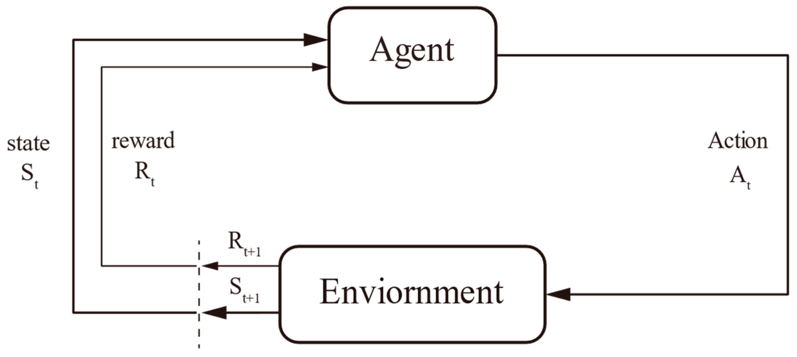
3.1. Theoretical Foundation

Markov decision process (MDP) is a mathematical framework for RL problems. It provides a structured method to describe the environment in RL and defines the rules for the agent to make decisions in the environment, as shown in Figure 2. Although MDP is a widely used model for decision-making problems, in the real world, we usually cannot fully observe the entire state of the environment. For example, a robot’s 2D LIDAR sensor can only provide limited distance information and cannot fully describe its environment. In this case, using POMDP [33,37] to define the problem is more in line with the actual situation. Specifically, POMDP can be described as a tuple $<S.A.T.R.\gamma .\Omega .O>$. The elements of the tuple are interpreted as follows:

$S$: All states of the environment; $\forall s\in S$

$A$: All actions the agent can take; $\forall a\in A$

$T$:$S\times A\to \pi \left(S\right)$ is the state transition function, which gives the probability that the agent takes action $a$ in a certain state and ends up in state $s‘$; $T\left(a,s,s‘\right)=\pi \left(s‘|s,a\right),\forall s,s‘\in S and \forall a\in A$

$R$:$S\times A\to \mathbb{R}$ is the instant reward;

$\gamma \in \left[\mathrm{0,1}\right]$ is the discount factor;

$\Omega$ is all the information that the agent may observe;

$O$: $S\times A\to \pi \left(\Omega \right)$ is an observation function that gives the probability of observing o if the agent takes action $a$ and ends up in state $s‘$; $O(s‘,a,o)=\pi \left(o\right|s‘,a),\forall s,s‘\in S \mathrm{a}\mathrm{n}\mathrm{d} \forall a\in A \mathrm{a}\mathrm{n}\mathrm{d} \forall o\in \mathsf{\Omega }$.

As a typical RL algorithm, the Q Learning algorithm can iteratively estimate the optimal action value function $q_{\mathrm{*}}(\mathrm{s},\mathrm{a})$ by updating Equation (1):

$$q(s_t{a}_t)\leftarrow q(s_t,a_t)+\alpha [r_t+\gamma \underset{a‘}{ \max }{q}_{\mathrm{*}}(s_{t+1},a‘)-q(s_t,a_t)]$$

(1)

where $q(s_t,a_t)$ denotes the current estimated value of taking action $a_t$ in state $s_t$; $s_t$ denotes the state of the intelligent body at time step $t$; $a_t$ denotes the action taken by the intelligent body at time step $t$; $r_t$ denotes the immediate reward obtained by the agent at time step $t$; $s_{t+1}$ denotes the new agent at time step $t+1$ state; $\alpha$ is the learning rate, which controls the learning speed; $\gamma$ is the discount factor, which weighs the importance of immediate and future rewards. In practice, the optimal value $q$ function $q_{\mathrm{*}}$ is usually unknown, and we can only use the value function $q(s_t,a_t)$ of the current strategy in place of the value function $q_{*}$ of the optimal strategy. This process is often called bootstrapping. In short, bootstrapping means updating the current estimate $q(s_t,a_t)$ to a new estimate $q(s_{t+1},a‘)$, i.e., improving one’s own estimate by using the current estimate.

Q Learning algorithms are inefficient and difficult to scale when faced with complex and multi-state real-life problems. DRL provides an effective way to solve this problem under the POMDP framework: DQN, which approximates the Q value function by training an Artificial Neural Network (ANN). The trained ANN model serves as a function approximator for the Q function, capable of managing complex state spaces. The agent chooses actions based on observation vectors from the environment, utilizing a model with a Deep Neural Network (DNN) architecture.

3.2. Duel DQN Structure Model

For the bootstrap-based DQN algorithm, the estimation of the state value is crucial for each state. Duel DQN introduces a competitive network structure to update the values of all actions at the same time when the Q value is updated. More precisely, the Q value can be split into two components: the state value and the action advantage, as shown in Equation (2):

$$Q\left(s,a;\theta ,\alpha ,\beta \right)=V\left(s;\theta ,\beta \right)+A\left(s,a;\theta ,\alpha \right)$$

(2)

Centering is required due to the uncertainty in the advantage function $A\left(s,a;\theta ,\alpha \right)$ and the combination of the state value function $V\left(s;\theta ,\beta \right)$, which may lead to unstable Q-value estimates. The centering process ensures uniqueness and stability by subtracting the mean of the dominance function. The adjusted Q-value function is represented as shown in Equation (3):

$$Q\left(s,a;\theta ,\alpha ,\beta \right)=V\left(s;\theta ,\beta \right)+\left(A\left(s,a;\theta ,\alpha \right)-{\displaystyle \frac{1}{\left|A\right|}}\sum _{a‘}A\left(s,a‘;\theta ,\alpha \right)\right)$$

(3)

where $s$ represents the state, $a$ represents the action, $a$ and $\beta$ are the specific parameters of the advantage function $A\left(s,a;\theta ,\alpha \right)$ and the state value function $V\left(s;\theta ,\beta \right)$, respectively, $\theta$ is a shared network parameter, and $A$ is the size of the action space. The experiment in the reference [11] proved that this more frequent value updating method enhances the convergence speed and learning efficiency of DQN.

The Duel DQN structure used by the PER-D2MQN algorithm is shown in Figure 3, Its main structure comprises an input layer, three hidden layers, and an output layer. The input layer corresponds to 28 state sets, the first two hidden layers are fully connected layers, containing 64 and 128 units, respectively, and the third hidden layer is the main feature of the Duel DQN structure, which is divided into a value function consisting of one unit and an advantage function consisting of five units of action sets.

3.3. Prioritized Experience Replay Buffer

As one of the two major features of the DQN algorithm, the Experience Replay Buffer (ERB) is a storage device that stores experience data during the agent’s interaction with the environment. By randomly sampling small batches of experience from it, the time correlation is broken and the stability and efficiency of training are improved. The experience data set is continuously updated. When the buffer is full, the old experience is replaced so that the new and old data can be used together to train the model. However, the uniform random sampling of ERB may ignore some experiences that are more important to the learning process and fail to make full use of these key experiences to accelerate learning.

To solve the above shortcomings, the PER [16] was proposed. It considers the importance of empirical data through the TD error ${\delta }_i$, as shown in Equation (4):

$$\psi =\left|{\delta }_i\right|+e$$

(4)

$e$ is an extremely small positive constant used to prevent the priority from being 0. In order to perform weighted sampling according to priority, PER uses the proportional priority method. The probability $P\left(i\right)$ of experience i being sampled is defined as shown in Equation (5):

$$P\left(i\right)={\displaystyle \frac{p_i^{\alpha }}{{\sum }_k{p}_k^{\alpha }}}$$

(5)

where $\alpha$ is a hyperparameter that controls the degree of prioritization, reverting to uniform random sampling when $\alpha =0$, and sampling exactly according to priority when $\alpha =0$. In order to correct the bias caused by weighted sampling, importance sampling weights ${\omega }_i$ are introduced to adjust the gradient update of the loss function as in Equation (6):

$${\omega }_i={\left({\displaystyle \frac{1}{N}}·{\displaystyle \frac{1}{P\left(i\right)}}\right)}^{\beta }$$

(6)

$N$ is the total size of the experience pool, and $\beta$ is a hyperparameter used to balance the initial and later importance corrections, usually starting from a smaller value and increasing gradually, eventually approaching 1. The PERB used in this paper updates a tuple of experiences at moment t as shown in Figure 4.

3.4. PER-D2MQN

The bootstrap mechanism in RL based on time difference learning usually uses the estimated value of the current state to replace the true value of the next state. M-DQN introduces an additional guidance signal “log-policy”. If the optimal deterministic policy ${\pi }_{\mathrm{*}}$ is known, after the policy is “log” operated, the probability of selecting the optimal action is 0, and the probability of selecting the non-optimal action is $-\mathrm{\infty }$. Such a guidance signal is more advantageous in policy selection because it can effectively suppress the selection of non-optimal policies. However, the optimal policy ${\pi }_{\mathrm{*}}$ is usually unknown, so $\pi$ is used instead of ${\pi }_{\mathrm{*}}$ and the random policy is assumed to satisfy numerical stability.

The loss function of the DQN can be represented by ${\widehat{\mathbb{E}}}_B\left[{\left(q_{\theta }\right(s_t,a_t)-{\widehat{q}}_{dqn}(r_t,s_{t+1}\left)\right)}^2\right]$, where the regression target of DQN ${\widehat{q}}_{dqn}$ can be expressed as Equation (7):

$${\widehat{q}}_{dqn}\left(r_t,s_{t+1}\right)=r_t+\gamma \sum _{a‘\in A}{\pi }_{\overline{\theta }}\left(a‘|s_{t+1}\right)q_{\overline{\theta }}\left(s_{t+1},a‘\right) with {\pi }_{\overline{\theta }}\in \mathcal{G}\left(q_{\overline{\theta }}\right)$$

(7)

DQN can derive M-DQN by modifying the regression objective, but since M-DQN adopts a stochastic policy ($softmax$ policy, satisfying $\pi =sm(q)\iff \pi (a|s)={\displaystyle \frac{expq(s,a)}{{\sum }_{a‘}expq(s,a‘)}}$), whereas DQN computes a deterministic policy ($greedy$ policy, satisfying $\pi \left(a\right|s)=1 \mathrm{f}\mathrm{o}\mathrm{r} \mathrm{a} \in {argmax}_{\mathrm{a}‘}q(s,a‘)$ for $\pi \in \mathcal{G}\left(q\right)$). A simple solution is to maximize not only the return but also the entropy of the resulting strategy, i.e., to adopt the maximum entropy RL viewpoint by introducing the Soft Actor-Critic (SAC) [14] algorithm into the DQN to form the Soft-DQN (S-DQN), whose regression objective is represented by Equation (8):

$$\begin{array}{ll}{\widehat{q}}_{s-dqn}\left(r_t,s_{t+1}\right)=& r_t+\gamma {\displaystyle \sum _{a‘\in A}}{\pi }_{\overline{\theta }}\left(a‘|s_{t+1}\right)\\ & \left(q_{\overline{\theta }}\left(s_{t+1},a^{‘}\right)-\tau \ln {\pi }_{\overline{\theta }}\left(a^{‘}|s_{t+1}\right)\right) \mathrm{with} {\pi }_{\overline{\theta }}=sm(q_{\overline{\theta }}/\tau )\end{array}$$

(8)

where $\tau$ is the temperature coefficient scaling the entropy, $r_t$ is the instant reward, $\gamma$ is the discount factor, $a‘$ is the action at moment $t+1$, $s_{t+1}$ is the state at moment $t+1$, and $A$ denotes the action space. When $\mathit{limit}\tau \to 0$, S-DQN is denoted as DQN.

The regression target of M-DQN is to add scaled log-policy to the instant reward of S-DQN, i.e., $\alpha \tau \mathit{ln}{\pi }_{\overline{\theta }}\left(a_t|s_t\right)$. The specific expression is shown in Equation (9):

$$\begin{array}{ll}{\widehat{q}}_{M-dqn}\left(r_t,s_{t+1}\right)=& r_t+\alpha \tau \ln {\pi }_{\overline{\theta }}\left(a_t|s_t\right)+\gamma {\displaystyle \sum _{a‘\in A}}{\pi }_{\overline{\theta }}\left(a^{‘}|s_{t+1}\right)\\ & \left(q_{\overline{\theta }}\left(s_{t+1},a^{‘}\right)-\tau \ln {\pi }_{\overline{\theta }}\left(a‘|s_{t+1}\right)\right) \mathrm{with} {\pi }_{\overline{\theta }}=sm(q_{\overline{\theta }}/\tau )\end{array}$$

(9)

Setting $\alpha \in \left[\mathrm{0,1}\right]$ as the scaling factor and when $\alpha =0$, ${\widehat{q}}_{M-dqn}={\widehat{q}}_{s-dqn}$. Then, the loss function of M-DQN can be represented as ${\widehat{\mathbb{E}}}_B\left[{\left(q_{\theta }\right(s_t,a_t)-{\widehat{q}}_{M-dqn}(r_t,s_{t+1}\left)\right)}^2\right]$. Experiments in the reference [15] demonstrate that M-DQN outperforms any of the distributed RL algorithms on Atari games and show that M-DQN is suitable for any TD-based RL.

PER-D2MQN firstly adopts the PER mechanism to assign priorities to each experience, samples are weighted according to the priorities, and the TD errors of the experiences are used to update the priorities; then, the network structure of Duel DQN is utilized to improve the computational efficiency of Q-values. Finally, M-DQN is introduced by adding a “log-policy” term of the probability of the strategy to the instant reward, i.e., by replacing $r_t+\alpha \tau \mathit{ln}{\pi }_{\overline{\theta }}\left(a_t|s_t\right)$ instead of $r_t$ to strengthen the signal and optimize the learning process. Part of the pseudo-code for the PER-D2MQN algorithm is provided in Algorithm 1.

Algorithm 1: PER-D2MQN Algorithm

Input:$\mathrm{Prioritized} \mathrm{Experience} \mathrm{Replay} \mathrm{Buffer} \left(\mathit{P}\right)$  Output:$\mathrm{Trained} \mathrm{network} \mathrm{with} \mathrm{parameters} \mathsf{\theta }$ 1  Initialize $\mathit{P}$ 2  Initialize online network and target network with random weights and biases 3  for episode $=$ 1 to E do 4       Initialize state $s$ (Reset Environment) 5       for t $=$ 1 to episode_step do 6            Observe state $s$ and input state $s$ into online network 7            Select action $a$ using $\epsilon -greedy$ 8            Execute action $a$ in the environment, get $r$, $s‘$, and flag 9            Store experience ($s, a, r, s‘, done$) into $\mathit{P}$ with maximum priority $\mathsf{\psi }$ of $\mathit{P}$ 10          if size of $\mathit{P}$ $>$ batch _size then 11                Sample batch from $P$ based on priority weights $\mathsf{\omega }$ 12                for each ($s_i, a_i, r_i, s_i^{‘}, {done}_i$) in batch do 13                       Compute $Q(s_i, a_i)$; 14                       Compute Munchausen log policy term: $\log \pi \left(a_i\right| s_i)=Q(s_i‘ a_i)- \log {\sum }_b\mathrm{e}\mathrm{x}\mathrm{p}\left(Q\right(s_i,b\left)\right)$ 15                       Compute Munchausen reward: $r_i^{‘}=r_i+\alpha \tau \log \pi \left(a_i\right| s_i)$ 16                       Compute target: $y_i=r_i‘+\gamma (1-{done}_i){\sum }_a‘\pi \left(a‘\right| s_i‘)(Q‘\left(s_i‘, a‘\right)- \tau \log \pi \left(a‘\right| s_i‘)$ 17                       Compute target: ${\psi }_i=\left|y_i-Q\left(s_i, a_i;\theta \right)\right|+e$ 18                Compute loss: $L={\displaystyle \frac{1}{N}}{\sum }_i{\omega }_i{{\psi }_i}^2$ 19                Update priorities in $\mathit{P}$ 20                Gradient descent on loss 21        if global_step % target update $==$ 0 then 22              Update target network ${\mathsf{\theta }}^{-}=\mathsf{\theta }$ 23       if done then 24              Break 25        Increment global_step  26   if $\epsilon >{\epsilon }_{min}$ then  27      ${ \epsilon }^{*}={\epsilon }_{decay}$

4. Environment Design

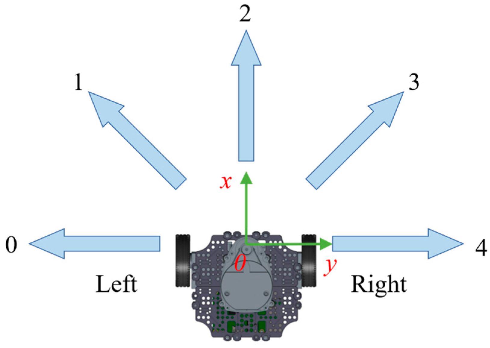
4.1. Action Design of Turtlebot3 Robot

In this study, we use the DRL algorithm to control the angular and linear velocities of the turtlebot3 robot, thus allowing the robot to perform the five-direction moving action shown in Figure 5, in which the linear velocity of the mobile robot is fixed at 0.15 m/s and the angular velocities are set to five values shown in

Table 1. Turtlebot3 robot movements and corresponding angular velocity.

Action	0	1	2	3	4
Angular Velocity $\mathrm{rad}/\mathrm{s}$	−1.5	−0.75	0	0.75	1.5

depending on the direction of motion of the realized robot.

4.2. State Design of Turtlebot3 Robot

The Turtlebot3 robot acquires the environment information through LIDAR, and the purpose of the PER-D2MQN Agent is to allow the robot to navigate around obstacles and reach the goal point. The coordinates of the robot’s position relative to the target and obstacles change in real time with uncertainties. Figure 6 shows the spatial state of the Turtlebot3 robot for local path planning in this study, which mainly includes the robot’s start position $(x_r,y_r)$, the Euclidean distance $d_g$ between the robot and the target position $(x_g,y_g)$ and the heading angle ${\theta }_g$ between the robot heading and $d_g$. The robot fires 24 laser rays through LIDAR. The minimum distance $d_o$ of the nearby obstacle is acquired by $LSD\left(24\right)$ and the index n when $d_o$ is detected. The state set $s_t$ is specifically represented as shown in Equation (10).

$$s_t=LDS\left(24\right)+d_g+{\theta }_g+d_o+n$$

(10)

4.3. Reward Function

The reward function is crucial in RL environments, and directly guides the behavior and decision-making process of an intelligent body by defining the rules of reward and punishment. A well-designed reward function can accelerate the learning process, motivate the intelligent body to effectively explore and find the optimal strategy, while avoiding getting stuck in local optima, thus significantly improving the performance and adaptability of the intelligent body in complex environments.

In this study, a variety of factors such as robot orientation, distance to target, distance to obstacles, and task completion status are considered to design the reward function in order to effectively guide the robot’s navigation and decision-making in the Gazebo environment. The specific design is as follows.

By evaluating the difference between the robot’s current facing direction and the target direction, the facing reward is designed by encouraging the robot to progress toward the target direction. This is shown in Equation (11):

$$r_{yaw}=1-4\left|0.5-\left(0.25+0.5\times \left({\displaystyle \frac{\theta \mathrm{\%}\left(2\pi \right)}{\pi }}\right)\right)\right|$$

(11)

The distance reward is designed to encourage the robot to approach the target position by calculating the distance ratio between the robot’s current position and the target position. The specific design is shown in Equation (12):

$$r_d=2^{{\displaystyle \frac{d_c}{d_g}}}$$

(12)

where ${\mathrm{d}}_{\mathrm{c}}$ represents the distance between the robot’s current position and the target point, and $d_g$ denotes the distance from the start point of the robot to the target point.

The obstacle reward is designed to ensure that the robot can effectively avoid obstacles during the path planning process. The specific design is shown in Equation (13):

$$r_{ob}=\left\{\begin{array}{l}-5,if d_o<0.5\\ 0,others\end{array}\right.$$

(13)

where $d_o$ denotes the minimum distance of nearby obstacles acquired by the robot through the laser sensor. Based on the above reward design, the total reward function can then be formulated as in Equation (14):

$$r=\left(r_{yaw}\left[action\right]\times 5\times r_d\right)+r_{ob}$$

(14)

Then, the overall reward function for the robot to realize obstacle avoidance and path planning in the Gazebo environment can be designed as in Equation (15):

$$R=\left\{\begin{array}{cc}-500,\hfill & \hfill if Goal(d_g<r_g)\hfill \\ 1000,\hfill & \hfill if Collision(d_{ob}<r_{ob})\hfill \\ r,\hfill & \hfill others\hfill \end{array}\right.$$

(15)

4.4. Exploration Strategy

The $\epsilon -greedy$ strategy used in this paper is a method for balanced exploration and exploitation with the aim of learning the best strategy in an unknown environment. The strategy controls the choice behavior of an intelligent body when taking action by introducing a parameter called $\epsilon \in \left(\mathrm{0,1}\right)$. Specifically, under the $\epsilon -greedy$ strategy, the intelligent body randomly selects an action with a probability of $\mathsf{ϵ}$, and selects the currently known optimal action with a probability of $1-\epsilon$. This strategy ensures that the agent has a certain chance to try the unknown action space in order to discover a potentially more optimal strategy, thus improving the efficiency and effectiveness of learning. It is expressed as Equation (16):

$$a=\left\{\begin{array}{c}random action, p<\epsilon \\ \underset{a‘\in A}{\mathit{arg}\mathit{max}}Q\left(s,a‘\right), p\ge \epsilon \end{array}\right.$$

(16)

where $p\in \left(\mathrm{0,1}\right)$ is denoted as the random number generated when the intelligent body learns.

4.5. Assumptions

The robot is equipped with LiDAR, which is capable of detecting the distance and direction of surrounding obstacles with a certain level of measurement accuracy and noise level. The motion of the robot is based on non-complete constraints with differential drive mode. Velocity constraints are as follows: linear velocity $v\in [0,0.35 \mathrm{m}/\mathrm{s}]$ and angular velocity $\omega \in [-1.5,1.5 \mathrm{rad}/\mathrm{s}]$. The robot cannot exceed the designed maximum steering angle range at any moment.

5. Experimental Analysis

5.1. Experimental Platform and Parameter Setting

The experimental research in this paper was based on the Ubuntu 20.04 operating system with a hardware configuration of 16GB RAM, 100 GB hard disk, Nvidia 4060 graphics card, and a 12th Gen Intel^® Core™ i5-12400F 12-core processor (The processor, manufactured by Intel Corporation, was sourced through an online purchase). All algorithm implementations were developed based on pytorch = 1.10, python = version 3.6 to ensure full utilization of system resources and efficient computational performance during training. Algorithm comparison experiments conducted in both experimental environments used the same hyperparameters in order to demonstrate that the proposed algorithm PER-D2MQN can still demonstrate excellent performance with the same parameters as the other algorithms, as shown in

Table 2. Hyperparameters.

Hyperparameter	Value	Description
$\mathsf{\Gamma }$	0.99	Discount factor
$\mathsf{{\rm T}}$	0.03	Temperature factor
${\epsilon }_{decay}$	0.99	Exploration rate of action
$\mathsf{A}$	0.00025	Neural network learning rate
$\mathsf{{\rm E}}$	1.0	Exploration rate of action
${\epsilon }_{min}$	0.01	Minimum exploration rate
episode_step	6000	One episode time step
target_update	2000	Update rate of the target network
Min_batch size	64	The size of a set of experience extracted
${\alpha }_{PER}$	0.6	Constants that determine a specific priority
PERB	1,000,000	Experience Replay Buffer Maximum Capacity

.

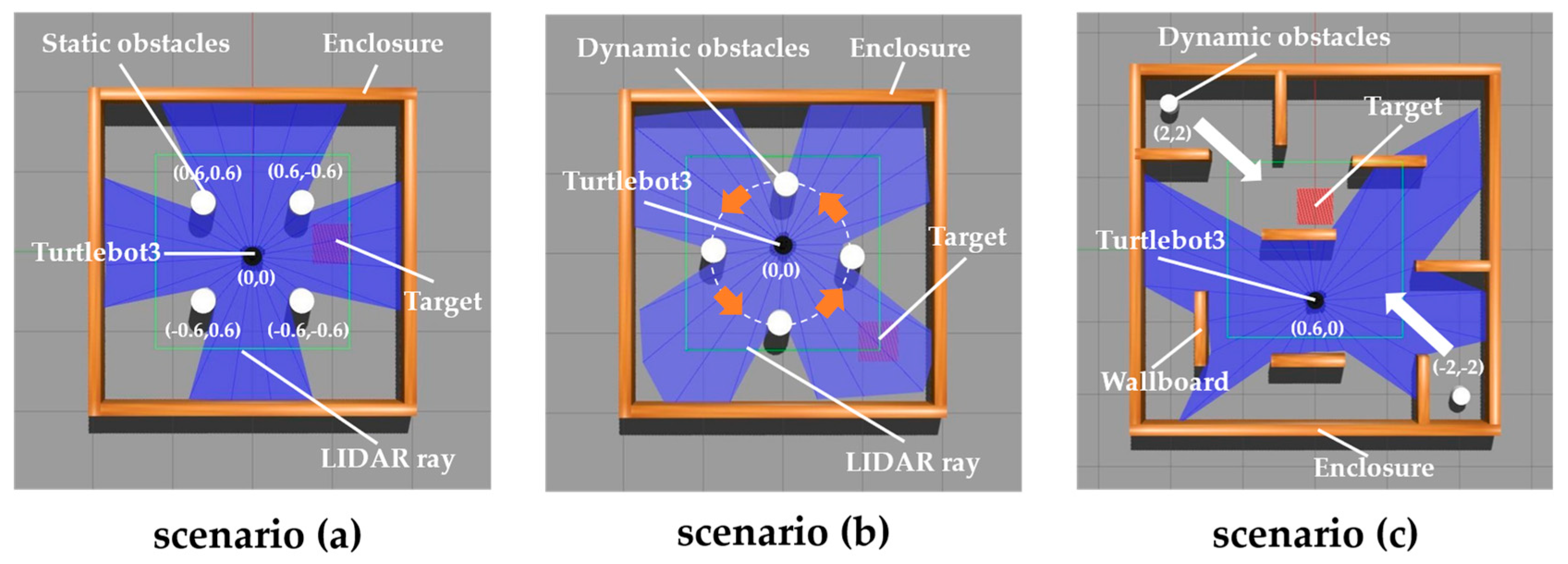
5.2. Experimental Simulation Environment

The experimental environment used in this study is the Gazebo simulation platform, which is known for its highly realistic physical and sensor simulation capabilities. Gazebo can not only accurately simulate physical interactions in the real world, but also allow users to customize complex robot models and environment settings. Its seamless integration with ROS builds a bridge between simulation and real-world applications, and supports parallel interactive and collaborative simulation operations, providing a comprehensive and flexible testing environment for the innovation and verification of robotics technology. Compared with traditional simulation tools, Gazebo has more advanced design and functions, which promotes the rapid development of robotics in research and practical applications. To evaluate the performance of the proposed PER-D2MQN algorithm in local path planning within typical indoor environments, we designed three simulated indoor scenarios. Figure 7 illustrates these scenarios and their layouts, with the starting coordinates of the robot and the coordinates of obstacles indicated in each assumed environment.

1. In scenario (a), the environment is static, with obstacles at fixed positions.

2. In scenario (b), based on the static environment in (a), four white obstacles are set as dynamic obstacles rotating counterclockwise, with an angular velocity of 0.35 rad/s.

3. In scenario (c), two white dynamic obstacles move in random directions.

In each simulation environment, the task for the robot is to start from its initial position, avoid all obstacles, and successfully reach a randomly generated target location.

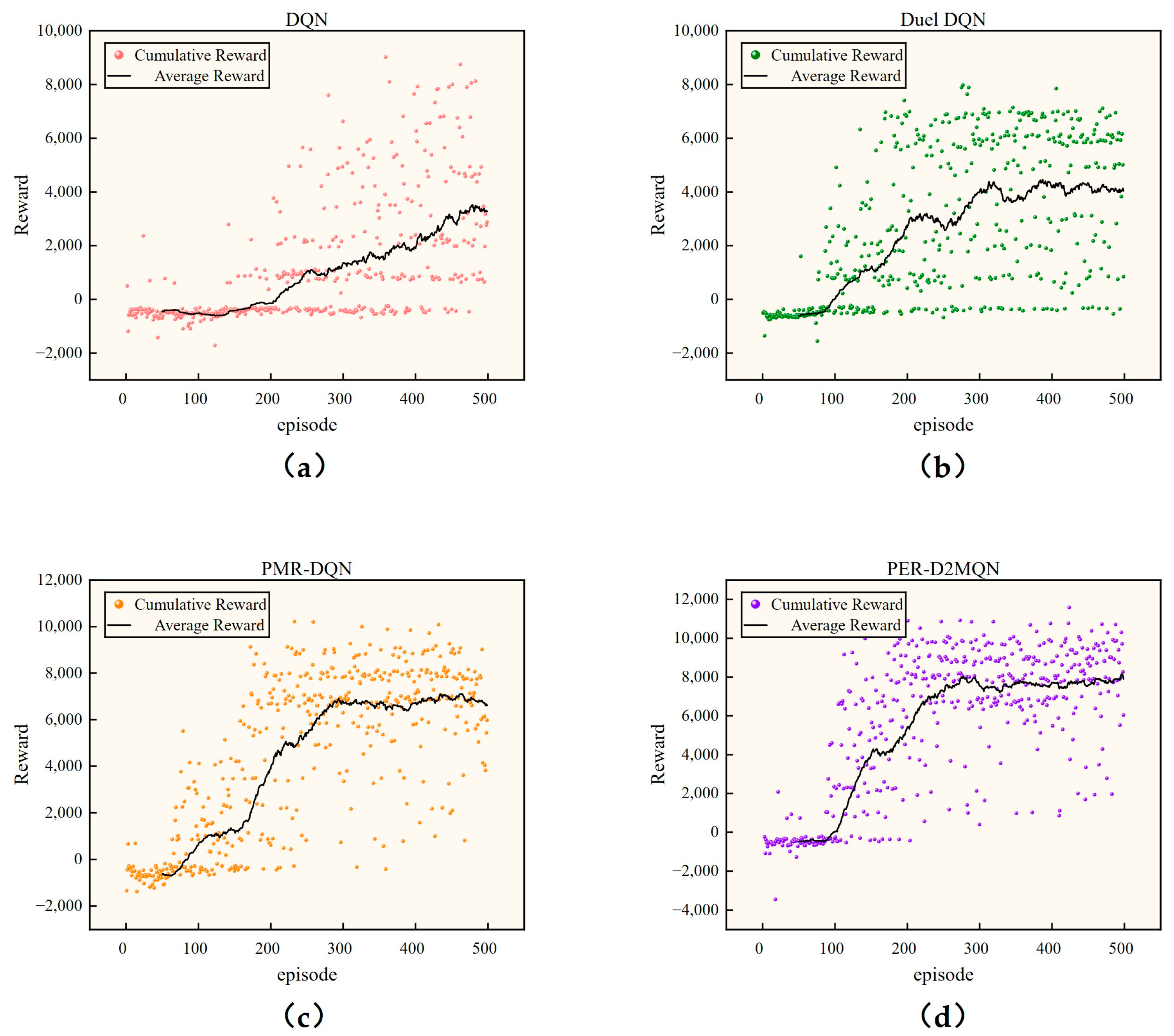
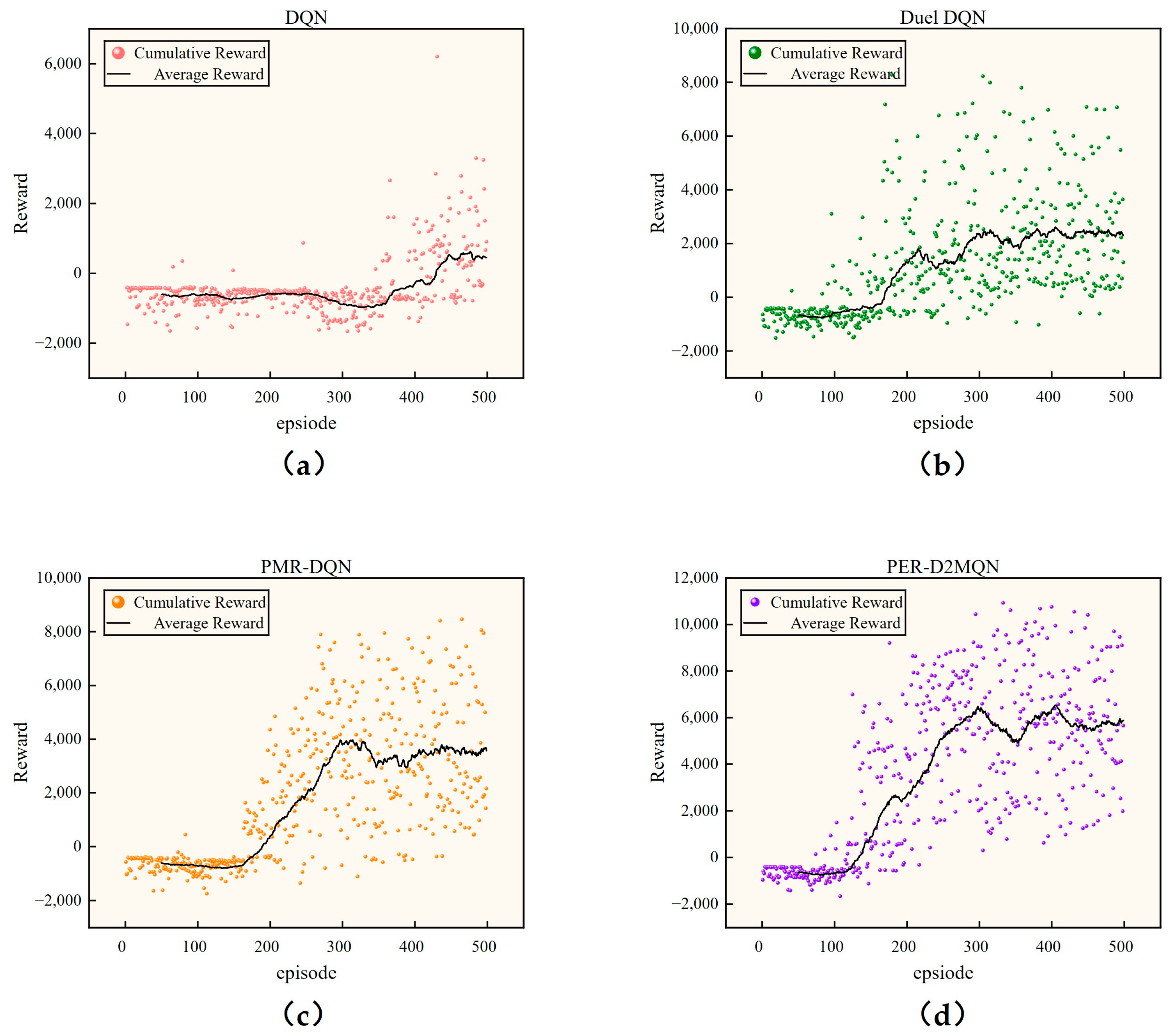
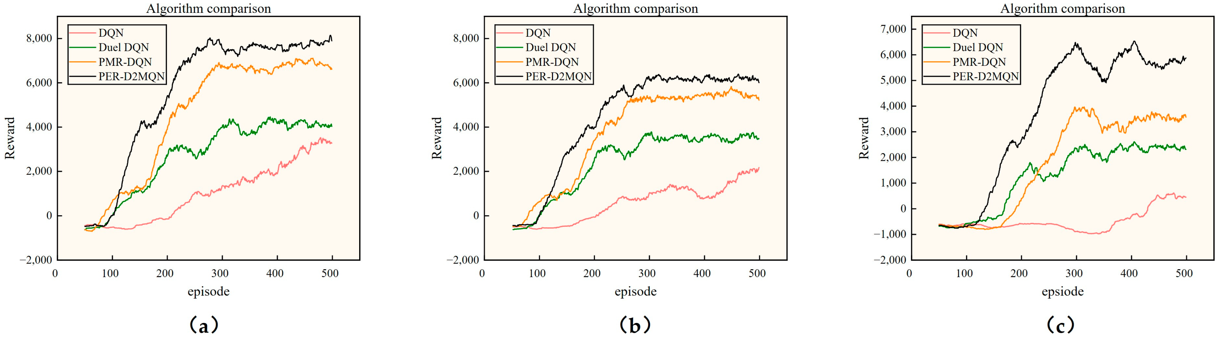
5.3. Simulation Comparison Experiment

We show the cumulative and average rewards obtained by the four algorithms trained based on the model-free approach in the three scenarios (a), (b) and (c) in Figure 8, Figure 9 and Figure 10, respectively, where the cumulative rewards are represented by circular scatters and the average rewards are depicted in a folded line. And the average rewards obtained from the four algorithms trained in the three scenarios are compared in Figure 11. The simulation experiments were all performed within 500 episodes, and an episode was terminated when the robot collided while searching for the target location or when the number of execution steps exceeded 500.

As can be seen in Figure 8, the cumulative reward of the four algorithms in scenarios (a) show some volatility. In terms of average reward, the DQN algorithm has no obvious convergence trend throughout the simulation process; in contrast, the Duel DQN algorithm gradually converges after 300 episodes by changing the network structure, and the average reward tends to be around 4000, but the cumulative reward still fluctuates greatly. The PMR-DQN algorithm, which introduces the PER mechanism, shows better stability, with the average reward gradually converging to around 6700 after 300 episodes, and the fluctuation of the cumulative reward decreases compared with that of Duel DQN. The PER-D2MQN algorithm shows better convergence after 250 episodes, with the average rewards converging to about 7500, and the fluctuation of the cumulative rewards is minimized, which is a significant improvement in the performance. The comparison of the average rewards in Figure 11a further validates these findings.

Figure 9 illustrates the cumulative rewards and average rewards of four algorithms in the scenario (b) with dynamic obstacles. In terms of cumulative rewards, all four algorithms exhibit a certain degree of fluctuation. However, the PMR-DQN and PER-D2MQN algorithms demonstrate significantly better performance, with cumulative rewards appearing more frequently within the range of (4000, 12,000) after 200 episodes. In contrast, the DQN algorithm shows larger fluctuations in cumulative rewards, while Duel DQN exhibits comparatively reduced volatility. Regarding average rewards, the differences between the algorithms are more pronounced. The DQN algorithm does not exhibit a clear trend of convergence throughout the simulation. In contrast, the Duel DQN algorithm begins to converge after 200 episodes, stabilizing around 3700 after 300 episodes. The PMR-DQN algorithm demonstrates better stability, with its average reward gradually converging to approximately 5200 after 260 episodes, while its cumulative reward fluctuations are smaller compared to Duel DQN. Notably, the PER-D2MQN algorithm achieves the best convergence performance, with its average reward stabilizing at around 6200 after 300 episodes. Moreover, it has the smallest cumulative reward fluctuations, indicating significantly improved performance over the other algorithms. The comparison of average rewards in Figure 11b further highlights the superiority of the PER-D2MQN algorithm, as its average reward is consistently higher than those of the other algorithms.

As shown in Figure 10, in the more challenging scenario (c), the DQN algorithm struggles to efficiently locate the target point. Throughout the entire training process, it successfully avoids all obstacles and completes the task in only one episode. In contrast, the other three algorithms demonstrate the ability to complete the task multiple times in this complex environment, with the PER-D2MQN algorithm exhibiting the most remarkable performance. In terms of average rewards, the Duel DQN algorithm begins to converge after 218 episodes, with its average reward stabilizing at approximately 2300. This indicates that the robot performs many inefficient actions while searching for the target point, leading to the identification of only a few target points within a single episode. In comparison, the PMR-DQN and PER-D2MQN algorithms significantly reduce inefficient actions, enabling the robot to locate more target points. Specifically, the PMR-DQN algorithm achieves an average reward of around 4000 after 300 episodes, while the PER-D2MQN algorithm stabilizes its average reward within the range of 4800 to 6000.

Furthermore, Figure 11c provides a more intuitive comparison, clearly showing that the average reward of the PER-D2MQN algorithm is significantly higher than that of the other three algorithms. This demonstrates that, after 500 training episodes in scenario (c), the PER-D2MQN algorithm is not only more efficient at locating target points but also achieves higher rewards per episode, highlighting its distinct advantages.

To further demonstrate the superiority of the PER−D2MQN algorithms, we evaluated the performance of the four algorithms in three scenarios trained with 500 episodes in detail. The evaluation metrics include success rate (the percentage of episodes in which the robot avoids collisions), average steps (the mean number of steps required for the robot to reach the target point in all successful episodes), and average time (the mean time required for the robot to locate the target point in all successful episodes). These metrics comprehensively demonstrate the performance advantages of the PER-D2MQN algorithm from multiple perspectives.

Table 3. Performance comparison of four algorithms in the scenario (a).

Algorithm	Success Rate	Convergence Average Steps	Convergence Average Time/s
DQN	13.6%	161	78
Duel DQN	36.2%	94	45
PMR-DQN	57.6%	74	38
PER-D2MQN	65.8%	64	31

,

Table 4. Performance comparison of four algorithms in the scenario (b).

Algorithm	Success Rate	Convergence Average Steps	Convergence Average Time/s
DQN	9.5%	357	174
Duel DQN	27.7%	144	70
PMR-DQN	46.3%	88	43
PER-D2MQN	52.7%	77	38

and

Table 5. Performance comparison of four algorithms in the scenario (c).

Algorithm	Success Rate	Convergence Average Steps	Convergence Average Time/s
DQN	0.2%	—	—
Duel DQN	12.2%	238	116
PMR-DQN	23.8%	167	81
PER-D2MQN	44.6%	91	44

show the performance parameters of the four algorithms in three scenarios, respectively. It can be clearly seen that the PER-D2MQN algorithm outperforms the other algorithms in all the scenarios. In scenario (a), its success rate reached 65.8%, which was the highest among all algorithms; the average number of steps was 64 and the average time consumed was about 31 s, which were both the lowest. In contrast, the DQN algorithm and the Duel DQN algorithm had success rates of 13.6% and 36.2%, respectively, neither of which exceeded 50% and required significantly more steps and time to complete the task. The PMR-DQN algorithm, with a success rate of 57.6%, had a relatively small number of steps and time consumed, and performed second to the PER-D2MQN algorithm.

In scenario (b), the PER-D2MQN algorithm maintains the best performance with a success rate of 52.7%, an average number of steps of 77, and an average time consumed of 38 s, despite the influence of dynamic obstacles. Facing a more complex and variable scenario (c), the PER-D2MQN algorithm has a 44.6% success rate, which is decreased but significantly better than the other algorithms, especially close to twice the success rate of the PMR-DQN algorithm. In contrast, the remaining three algorithms perform significantly worse in scenario (c).

Notably, the PER-D2MQN algorithm shows relatively small variations in performance parameters across the three scenarios, demonstrating its greater adaptability in complex environments. In addition, for the DQN algorithm in scenario (c), the results are still counted in the calculation of the average number of steps and the average time due to the fact that only one episode succeeded in finding the target point, which is subject to a certain degree of chance. These data further demonstrate the robustness and superiority of the PER-D2MQN algorithm in multi-scene tasks.

Through knowledge transfer learning, previously trained neural network weights are migrated to new training scenarios, thereby accelerating the convergence process and reducing resource consumption. Using a priori knowledge to initialize the network parameters instead of random initialization can significantly improve the performance of reinforcement learning methods in obstacle avoidance tasks and help generate better paths [26,37,38]. Figure 12 illustrates the cumulative reward performance of the PER-D2MQN algorithm with or without applying knowledge transfer learning conditions, where (a) represents the cumulative reward when the robot is directly trained for 500 episodes in scenario (b), and (b) represents the cumulative reward performance when the robot is trained for 500 episodes in scenario (a), then migrates the learned knowledge to scenario (b), and is further trained for 500 episodes.

From Figure 12, it can be seen that after applying knowledge transfer learning, the cumulative reward quickly converges to 8000 after 130 episodes, showing high convergence efficiency. In contrast, without using knowledge transfer learning, the cumulative reward fluctuates between 4000 and 8000 after 200 episodes, with a slower and unstable convergence trend. This suggests that the robot, with prior knowledge of scenario (a), can significantly improve its performance in the training of scenario (b), accelerating the learning process and obtaining better results.

6. Conclusions

This study optimizes and analyzes the application of the DQN algorithm with respect to local path planning for indoor mobile robots. Three key improvements are proposed to address the limitations of the traditional DQN algorithm in path planning: first, the robot’s learning process in complex environments is accelerated by the introduction of the Duel DQN structure; second, the stability and efficiency of the planning process is improved by the use of PER, which increases the efficiency of utilizing key experiences; and third, the robot’s ability to learn the maximum entropy strategy by integrating the maximum entropy strategy from M-DQN into the optimal strategy is significantly improved. Five steering modes are designed to improve the agility of the robot, while a well-designed reward function solves the sparse reward problem. Three scenarios are simulated in the Gazebo simulation environment, and the simulation results show that the proposed PER-D2MQN algorithm significantly outperforms the DQN, Duel DQN, and PMR-DQN in both environments, demonstrating superior performance and potential for practical applications.

Although the PER-D2MQN algorithm shows significant improvements in simulation, there remain issues related to sensor precision and the challenges DRL algorithms face in achieving convergence in high-dimensional spaces, and the success rate of the robot in complex scenarios (c) is only less than 50%, which results in collision risks during local path planning. Therefore, future research will focus on further optimizing the algorithm to enhance its robustness and adaptability in diverse environments. Specific improvements include combining DRL with traditional path planning methods to improve real-time obstacle avoidance capabilities. Additionally, the next steps will involve applying the algorithm to real robots and conducting rigorous testing in both indoor and outdoor environments to validate its generalization ability and optimize performance, thus advancing its practical application.

References

1. Panigrahi, P.K.; Bisoy, S.K. Localization strategies for autonomous mobile robots: A review. J. King Saud Univ.-Comput. Inf. Sci. 2022, 34, 6019–6039. [Google Scholar] [CrossRef]
2. Sánchez-Ibáñez, J.R.; Pérez-del-Pulgar, C.J.; García-Cerezo, A. Path Planning for Autonomous Mobile Robots: A Review. Sensors 2021, 21, 7898. [Google Scholar] [CrossRef] [PubMed]
3. Liu, L.; Wang, X.; Yang, X.; Liu, H.; Li, J.; Wang, P. Path planning techniques for mobile robots: Review and prospect. Expert Syst. Appl. 2023, 227, 120254. [Google Scholar] [CrossRef]
4. Gök, M. Dynamic path planning via Dueling Double Deep Q-Network (D3QN) with prioritized experience replay. Appl. Soft Comput. 2024, 158, 111503. [Google Scholar] [CrossRef]
5. Qin, H.; Shao, S.; Wang, T.; Yu, X.; Jiang, Y.; Cao, Z. Review of Autonomous Path Planning Algorithms for Mobile Robots. Drones 2023, 7, 211. [Google Scholar] [CrossRef]
6. Song, J.; Zhao, M.; Liu, Y.; Liu, H.; Guo, X. Multi-Rotor UAVs Path Planning Method based on Improved Artificial Potential Field Method. In Proceedings of the 2019 Chinese Control Conference (CCC), Guangzhou, China, 27–30 July 2019; pp. 8242–8247. [Google Scholar]
7. Lee, M.-F.R.; Yusuf, S.H. Mobile Robot Navigation Using Deep Reinforcement Learning. Processes 2022, 10, 2748. [Google Scholar] [CrossRef]
8. Mnih, V.; Kavukcuoglu, K.; Silver, D.; Rusu, A.A.; Veness, J.; Bellemare, M.G.; Graves, A.; Riedmiller, M.; Fidjeland, A.K.; Ostrovski, G.; et al. Human-level control through deep reinforcement learning. Nature 2015, 518, 529–533. [Google Scholar] [CrossRef]
9. Wei, Y.; Zheng, R. A Reinforcement Learning Framework for Efficient Informative Sensing. IEEE Trans. Mob. Comput. 2020, 27, 2306–2317. [Google Scholar] [CrossRef]
10. Van Hasselt, H.; Guez, A.; Silver, D. Deep Reinforcement Learning with Double Q-Learning. In Proceedings of the AAAI Conference on Artificial Intelligence, Phoenix, AZ, USA, 12–17 February 2016; Volume 30. [Google Scholar] [CrossRef]
11. Wang, Z.; Schaul, T.; Hessel, M.; van Hasselt, H.; Lanctot, M.; de Freitas, N. Dueling Network Architectures for Deep Reinforcement Learning. arXiv 2016, arXiv:1511.06581. Available online: https://arxiv.org/abs/1511.06581 (accessed on 14 July 2024).
12. Kim, H.; Lee, W. Dynamic Obstacle Avoidance of Mobile Robots Using Real-Time Q Learning. In Proceedings of the 2022 International Conference on Electronics, Information, and Communication (ICEIC), Jeju, Republic of Korea, 6–9 February 2022; IEEE: New York, NY, USA, 2022; pp. 1–2. [Google Scholar]
13. Wang, C.; Yang, X.; Li, H. Improved Q Learning Applied to Dynamic Obstacle Avoidance and Path Planning. IEEE Access 2022, 10, 92879–92888. [Google Scholar] [CrossRef]
14. Zhou, Q.; Lian, Y.; Wu, J.; Zhu, M.; Wang, H.; Cao, J. An optimized Q Learning algorithm for mobile robot local path planning. Knowl.-Based Syst. 2024, 286, 111400. [Google Scholar] [CrossRef]
15. Orozco-Rosas, U.; Picos, K.; Pantrigo, J.J.; Montemayor, A.S.; Cuesta-Infante, A. Mobile Robot Path Planning Using a QAPF Learning Algorithm for Known and Unknown Environments. IEEE Access 2022, 10, 84648–84663. [Google Scholar] [CrossRef]
16. Schaul, T.; Quan, J.; Antonoglou, I.; Silver, D. Prioritized Experience Replay. arXiv 2016, arXiv:1511.05952. Available online: https://arxiv.org/abs/1511.05952 (accessed on 15 July 2024).
17. Haarnoja, T.; Zhou, A.; Abbeel, P.; Levine, S. Soft Actor-Critic: Off-Policy Maximum Entropy Deep Reinforcement Learning with a Stochastic Actor. In International Conference on Machine Learning, Proceedings of the 35th International Conference on Machine Learning (ICML), Stockholm, Sweden, 10–15 June 2018; Dy, J., Krause, A., Eds.; JMLR-Journal Machine Learning Research: San Diego, CA, USA, 2018; Volume 80, Available online: https://webofscience.clarivate.cn/wos/alldb/full-record/WOS:000683379201099 (accessed on 15 July 2024).
18. Vieillard, N.; Pietquin, O.; Geist, M. Munchausen Reinforcement Learning. Adv. Neural Inf. Process. Syst. 2020, 33, 4235–4246. [Google Scholar]
19. Liu, S.; Zheng, C.; Huang, Y.; Quek, T.Q. Distributed Reinforcement Learning for Privacy-Preserving Dynamic Edge Caching. IEEE J. Sel. Areas Commun. 2022, 40, 749–760. [Google Scholar] [CrossRef]
20. Han, H.; Wang, J.; Kuang, L.; Han, X.; Xue, H. Improved Robot Path Planning Method Based on Deep Reinforcement Learning. Sensors 2023, 23, 5622. [Google Scholar] [CrossRef]
21. Zhang, F.; Gu, C.; Yang, F. An Improved Algorithm of Robot Path Planning in Complex Environment Based on Double DQN. arXiv 2021, arXiv:2107.11245. [Google Scholar]
22. Yang, Y.; Wang, J.; Zhang, H.; Dai, S. Path planning of mobile robot based on improved DDQN. J. Phys. Conf. Ser. 2024, 2021, 012029. [Google Scholar] [CrossRef]
23. Gu, Y.; Zhu, Z.; Lv, J.; Shi, L.; Hou, Z.; Xu, S. DM-DQN: Dueling Munchausen deep Q network for robot path planning. Complex Intell. Syst. 2023, 9, 4287–4300. [Google Scholar] [CrossRef]
24. Kong, F.; Wang, Q.; Gao, S.; Yu, H. B-APFDQN: A UAV Path Planning Algorithm Based on Deep Q-Network and Artificial Potential Field. IEEE Access 2023, 11, 44051–44064. [Google Scholar] [CrossRef]
25. Li, J.; Shen, D.; Yu, F.; Zhang, R. Air Channel Planning Based on Improved Deep Q Learning and Artificial Potential Fields. Aerospace 2023, 10, 758. [Google Scholar] [CrossRef]
26. Li, W.; Yue, M.; Shangguan, J.; Jin, Y. Navigation of Mobile Robots Based on Deep Reinforcement Learning: Reward Function Optimization and Knowledge Transfer. Int. J. Control. Autom. Syst. 2023, 21, 563–574. [Google Scholar] [CrossRef]
27. Sivaranjani, A.; Vinod, B. Artificial Potential Field Incorporated Deep-Q-Network Algorithm for Mobile Robot Path Prediction. Intell. Autom. Soft Comput. 2023, 35, 1135–1150. [Google Scholar] [CrossRef]
28. Han, Q.; Feng, S.; Wu, X.; Qi, J.; Yu, S. Retrospective-Based Deep Q Learning Method for Autonomous Pathfinding in Three-Dimensional Curved Surface Terrain. Appl. Sci. 2023, 13, 6030. [Google Scholar] [CrossRef]
29. Tu, G.-T.; Juang, J.-G. UAV Path Planning and Obstacle Avoidance Based on Reinforcement Learning in 3D Environments. Actuators 2023, 12, 57. [Google Scholar] [CrossRef]
30. Xie, R.; Meng, Z.; Zhou, Y.; Ma, Y.; Wu, Z. Heuristic Q Learning based on experience replay for three-dimensional path planning of the unmanned aerial vehicle. Sci. Prog. 2020, 103, 003685041987902. [Google Scholar] [CrossRef]
31. Yao, J.; Li, X.; Zhang, Y.; Ji, J.; Wang, Y.; Zhang, D.; Liu, Y. Three-Dimensional Path Planning for Unmanned Helicopter Using Memory-Enhanced Dueling Deep Q Network. Aerospace 2022, 9, 417. [Google Scholar] [CrossRef]
32. Lin, C.-J.; Jhang, J.-Y.; Lin, H.-Y.; Lee, C.-L.; Young, K.-Y. Using a Reinforcement Q Learning-Based Deep Neural Network for Playing Video Games. Electronics 2019, 8, 1128. [Google Scholar] [CrossRef]
33. Zhou, Z.; Zhu, P.; Zeng, Z.; Xiao, J.; Lu, H.; Zhou, Z. Robot navigation in a crowd by integrating deep reinforcement learning and online planning. Appl. Intell. 2022, 52, 15600–15616. [Google Scholar] [CrossRef]
34. Almazrouei, K.; Kamel, I.; Rabie, T. Dynamic Obstacle Avoidance and Path Planning through Reinforcement Learning. Appl. Sci. 2023, 13, 8174. [Google Scholar] [CrossRef]
35. Kamalova, A.; Lee, S.G.; Kwon, S.H. Occupancy Reward-Driven Exploration with Deep Reinforcement Learning for Mobile Robot System. Appl. Sci. 2022, 12, 9249. [Google Scholar] [CrossRef]
36. Gu, S.; Holly, E.; Lillicrap, T.; Levine, S. Deep reinforcement learning for robotic manipulation with asynchronous off-policy updates. In Proceedings of the 2017 IEEE International Conference on Robotics and Automation (ICRA), Singapore, 29 May–3 June 2017; IEEE: Singapore, 2017; pp. 3389–3396. [Google Scholar]
37. Gao, J.; Ye, W.; Guo, J.; Li, Z. Deep reinforcement learning for indoor mobile robot path planning. Sensors 2020, 20, 5493. [Google Scholar] [CrossRef] [PubMed]
38. Matej, D.; Skocaj, D. Deep reinforcement learning for map-less goal-driven robot navigation. Int. J. Adv. Robot. Syst. 2021, 18, 1–13. [Google Scholar] [CrossRef]
Figure 1. Overall flow chart of local path planning based on PER-D2MQN algorithm.
Applsci 14 11195 g001
Figure 2. Markov-based RL process.
Applsci 14 11195 g002
Figure 3. The network structure of the adopted Duel DQN.
Applsci 14 11195 g003
Figure 4. The updating process of the experience vector at moment t.
Applsci 14 11195 g004
Figure 5. Turtlebot3 robot turning direction.
Applsci 14 11195 g005
Figure 6. Turtlebot3 robot state space in the Gazebo environment.
Applsci 14 11195 g006
Figure 7. Gazebo experiment environment. (a) is the experimental static environment (4–4 m); (b) is the experimental dynamic environment (4–4 m); (c) is the experimental complex environment (5–5 m).
Applsci 14 11195 g007
Figure 8. Total and cumulative rewards generated by the four algorithms for each episode in Env1. (a) represents the cumulative reward and average reward plots of the DQN; (b) represents the cumulative reward and average reward plots of the Duel DQN; (c) represents the cumulative reward and average reward plots of the PMR−DQN; (d) represents the cumulative reward and average reward plots of the PER−D2MQN.
Applsci 14 11195 g008
Figure 9. Total and cumulative rewards generated by the four algorithms for each episode in Env2. (a) represents the cumulative reward and average reward plots of the DQN; (b) represents the cumulative reward and average reward plots of the Duel DQN; (c) represents the cumulative reward and average reward plots of the PMR−DQN; (d) represents the cumulative reward and average reward plots of the PER−D2MQN.
Applsci 14 11195 g009
Figure 10. Total and cumulative rewards generated by the four algorithms for each episode in Env3. (a) represents the cumulative reward and average reward plots of the DQN; (b) represents the cumulative reward and average reward plots of the Duel DQN; (c) represents the cumulative reward and average reward plots of the PMR−DQN; (d) represents the cumulative reward and average reward plots of the PER−D2MQN.
Applsci 14 11195 g010
Figure 11. Comparison of average rewards of four algorithms. (a) is the average reward comparison in scenario (a); (b) is the average reward comparison in scenario (b); (c) is the average reward comparison in scenario (c).
Applsci 14 11195 g011
Figure 12. Cumulative rewards of the PER-D2MQN algorithm in scenario (b). (a) Cumulative rewards without the use of transfer learning; (b) cumulative rewards using transfer learning.
Applsci 14 11195 g012