Article

Walking Back the Data Quantity Assumption to Improve Time Series Prediction in Deep Learning

Faculty of Law, Business and Government, Universidad Francisco de Vitoria, 28223 Madrid, Spain
*
Author to whom correspondence should be addressed.
Appl. Sci. 2024, 14(23), 11081; https://doi.org/10.3390/app142311081
Submission received: 28 October 2024 / Revised: 21 November 2024 / Accepted: 26 November 2024 / Published: 28 November 2024

Abstract

:
Deep learning techniques have significantly advanced time series prediction by effectively modeling temporal dependencies, particularly for datasets with numerous observations. Although larger datasets are generally associated with improved accuracy, the results of this study demonstrate that this assumption does not always hold. By progressively increasing the amount of training data in a controlled experimental setup, the best predictive metrics were achieved in intermediate iterations, with variations of up to 66% in RMSE and 44% in MAPE across different models and datasets. The findings challenge the notion that more data necessarily leads to better generalization, showing that additional observations can sometimes result in diminishing returns or even degradation of predictive metrics. These results emphasize the importance of strategically balancing dataset size and model optimization to achieve robust and efficient performance. Such insights offer valuable guidance for time series forecasting, especially in contexts where computational efficiency and predictive accuracy must be optimized.

1. Introduction

Deep learning has made remarkable strides in time series prediction, largely due to its ability to model complex temporal dependencies that traditional methods often struggle with. The evolution of deep learning architectures for time series forecasting began with multilayer perceptrons (MLPs), which laid the groundwork for later developments in the field. MLPs [1,2,3,4] enabled the modeling of static relationships in data, but as the need for capturing sequential information arose, more sophisticated techniques were developed. This led to the advent of recurrent neural networks (RNNs) [5,6] which incorporate feedback loops to retain information from past states, significantly enhancing predictive capabilities. The field continues to progress with the introduction of transformer networks [7,8] which have shown exceptional performance in a variety of tasks, including time series forecasting, by allowing for long-range dependencies without the limitations of sequential processing inherent in RNNs.
Modern deep learning models, particularly large language models (LLMs) [9], have architectures that can include billions of parameters, reinforcing the principle of “more data, better model performance”. This principle posits that increasing the amount of training data generally leads to improvements in model accuracy, yet this can be challenging in practice.
Despite these advancements in architecture, a significant research gap remains regarding the optimal use of data volume in training deep learning models for time series forecasting. Although the prevailing assumption in the field is that increasing the amount of training data improves model accuracy, this approach has limitations. Large datasets introduce challenges such as noise, missing values, and computational complexity, which may hinder performance and create inefficiencies. Furthermore, traditional learning frameworks like the probably approximately correct (PAC) learning theory [10] suggest that while large sample sizes improve the likelihood of accurate learning, unique challenges arise in time series data, including autocorrelation, non-stationarity, and seasonality [11]. Time series data often exhibit behavioral shifts, where only specific subsets of data may be relevant for making accurate forecasts.
Innovative strategies have emerged to mitigate the limitations associated with small datasets while leveraging the potential of large models. For example, recent findings indicate that thoughtful optimization of model architecture and training processes can yield high accuracy, even with limited data availability [12]. These insights suggest that while the volume of data typically enhances model performance, effective model tuning and the utilization of pre-existing knowledge can reduce the dependence on extensive datasets, making deep learning techniques more applicable across domains where data may be scarce.
The existing literature largely overlooks the possibility that effective training could be achieved with subsets of data, especially when historical data from previous horizons is strategically incorporated. This study addresses this gap by questioning whether the principle of “the more data, the better model performance” holds in the context of time series forecasting. Specifically, it explores whether training deep learning models on selectively chosen subsets provides improved performance metrics compared to training on complete datasets.
Although models are studied in which research focuses on estimating model parameters by using a partial window of available observations [13], if the first available data follow a process unrelated to the current reality, then the use of such data in the estimation can lead to biased predictions and report higher mean square errors. Excessive reduction, however, can negatively impact the variance, reflecting higher errors. For these reasons, it is essential to study methodologies that allow starting from the most recent data and studying the impact of adding mobile windows with historical data to build forecasts, allowing the generalization capacity of the model to be observed [14].
This research, therefore, aims to challenge the traditional view of data quantity and emphasize the potential of optimized training and strategic data usage. By doing so, this study contributes a novel methodology for data selection in deep learning for time series forecasting, demonstrating that, in some cases, intermediate dataset sizes yield optimal predictive accuracy. The key contributions of this study are as follows:
This work critically examines the impact of dataset size on time series forecasting using deep learning techniques. Through an experimental approach, it is demonstrated that optimal predictive performance is not always achieved with the complete dataset, but rather in intermediate iterations, challenging the assumption that larger datasets always yield better metrics. The key contributions of this study are as follows:
-
Identification of a nonlinear relationship between dataset size and predictive performance, with significant variations in metrics such as RMSE (up to 66%) and MAPE (up to 44%) across different models and time series.
-
Proposal of a methodology that optimizes data usage, illustrating how strategic selection of observations can enhance computational efficiency without compromising model accuracy.
-
Demonstration that, in certain cases, smaller datasets can outperform larger ones in terms of overall model performance, depending on the time series structure and the model employed.
This article is organized as follows: Section 2 provides a detailed description of the methodology. Section 3 gives information on the databases used and details of the parameters of the models employed. Section 4 focuses on the main results. Section 5 presents a discussion based on the obtained evidence. Finally, Section 6 describes the conclusions and future lines of work.

2. Related Works

In recent years, machine learning (ML) models have increasingly leveraged metaheuristic algorithms for fine-tuning, enhancing their predictive accuracy and efficiency, particularly in time series forecasting. Metaheuristic approaches, including genetic algorithms, particle swarm optimization, and simulated annealing, offer robust solutions for optimizing the hyperparameters of complex models [15]. This is especially beneficial in fields where data characteristics are highly dynamic, such as financial forecasting and hydrological predictions [16]. For instance, in forecasting cryptocurrency prices, decomposition-aided long short-term memory (LSTM) models, tuned with metaheuristic algorithms, have shown promise in capturing volatile patterns in bitcoin pricing [17]. This approach not only enhances model performance, but also facilitates interpretability through techniques such as Shapley values, which provide insights into feature contributions to model predictions.
The combination of deep learning architectures with metaheuristic optimization has also seen success in environmental sciences, particularly for streamflow and hydroclimatic data analysis. Recent studies demonstrate that by incorporating metaheuristic-enhanced ML models, such as those using gradient-boosted trees and deep neural networks, researchers can significantly improve monthly streamflow prediction [18]. These models, tuned to capture intricate hydroclimatic dependencies, underscore the potential of metaheuristics in adapting ML models to unique domain challenges. As a result, the use of metaheuristics for model optimization has emerged as a state-of-the-art approach in time series forecasting, offering a more adaptable and fine-grained methodology that enhances both accuracy and applicability across diverse domains.

2.1. Neural Networks for Time Series Forecasting

The large amount of available data makes ANNs increasingly a dominant technique in time series predictions. There is a wide literature on the use of neural networks, Zhang [19] makes an extensive summary of works in which different models are applied to these tasks, obtaining results with lower errors than traditional techniques.
In the model studied by Hochreiter and Schmidhuber [20], a long-term memory network (LSTM) has the capacity to store information from iterations in the network, behaving as a memory of the previous states to calculate the following states.
Several researchers have described the performance of LSTM networks for the prediction of time series, such as those observed in [21,22,23], discovering a higher performance than traditional techniques, especially in cases of large numbers of observations. The use of BiLSTM networks, although also widely extended and with good results, is not contemplated since it would increase the processing time and the computational cost [24], without a significant improvement in the results.
A simpler architecture is the MLP, one of the most studied networks in the literature due to its simplicity in time series prediction tasks [25,26,27], in addition to the great ability to establish relationships despite being the simplest model, it is currently still the subject of extensive research. This widespread use is due to the fact that it is a simple, but highly effective model [28], especially in the approximation of functions even in non-linear time series or with missing data.

2.2. Impact of Data Quantity in Time Series Forecasting

In time series forecasting, the correlation between the quantity of data and model accuracy is particularly pronounced. Larger datasets are often essential for accurately modeling complex multivariate time series, as they capture a wider array of seasonal and cyclical patterns. For instance, models such as DeepAR [29] demonstrate enhanced performance when trained on extensive historical datasets, allowing them to identify intricate temporal dependencies. In financial forecasting, longer and richer multivariate time series provide the necessary context for models like long short-term memory (LSTM) networks, thereby improving predictive accuracy [30].
However, the utilization of larger datasets is not without its challenges. Issues such as noise, missing data, and the computational complexity of handling vast datasets can hinder model performance. To address these concerns, techniques such as data imputation and noise filtering have been explored to enhance the quality of the data used for training.
There is some concern in the literature about the number of observations needed to obtain good predictions, with some experimentation in this regard through performance measurement and variation of error metrics [31,32], finding significant differences between the observations considered necessary.

2.3. Transfer Learning and Multi-Task Learning

Some authors propose methodologies that try to address the handling of large amounts of data, such as transfer learning [33] which represents a pivotal advancement in model training, allowing practitioners to leverage knowledge from large, pre-existing datasets to improve performance on smaller, domain-specific tasks. Recent studies have demonstrated that pre-training models on external datasets followed by fine-tuning on target datasets can yield significant performance enhancements, particularly when the target data are limited [34]. An example of this is the N-BEATS architecture [35], which has shown improved forecasting accuracy across various domains when pre-trained on general datasets.
In addition, multi-task learning frameworks [36] have emerged as a promising avenue for enhancing predictive performance. By training models on multiple related tasks simultaneously, these frameworks enable the capture of shared patterns across diverse time series datasets, leading to improved outcomes on individual forecasting tasks [37].

2.4. Rolling Window Validation

Other techniques focus on an iterative approach to training to improve predictions. Rolling window validation has emerged as a fundamental technique for evaluating the performance of deep learning models in time series forecasting from the challenge of time-dependent data. This approach involves sequentially training models on a fixed-size training set while testing them on subsequent time periods, effectively simulating real-world forecasting scenarios [38]. Employing rolling windows can ensure that model assessments are robust and reflect the dynamic nature of time series data, which may exhibit non-stationarity, seasonality, and trend shifts over time [39].
Recent studies have highlighted the advantages of rolling window validation over traditional fixed-split methods, as it allows for continuous updates to model parameters and hyperparameters, facilitating the capture of evolving patterns within the data [40]. Additionally, this methodology enhances the generalizability of models by providing multiple evaluations across different temporal segments, ultimately leading to more reliable insights into model performance [41]. Notably, advancements in deep learning architectures, such as LSTMs and transformers, have underscored the importance of effective validation strategies, with rolling window validation being integral to optimizing model training and selection processes in various forecasting applications [42].
All these methodologies are based on the principle of the impact of the size of the time series on predictive models, some focusing on iterative training that includes the most recent observations. The proposed model focuses on a methodology that begins by training with the most recent data [43], allowing the model’s behavior to be observed by adding historical data, obtaining on the one hand information on the model’s ability to generalize by incorporating more data, and on the other hand understanding whether the data history generates an impact on the prediction capacity.

3. Methodology

3.1. Multilayer Perceptron (MLP) Networks

Multilayer perceptron (MLP) models can be considered a classic neural network approach for economic time series forecasting, widely used in the literature [28,44,45,46,47,48]. The main reason for their extensive use is that they are considered universal approximators meaning they can approximate any continuous function with a hidden layer, provided it has enough neurons. Despite their simple and easily programmable structure [3,25], they are the subject of numerous research studies [27], showing promising results.
The processing units that constitute the network (neurons) are structured into multiple layers, hence the term “multilayer”. The first layer represents the input data fed into the neural network, while the final layer is responsible for producing an output that corresponds to the network’s response to the processed data. Between these two, there may be one or more intermediate layers. Each neuron in each layer processes the information it receives from all the neurons in the preceding layer:
x j l = f i w j i l x i l 1 + b j .
In this equation, x j l represents the output of neuron j in layer l. This output is derived from the outputs of neurons in the previous layer, x i l 1 , which are multiplied by the weights w j i l , representing the connections between this neuron and those in the preceding layer. For this reason, these layers are often referred to as dense layers [49]. The output x j l is calculated by applying an activation function f () to the weighted sum of the inputs plus a bias term bj. In hidden layers, common activation functions include the hyperbolic tangent or the sigmoid function, while a linear function is generally used in the output layer.
The power of neural models, such as MLPs, lies in their ability to learn from data, enabling them to perform artificial intelligence tasks. Therefore, it is essential to train them before use. In this process, the available data are split into two groups: one for training and another for validation. The validation set is used to assess the performance of the trained network, which is a standard procedure in neural models.
During training, the data are organized into pairs of inputs and desired outputs. These data are fed into the network, which generates an output. This output is then compared to the expected one to compute the error. The error is propagated backward through the layers to adjust the weights of the neurons to minimize it. The algorithm that performs this adjustment is known as “backpropagation” [50].

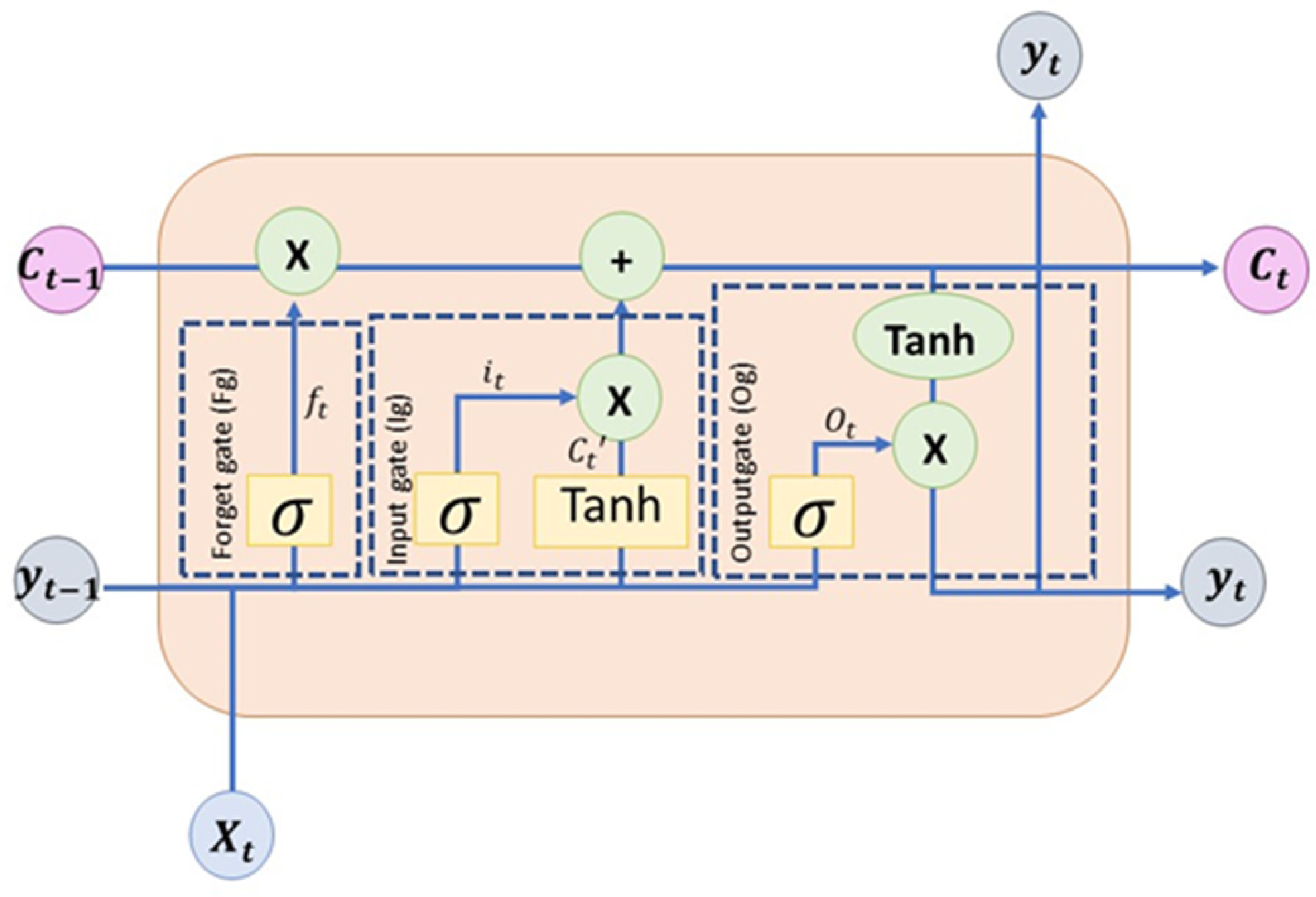
3.2. Long Short-Term Memory (LSTM) Networks

Long short-term memories (LSTMs) are a sophisticated neural network architecture designed to handle time-dependent data such as text, speech, or translations [20]. These networks are equipped with internal memory and feedback loops within neurons in the same layer, allowing them to process sequences effectively. Due to their complexity, the processing units in LSTMs are referred to as “cells” instead of neurons. As depicted in Figure 1, the temporal dynamics of inputs (xt), outputs (yt), feedback (yt−1), and memory states (ct−1 and ct) are clearly illustrated. Each cell contains three gates, the input gate, forget gate, and output gate, which regulate the flow of data within the cell over time. These gates determine how much of the information is used to update the internal state.
The forget gate is responsible for deciding whether to retain or discard the stored information, ct−1. This decision is made by computing the weighted sum of the new inputs, xt, and the outputs from all neurons in the preceding time step, yt−1. This computation is processed through a sigmoid function σ , which produces a response ranging from 0 (indicating complete erasure of the “memory”) to 1 (indicating full retention of the “memory”):
f t = σ ( W f y t 1 , x t + b f ) ,
In this expression, y t 1 , x t represents the input vector (column vector) to the cell, comprising the new inputs at time t, x t , and the outputs of all neurons in the same layer at the previous time step, y t 1 (feedback). The symbol Wf denotes the weight vector associated with the forget gate, which includes weights for both the new inputs and the feedback, while bf signifies the corresponding bias. It is important to note that in neural network literature, weights are typically represented as matrices when referring to an unspecified neuron within a layer, with each row corresponding to a specific neuron. However, since the formula reflects the response of a single neuron, the weight matrix is represented as a row vector, which is then multiplied (through the dot or scalar product) by the column vector comprising the new inputs and feedback.
The input gate determines whether to incorporate new information into the internal state of the cell (its “memory”). Similarly, the weighted sum of new inputs and feedback is processed through a sigmoid function to ascertain the extent to which new information should be integrated into the cell’s “memory”:
i t = σ ( W i y t 1 , x t + b i ) ,
In this context, Wi and bi represent the associated weight matrix and bias. The information intended for inclusion in the cell’s “memory” is calculated using the hyperbolic tangent function, which yields values ranging from −1 to +1. This is applied to the weighted sum (with Wc as the weight matrix) of the new information supplied to the cell, in conjunction with contributions from other neurons within the same layer. A bias term, bc, is also incorporated in this computation:
c t = tanh W c y t 1 , x t + b c .
The updated internal state is derived from the combination of the portion of its prior value preserved by the forget gate and the input of the new information supplied by the input gate. Therefore, it can be expressed in the following manner:
c t = f t c t 1 + i t c t .
The output gate determines the proportion of the new internal state that will be emitted as the cell’s output. This value, which ranges from 0 to 1, is obtained through a sigmoid function that processes the weighted sum of the new input data (Wo is the weight matrix) and the previous outputs of the neurons in the same layer, in addition to a bias term (bo). This approach is consistent with the processing methods used for the other gates (i.e., the forget gate and the input gate, ft and it):
o t = σ W o y t 1 , x t + b o .
The output of the new cell will be the portion of the hyperbolic tangent of the new internal state that the output gate permits to be transmitted.
y t = o t tanh ( c t ) .
LSTM is trained using a variant of the traditional backpropagation algorithm, specifically tailored to accommodate the recurrent architecture of this model. This training process involves two key modifications: the truncated backpropagation through time (BPTT), which is employed to update the weights associated with the output units and output gates, and the real-time recurrent learning (RTRL), which focuses on adjusting the weights of the cell inputs, input gates, and forget gates [21].

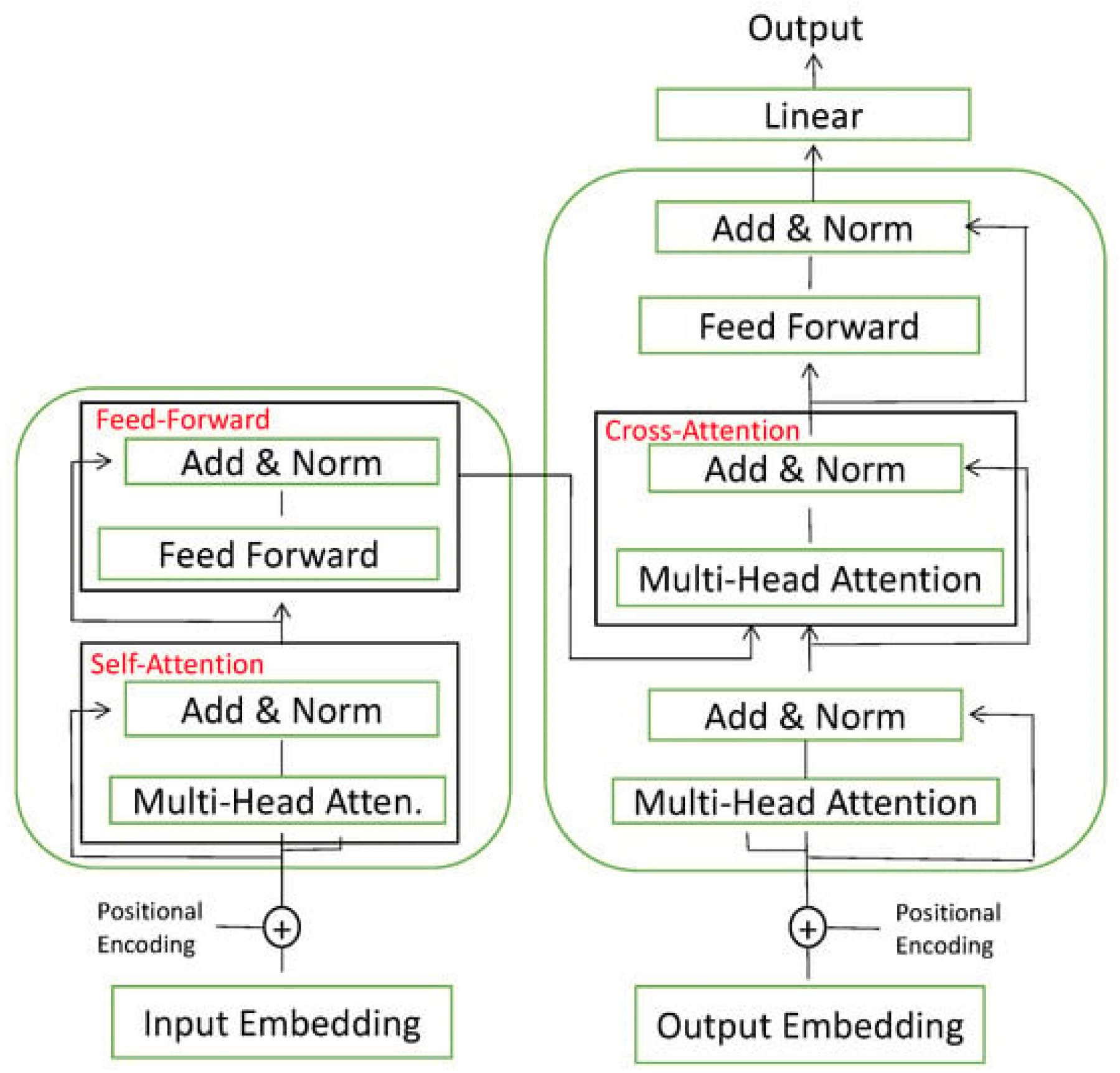
3.3. Transformer Networks
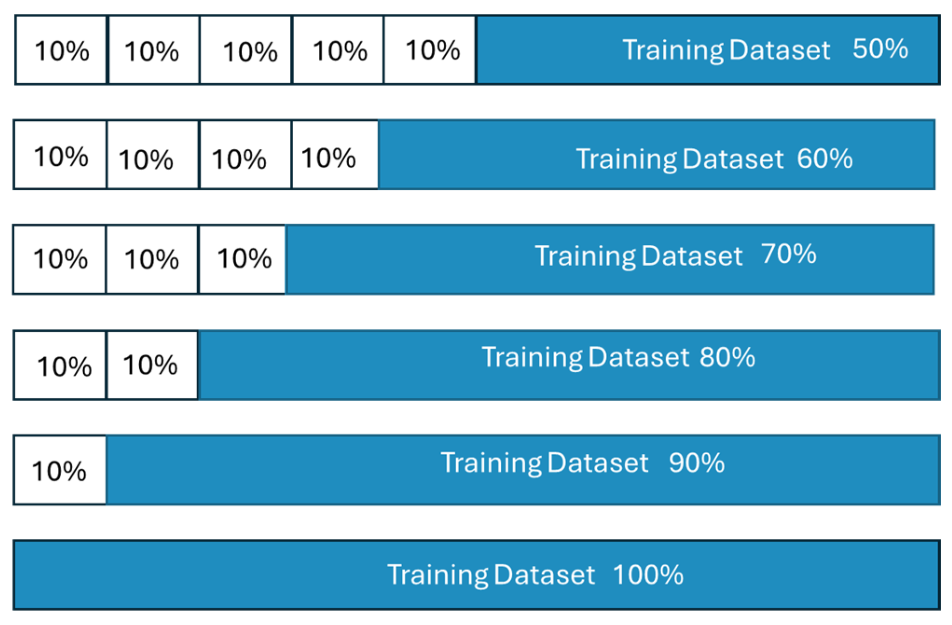
In recent years, the use of transformer-based models for time series forecasting has grown exponentially, as these solutions are particularly effective in extracting correlations within long time series. Previously, these techniques were primarily utilized in the fields of natural language processing (NLP) and computer vision [51,52] which has led to an increasing interest in these networks due to their ability to capture dependencies and interactions for forecasting time series.
Transformer architectures are characterized by their encoder–decoder structure, represented in Figure 2, where each encoder layer generates information regarding the relevance of the inputs among themselves. Conversely, the decoder layer performs the opposite function: based on the encodings, it generates the output sequence using the embedded contexts [53].
The application of transformers for time series prediction is on the rise, as evidenced by the increasing number of publications focused on this area and the promising results obtained [54,55] solidifying this model as an attractive alternative to traditional approaches [56].
These networks possess a deep learning architecture based on attention mechanisms. The introduction of scaled dot-product attention algorithms is grounded in the research conducted by Vaswani [57], whose primary objective was to enable models to focus on the most relevant elements. To achieve this, the weighted sum of the values (V) is calculated, where the weights are obtained through the softmax function applied to the dot products of the queries (Q) and keys (K), scaled by the square root of the dimension of the keys (dk).

3.4. Walking Back

The proposed methodology is based on the hypothesis that a larger number of observations increases both the computational cost and the training time of the models, without necessarily guaranteeing an improvement in predictive performance. This phenomenon is because, although more data can provide more information, they can also increase the complexity of the model, which can lead to overfitting, where the model learns non-generalizable patterns from the training data.
There is a gap in the literature regarding the optimal number of observations needed to efficiently train neural networks. This ideal amount is not universal and depends largely on the characteristics inherent to the time series, such as its seasonality, trends, periodicity, and noise level. Previous studies have shown that the optimal amount of training data is not always linearly proportional to the accuracy of the models, as performance can degrade when irrelevant or excessively noisy historical data are introduced.
The choice to split the time series in half (50%) as a starting point is based on the search for a balance between the amount of data used for training and the amount reserved for subsequent iterations. Fifty percent represents a compromise between a sample large enough to capture general patterns and an appropriate starting point for progressive evaluation, avoiding computational overhead from the start. Various studies in incremental learning suggest that splitting the data into large initial segments can help identify the point at which the model starts to overfit historical data rather than improve performance.
By splitting only half of the observations, the model has enough information to learn general relationships in the time series without being overly dependent on noisy or irrelevant patterns in the early data. In fact, in many cases of time series prediction, more recent data tend to have more relevance in future prediction than distant historical data, making a progressive and selective approach to data input appropriate. This is also aligned with the practice of using moving or dynamic data windows, widely used in time series forecasting, which suggests that using recent data may be more beneficial than including the entire series.
The progressive inclusion of the additional 10% of data in each iteration allows for a flexible and adaptive approach to model evaluation, as one can monitor at each step how the model’s performance changes as more historical data are introduced. This approach is derived from the methodology of cross-validation and learning curve analysis, where the idea is to find the point at which the model reaches its optimal performance without the addition of additional data generating substantial improvements. In some cases, adding more data can even degrade performance due to the phenomenon known as diminishing returns [58], which occurs when additional data brings redundant information or noise that reduces the model’s ability to generalize. The sequence of action of the model is reflected in Figure 3.
Formally, let x = { x 1 , , x N   } R N by the full time series where N is the total number of time steps. Each iteration k { 1 ,   2 ,   3 ,   4 ,   5 ,   6 } defines a subset x ( k ) of the full time series as:
x ( k ) = x N 2 + 1 ( k 1 ) N 10 , , x ( N )

4. Dataset Details and Performance Metrics

4.1. Dataset

This section describes the time series used in the experimentation process to verify the results with the ANNs used: MLP, LSTM, and transformer. These are data with different characteristics, especially the number of observations, to check how the new methodology influences when it comes to obtaining the best results.
The first time series included in the study is the time series with prices from NEMO (nominated electricity market operator) for the management of the daily and intraday market for electricity prices. The large number of observations contained in this dataset allows a contrast with smaller time series. The data are composed of information between 13 November 2019, and 24 October 2023. The complex patterns of this series make it suitable for prediction with the different models used.
To test the robustness of the proposed model, different datasets are included. The second set is made up of data related to the West Texas intermediate crude price index (WTI) obtained through the Thomson Eikon Reuters platform. The data have a daily timeline that covers from 10 January 1983 to 15 June 2022. WTI prices are the most used spot oil price, along with Brent spot prices as a reference to set the price of oil.
The third dataset includes the one corresponding to the Apple stock index with daily data from 7 May 2004 to 8 May 2024. These data show a slight increasing trend, which helps to validate the model in different cases.
Lastly, data relating to the gold price index using the XAU/USD pair are included with daily data from 13 May 2015 to 15 June 2022.
Figure 4, Figure 5, Figure 6 and Figure 7 illustrate the graphs of each time series. Figure 4a,c,e reflect the performance of the methodology in the iteration in which the most adjusted metrics were obtained, while Figure 4b,d,f represent the result obtained using the total number of observations available for the GOLD time series corresponding to the MLP, LSTM, and transformer models, respectively. Figure 5, Figure 6 and Figure 7 follow the same structure for the WTI, Apple, and OMIE time series respectively. Notably, the WTI time series (Figure 5) exhibits an unusual peak in the middle, which poses a challenge for the proposed methodology. In contrast, the other time series do not display irregular patterns that could complicate the methodology’s application. Statistical analyses confirm that the datasets remain stable and representative across varying observation sizes, supporting the validity of the experimental setup and ensuring the reliability of the results. This comprehensive approach reinforces the robustness of the findings, particularly regarding the relationship between dataset size and model performance.
The choice of these time series is due to the different characteristics of each of them, especially valuing the different number of observations that make them up.
Table 1 shows the number of observations in each time series, in addition to the division of each of these by the methodology used and the quantity used in each of the observations. The data have been split randomly to create the train and test partitions. To ensure replicability, the same seed has been established for random selection in each method.
The experiments included an in-depth analysis of frequency distributions to identify potential biases and dispersion within the time series data. For instance, the OMIE time series contained numerous values of zero or close to zero, which complicated the calculation of certain metrics, such as the mean absolute percentage error (MAPE). Consequently, the MAPE metric was not calculated for the OMIE time series. This behavior necessitated specific adjustments to the metrics employed for model performance evaluation. Additionally, series such as WTI and Apple displayed heterogeneous patterns characterized by episodes of high volatility followed by relatively stable periods. These abrupt shifts in variability posed significant challenges for modeling and prediction.
The presence of outliers emerged as another critical aspect of the analysis. In the WTI series, extreme events were identified that distorted the overall scale, whereas the GOLD series exhibited greater stability with fewer outliers. These outliers not only impacted error metrics but also influenced the weight distributions during model training, particularly in architectures sensitive to input variability, such as recurrent neural networks (RNNs) and transformers.
Seasonality and long-term trends were also examined using statistical tools and specialized visualizations. For example, the OMIE price series demonstrated pronounced seasonal patterns, likely reflecting cycles associated with energy supply and demand. In contrast, series such as GOLD and Apple showed no significant seasonality, although they exhibited relatively consistent long-term trends. These differences in temporal behavior underscore the necessity of tailoring preprocessing techniques and modeling strategies to the specific characteristics of each dataset.
Finally, autocorrelation was evaluated through the analysis of autocorrelation functions (ACF) and partial autocorrelation functions (PACF). This step facilitated the identification of temporal dependencies within the observations, a critical factor for selecting and optimizing model hyperparameters. Series with high autocorrelation, such as GOLD, were more amenable to models that leverage long-term dependencies, while those with lower autocorrelation, like Apple, benefited from approaches focusing on local temporal relationships.

4.2. Error Metrics

The error metrics enable us to effectively assess the accuracy of the models. In this study, we chose the metrics that are most frequently employed in neural network-based time series forecasting [59].
Root mean squared error (RMSE):
R M S E = 1 N t = 1 N ( x ( t ) x ^ ( t ) )
Mean squared error (MSE):
M S E = 1 N t = 1 N ( x ( t ) x ^ ( t ) ) 2
Mean absolute percentage error (MAPE):
M A P E = 1 N t = 1 N x ( t ) x ^ ( t ) x ( t ) × 100
R-squared (R2):
R 2 = 1 t = 1 N ( x ( t ) x ^ ( t ) ) 2 t = 1 N ( x ( t ) x ¯ ( t ) ) 2
In these equations, x(t) represents the t-th element of the time series, while x ^ ( t ) denotes the predicted value, x ¯ ( t ) indicates the mean value of the time series, and N is the total number of elements in the series.
The error in the predictions is measured using the MAPE and RMSE metrics, which allow us to know the accuracy of the forecasting model, the ideal being the lowest possible value since it represents the least error in the predictions.
The accuracy of the predictions is assessed using the MAPE and RMSE metrics, which help determine the effectiveness of the forecasting model, with lower values indicating less error in the predictions. Similarly, MSE and R2 provide insights into model performance by analyzing the variation of the dependent variable relative to the predictions of the independent variable. A value closer to 1 reflects superior performance according to the R2 metric.
R2 is commonly employed to evaluate the fitting performance of nonlinear models and can be complemented by other metrics such as MAPE, MSE, and RMSE. This allows for an intuitive and straightforward comparison with previous studies, facilitating the interpretation of results for a broader audience [60]. Although R2 is traditionally associated with linear models, its application to nonlinear models can yield valuable insights regarding the proportion of variability explained by the model. Recognized and valued as an important metric, R2 is the comprehensibility of results. When used alongside MAPE, MSE, and RMSE, it provides a robust and comprehensive evaluation of model performance while addressing potential limitations by offering multiple perspectives on model accuracy and error [61,62]. In some cases, R2 may even yield a negative value when the model poorly fits the problem at hand [63] and in cases of a poor fit to the problem posed [64].
The decision to utilize various metrics stems from the recommendation to apply multiple performance indicators to ensure the validity of machine learning models, as this approach can help mitigate the shortcomings of individual metrics [65]. These metrics are widely used in the literature for various types of time series, including those characterized by significant trends [66,67,68].

4.3. Parameters

When employing neural networks, it is essential to establish several parameters, known as hyperparameters, which govern the learning process. Proper configuration of these hyperparameters is crucial for developing a neural network that is both efficient and precise during training. The key hyperparameters include:
-
Learning rate: This parameter dictates the rate at which weights are adjusted throughout the learning process. A smaller learning rate results in a more precise but slower algorithm, whereas a larger value accelerates the process at the cost of accuracy. Thus, it is vital to identify a balanced value.
-
Batch size: This indicates the number of samples processed before the network’s weights are updated.
-
Epoch: This term refers to the total number of times the model will process the entire dataset during training.
-
Optimization algorithm: This specifies the learning algorithm employed to train the neural model. The Adam algorithm, commonly used for training LSTMs, merges the benefits of RMSProp—akin to gradient descent—with momentum [69]. In this study, the Adam algorithm has been utilized in all ANNs.
The selection of these hyperparameter values is influenced by computational constraints, aiming to avoid both overfitting and underfitting, two phenomena that can compromise the predictive power of the neural model.
Extensive research has been conducted on methods for selecting hyperparameters [70]. Machine learning models may be estimated through an iterative trial-and-error approach. This methodology is often applied in detailed experiments tailored to the specific characteristics of the data. However, techniques like grid search and random search—designed for automatic optimization—quickly lose effectiveness as the number of hyperparameters increases, leading to substantial time and computational resource costs during model training.
Goodfellow [71] provided recommendations regarding the most suitable parameter choices for making predictions with neural networks, along with a comparison of various options. The final selection will also be constrained by computational limitations while striving to prevent overfitting and underfitting, which pose risks to the predictive capabilities of the neural model. Table 2 outlines the primary hyperparameters employed in this study.
The significance of parameter selection is further emphasized by [72], who examined the estimation of parameters under the condition that they are independent of one another. This independence is feasible only when the number of parameters is limited; otherwise, it incurs substantial computational costs. Smith’s research [73] underscores the potential for minimizing errors through appropriate hyperparameter selection, exploring various strategies to enhance network performance.

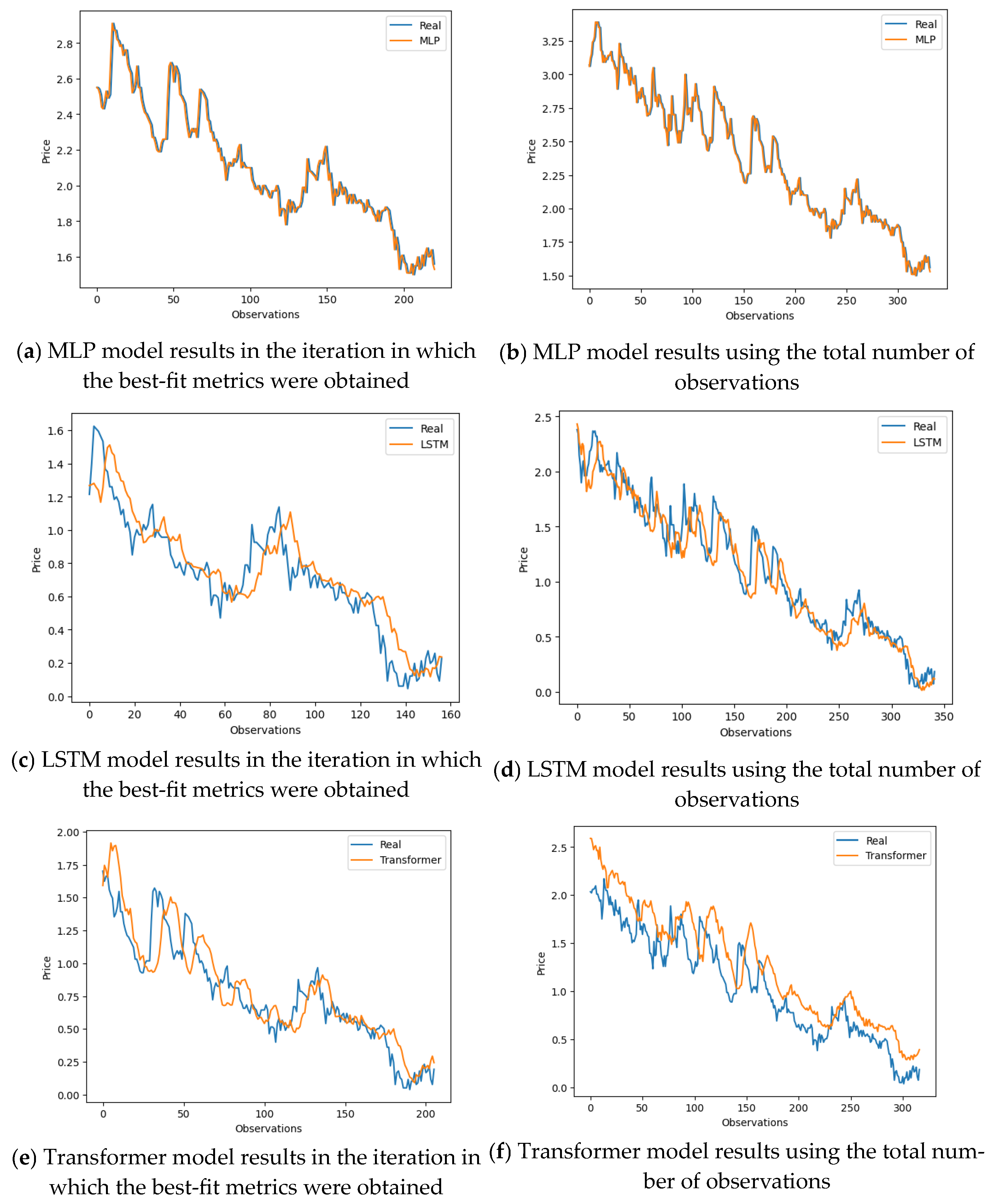
5. Experimental Results

Table 3, Table 4, Table 5 and Table 6 show the results of the methodology applied to the four data series considered in the study. The results illustrate how the last dataset, with the total number of observations, is not the one that achieves the best results on all occasions.
The GOLD time series (Table 3), being the one that consists of the fewest observations, shows that in the first iterations, it already obtains the most accurate results and with the least error.
Table 4 shows the time series related to the data OMIE and it achieves the best results in the first iteration, being the time series that consists of more observations, which shows that it is not necessary to use all of these for the training to be optimal.
The time series with Apple prices (Table 5) shows a greater error as more observations are included. This is because, being a time series with an upward trend, it struggles to accurately model future behavior, leading to worse results as more historical data are used for training.
However, the oil price (Table 6) does show better behavior by including a greater amount of data in the training, being a time series with little marked trend.
The results show how the best metrics are not always obtained in the last iteration with the complete dataset, varying depending on the time series and the model used.
For the time series of WTI oil prices, since the best results have been obtained for the MLP and Transformer ANNs in the last iteration, a comparison has been made with the iterations that have obtained the best metrics in second place, with the fifth being and fourth respectively. The error metrics show a variation of less than 1%; however, the computing time between iterations, which must include 1000 more training observations in the case of this series, does represent a notable difference. In the Apple time series for the MLP model, the sixth iteration, with the lowest error, has been compared with the fourth, the second with the lowest error.
The results tables also show the time needed for training in each of the cases, showing how this methodology can lead to significant savings in computing time by not using all the observations in all cases.

6. Discussion

The results demonstrate that in neural networks, optimal performance is not necessarily tied to the volume of observations in the training set. The findings reveal that the best error metrics vary across different iterations, depending on the characteristics of each time series, indicating that more data does not universally enhance model accuracy. This aligns with previous studies, which suggest that after a certain threshold, adding additional observations does not yield significant improvements in predictive accuracy and may even lead to diminishing returns. Unlike research focused on sparse datasets, where adding synthetic data often helps mitigate high error metrics (as shown by [74,75]), this study highlights that when sufficient data are available, the inclusion of extra observations can sometimes increase error rather than reduce it. This finding challenges the assumption that increasing data volume always enhances model performance, especially for datasets with complex, non-linear temporal dependencies.
The current literature reflects no clear consensus on the ideal quantity of observations for training time series models [76,77,78]. While some studies advocate for larger datasets, others, such as [79,80], report that increasing the number of observations does not necessarily improve error metrics, resonating with the findings. This study adds to this discussion by showing that after a certain threshold, additional data points may not reduce error and, in some cases, may even degrade performance. This pattern is consistent with research by [81], who observed that after reaching a certain number of observations, the error metrics plateaued while computational costs continued to rise. Thus, the results suggest that the relationship between dataset size and neural network performance is non-linear, and that excessive data may impose additional computational burdens without corresponding accuracy gains.
Another important implication of the findings is the potential to enhance computational efficiency. The observation that error rates do not decrease significantly after a certain dataset size suggests that training times could be reduced without compromising model accuracy. This has practical value for applications requiring real-time predictions or those operating under limited computational resources, as it supports the notion that an optimal subset of observations can achieve near-maximum performance while reducing training costs. Such optimization could be particularly beneficial in large-scale prediction systems, where resource allocation and training efficiency are critical factors. By identifying an optimal balance between data volume and accuracy, the approach provides a framework to refine both predictive performance and associated computational expenses.
In a broader context, these findings offer practical guidelines for handling time series prediction problems across various domains, such as finance, healthcare, and environmental forecasting, where data may either be abundant or constrained by factors like data privacy or collection limitations. By leveraging an optimal subset of observations, practitioners can achieve competitive model performance while minimizing computational costs, which is particularly advantageous in real-time forecasting and low-resource environments. Additionally, this approach allows for more sustainable model deployment by reducing energy consumption associated with training on excessive data. As a result, the methodology contributes to a more efficient, scalable approach to time series forecasting that can be tailored to the specific data availability and computational constraints of diverse applications.
Nonetheless, it is important to acknowledge certain limitations of this study. First, the observed behavior varied depending on the specific time series and neural network model employed. This variability means that a single, universal pattern could not be established where a specific iteration or data volume consistently provided the best results across all cases. Consequently, the model developed focuses on identifying the ideal proportion of the training set for each unique application, rather than proposing a one-size-fits-all solution. Future research could benefit from exploring these findings across a broader range of time series types and neural network architectures to better understand how generalizable this approach may be and to refine methods for optimizing training data in neural network-based time series forecasting.

7. Conclusions

The results of this research allow us to conclude that, contrary to what is commonly assumed, a greater number of observations does not necessarily guarantee an improvement in error metrics when training recurrent neural networks, such as MLPs, LSTMs, and transformers, for time series prediction. The best metrics were obtained at different stages of the iterations, depending on the specific characteristics of each series, indicating that the optimal number of observations varies from case to case.
In addition, no evidence of a significant improvement has been found when including more training data in terms of predictive performance, causing in some of the series a significant worsening of the resulting metrics, even leading to an underfitting of the model. This methodology allows significant computational savings by identifying the ideal amount of data for training and excessive training time. Furthermore, the metrics calculated for the training and testing partitions demonstrate that the methodology avoids both underfitting and overfitting.
The practical implications of these findings are significant: it is possible to reduce the number of observations used to train neural networks without losing precision in the predictions, which could optimize training time and reduce the computational resources required. This has a direct impact on the development of real-time forecasting systems or in environments where resources are limited.
Finally, the future implications of this research suggest that it is necessary to develop more accurate techniques to automatically determine the optimal number of observations based on the specific characteristics of the time series and the model used. Reducing redundant or irrelevant data without sacrificing accuracy is a key area for further research.

Author Contributions

Conceptualization, A.L., P.H. and J.E.S.; methodology, A.L.; software, A.L.; validation, A.L.; investigation, A.L., P.H. and J.E.S.; resources, A.L., P.H. and J.E.S.; data curation, A.L., P.H. and J.E.S.; writing—original draft preparation, A.L., P.H. and J.E.S.; writing—review and editing, A.L., P.H. and J.E.S.; visualization, A.L., P.H. and J.E.S.; supervision, A.L., P.H. and J.E.S.; project administration, A.L., P.H. and J.E.S. All authors have read and agreed to the published version of the manuscript.

Funding

This research received no external funding.

Institutional Review Board Statement

Not applicable.

Informed Consent Statement

Not applicable.

Data Availability Statement

Restrictions apply to the availability of these data. Data were obtained from Thomson Eikon Reuters and are available from the Refinitiv application with the permission of Thomson Eikon Reuters. Code Available at: https://colab.research.google.com/drive/1j5p8SRFrIHfz7dPhCwV1dYfetLKYnsUP?usp=sharing (accessed on 19 May 2024).

Conflicts of Interest

The authors declare no conflict of interest.

References

  1. Shiblee, M.; Kalra, P.K.; Chandra, B. Time Series Prediction with Multilayer Perceptron (MLP): A New Generalized Error Based Approach. In Advances in Neuro-Information Processing; Köppen, M., Kasabov, N., Coghill, G., Eds.; Springer: Berlin/Heidelberg, Germany, 2009; pp. 37–44. [Google Scholar]
  2. Yulita, I.N.; Abdullah, A.S.; Helen, A.; Hadi, S.; Sholahuddin, A.; Rejito, J. Comparison multi-layer perceptron and linear regression for time series prediction of novel coronavirus COVID-19 data in West Java. J. Phys. Conf. Ser. 2021, 1722, 012021. [Google Scholar] [CrossRef]
  3. Borghi, P.H.; Zakordonets, O.; Teixeira, J.P. A COVID-19 time series forecasting model based on MLP ANN. Procedia Comput. Sci. 2021, 181, 940–947. [Google Scholar] [CrossRef] [PubMed]
  4. Khashei, M.; Hajirahimi, Z. A comparative study of series arima/mlp hybrid models for stock price forecasting. Commun. Stat. Simul. Comput. 2019, 48, 2625–2640. [Google Scholar] [CrossRef]
  5. Wang, J.; Li, X.; Li, J.; Sun, Q.; Wang, H. NGCU: A New RNN Model for Time-Series Data Prediction. Big Data Res. 2022, 27, 100296. [Google Scholar] [CrossRef]
  6. Amalou, I.; Mouhni, N.; Abdali, A. Multivariate time series prediction by RNN architectures for energy consumption forecasting. Energy Rep. 2022, 8, 1084–1091. [Google Scholar] [CrossRef]
  7. De Rojas, A.L.; Jaramillo-Morán, M.A.; Sandubete, J.E. EMDFormer model for time series forecasting. AIMS Math. 2024, 9, 9419–9434. [Google Scholar] [CrossRef]
  8. Tuli, S.; Casale, G.; Jennings, N.R. TranAD: Deep transformer networks for anomaly detection in multivariate time series data. Proc. VLDB Endow. 2022, 15, 1201–1214. [Google Scholar] [CrossRef]
  9. Brown, T.; Mann, B.; Ryder, N.; Subbiah, M.; Kaplan, J.D.; Dhariwal, P.; Neelakantan, A.; Shyam, P.; Sastry, G.; Askell, A.; et al. Language Models are Few-Shot Learners. In Advances in Neural Information Processing Systems; Curran Associates Inc.: Red Hook, NY, USA, 2020; Volume 33, pp. 1877–1901. [Google Scholar]
  10. Valiant, L.G. A theory of the learnable. Commun. ACM 1984, 27, 1134–1142. [Google Scholar] [CrossRef]
  11. Rivasplata, O.; Parrado-Hernandez, E.; Shawe-Taylor, J.S.; Sun, S.; Szepesvari, C. PAC-Bayes bounds for stable algorithms with instance-dependent priors. In Advances in Neural Information Processing Systems; Curran Associates Inc.: Red Hook, NY, USA, 2018; Volume 31. [Google Scholar]
  12. Xu, P.; Kumar, D.; Yang, W.; Zi, W.; Tang, K.; Huang, C.; Cheung, J.C.K.; Prince, S.J.D.; Cao, Y. Optimizing Deeper Transformers on Small Datasets. In Proceedings of the 59th Annual Meeting of the Association for Computational Linguistics and the 11th International Joint Conference on Natural Language Processing, Online, 1–6 August 2021; Zong, C., Xia, F., Li, W., Navigli, R., Eds.; Association for Computational Linguistics: Stroudsburg, PA, USA, 2021; pp. 2089–2102. [Google Scholar] [CrossRef]
  13. Clark, T.E.; McCracken, M.W. Improving Forecast Accuracy by Combining Recursive and Rolling Forecasts. Int. Econ. Rev. 2009, 50, 363–395. [Google Scholar] [CrossRef]
  14. Stock, J.H.; Watson, M.W. An Empirical Comparison of Methods for Forecasting Using Many Predictors; Princeton University: Princeton, NJ, USA, 2005; Volume 46. [Google Scholar]
  15. Kaveh, M.; Mesgari, M.S. Application of Meta-Heuristic Algorithms for Training Neural Networks and Deep Learning Architectures: A Comprehensive Review. Neural Process. Lett. 2023, 55, 4519–4622. [Google Scholar] [CrossRef]
  16. Zito, F.; Cutello, V.; Pavone, M. Deep Learning and Metaheuristic for Multivariate Time-Series Forecasting. In Proceedings of the 18th International Conference on Soft Computing Models in Industrial and Environmental Applications (SOCO 2023), Salamanca, Spain, 5–7 September 2023; García Bringas, P., Pérez García, H., Martínez de Pisón, F.J., Martínez Álvarez, F., Troncoso Lora, A., Herrero, Á., Calvo Rolle, J.L., Quintián, H., et al., Eds.; Springer Nature: Cham, Switzerland, 2023; pp. 249–258. [Google Scholar]
  17. Mizdrakovic, V.; Kljajic, M.; Zivkovic, M.; Bacanin, N.; Jovanovic, L.; Deveci, M.; Pedrycz, W. Forecasting bitcoin: Decomposition aided long short-term memory based time series modeling and its explanation with Shapley values. Knowl. Based Syst. 2024, 299, 112026. [Google Scholar] [CrossRef]
  18. Adnan, R.M.; Mirboluki, A.; Mehraein, M.; Malik, A.; Heddam, S.; Kisi, O. Improved prediction of monthly streamflow in a mountainous region by Metaheuristic-Enhanced deep learning and machine learning models using hydroclimatic data. Theor. Appl. Climatol. 2024, 155, 205–228. [Google Scholar] [CrossRef]
  19. Zhang, G.; Patuwo, B.E.; Hu, M.Y. Forecasting with artificial neural networks: The state of the art. Int. J. Forecast. 1998, 14, 35–62. [Google Scholar] [CrossRef]
  20. Hochreiter, S.; Schmidhuber, J. Long Short-Term Memory. Neural Comput. 1997, 9, 1735–1780. [Google Scholar] [CrossRef]
  21. Gers, F.A.; Schmidhuber, J.; Cummins, F. Learning to Forget: Continual Prediction with LSTM. Neural Comput. 2000, 12, 2451–2471. [Google Scholar] [CrossRef]
  22. Malhotra, P.; Vig, L.; Shroff, G.; Agarwal, P. Long short term memory networks for anomaly detection in time series. In Proceedings of the 23rd European Symposium on Artificial Neural Networks, Computational Intelligence and Machine Learning, ESANN, Bruges, Belgium, 4–6 October 2015; Volume 2015, p. 89. [Google Scholar]
  23. Guo, T.; Lin, T.; Lu, Y. An interpretable LSTM neural network for autoregressive exogenous model. arXiv 2018, arXiv:1804.05251. [Google Scholar]
  24. Siami-Namini, S.; Tavakoli, N.; Namin, A.S. The Performance of LSTM and BiLSTM in Forecasting Time Series. In Proceedings of the 2019 IEEE International Conference on Big Data (Big Data), Los Angeles, CA, USA, 9–12 December 2019; pp. 3285–3292. [Google Scholar]
  25. Zhang, T.; Zhang, Y.; Cao, W.; Bian, J.; Yi, X.; Zheng, S.; Li, J. Less Is More: Fast Multivariate Time Series Forecasting with Light Sampling-oriented MLP Structures. arXiv 2022. [Google Scholar] [CrossRef]
  26. Yi, K.; Zhang, Q.; Fan, W.; Wang, S.; Wang, P.; He, H.; An, N.; Lian, D.; Cao, L.; Niu, Z. Frequency-domain MLPs are More Effective Learners in Time Series Forecasting. Adv. Neural Inf. Process. Syst. 2023, 36, 76656–76679. [Google Scholar]
  27. Madhusudhanan, K.; Jawed, S.; Schmidt-Thieme, L. Hyperparameter Tuning MLPs for Probabilistic Time Series Forecasting. arXiv 2024. [Google Scholar] [CrossRef]
  28. Lazcano, A.; Jaramillo-Morán, M.A.; Sandubete, J.E. Back to Basics: The Power of the Multilayer Perceptron in Financial Time Series Forecasting. Mathematics 2024, 12, 1920. [Google Scholar] [CrossRef]
  29. Salinas, D.; Flunkert, V.; Gasthaus, J.; Januschowski, T. DeepAR: Probabilistic forecasting with autoregressive recurrent networks. Int. J. Forecast. 2020, 36, 1181–1191. [Google Scholar] [CrossRef]
  30. Lai, G.; Chang, W.-C.; Yang, Y.; Liu, H. Modeling Long-and Short-Term Temporal Patterns with Deep Neural Networks. In Proceedings of the 41st International ACM SIGIR Conference on Research and Development in Information Retrieval, Ann Arbor, MI, USA, 8–12 July 2018; pp. 95–104. [Google Scholar]
  31. Cheng, B.; Titterington, D.M. Neural Networks: A Review from a Statistical Perspective. Stat. Sci. 1994, 9, 2–30. [Google Scholar]
  32. Kim, K.; Han, I. Genetic algorithms approach to feature discretization in artificial neural networks for the prediction of stock price index. Expert Syst. Appl. 2000, 19, 125–132. [Google Scholar] [CrossRef]
  33. Weiss, K.; Khoshgoftaar, T.M.; Wang, D. A survey of transfer learning. J. Big Data 2016, 3, 9. [Google Scholar] [CrossRef]
  34. Dridi, A.; Afifi, H.; Moungla, H.; Boucetta, C. Transfer Learning for Classification and Prediction of Time Series for Next Generation Networks. In Proceedings of the ICC 2021—IEEE International Conference on Communications, Montreal, QC, Canada, 14–18 June 2021; pp. 1–6. [Google Scholar]
  35. Oreshkin, B.; Carpo, D.; Chapados, N.; Bengio, Y. N-BEATS: Neural basis expansion analysis for interpretable time series forecasting. arXiv 2019, arXiv:1905.10437. [Google Scholar]
  36. Ruder, S. An Overview of Multi-Task Learning in Deep Neural Networks. arXiv 2017, arXiv:1706.05098. [Google Scholar]
  37. Mahmoud, R.A.; Hajj, H.; Karameh, F.N. A systematic approach to multi-task learning from time-series data. Appl. Soft Comput. 2020, 96, 106586. [Google Scholar] [CrossRef]
  38. Abolghasemi, M.; Hyndman, R.; Spiliotis, E.; Bergmeir, C. Model selection in reconciling hierarchical time series. Mach. Learn. 2022, 111, 739–789. [Google Scholar] [CrossRef]
  39. Hyndman, R.J.; Koehler, A.B. Another look at measures of forecast accuracy. Int. J. Forecast. 2006, 22, 679–688. [Google Scholar] [CrossRef]
  40. Cerqueira, V.; Torgo, L.; Smailović, J.; Mozetič, I. A Comparative Study of Performance Estimation Methods for Time Series Forecasting. In Proceedings of the 2017 IEEE International Conference on Data Science and Advanced Analytics (DSAA), Tokyo, Japan, 19–21 October 2017; pp. 529–538. [Google Scholar]
  41. Inoue, A.; Jin, L.; Rossi, B. Rolling window selection for out-of-sample forecasting with time-varying parameters. J. Econom. 2017, 196, 55–67. [Google Scholar] [CrossRef]
  42. Casolaro, A.; Capone, V.; Iannuzzo, G.; Camastra, F. Deep Learning for Time Series Forecasting: Advances and Open Problems. Information 2023, 14, 598. [Google Scholar] [CrossRef]
  43. Zivot, E.; Wang, J. Rolling Analysis of Time Series. In Modeling Financial Time Series with S-Plus®; Zivot, E., Wang, J., Eds.; Springer: New York, NY, USA, 2003; pp. 299–346. ISBN 978-0-387-21763-5. [Google Scholar]
  44. Moghaddam, A.H.; Moghaddam, M.H.; Esfandyari, M. Stock market index prediction using artificial neural network. J. Econ. Finance Adm. Sci. 2016, 21, 89–93. [Google Scholar] [CrossRef]
  45. Göçken, M.; Özçalıcı, M.; Boru, A.; Dosdoğru, A.T. Integrating metaheuristics and Artificial Neural Networks for improved stock price prediction. Expert Syst. Appl. 2016, 44, 320–331. [Google Scholar] [CrossRef]
  46. Keles, D.; Scelle, J.; Paraschiv, F.; Fichtner, W. Extended forecast methods for day-ahead electricity spot prices applying artificial neural networks. Appl. Energy 2016, 162, 218–230. [Google Scholar] [CrossRef]
  47. Fan, X.; Li, S.; Tian, L. Chaotic characteristic identification for carbon price and an multi-layer perceptron network prediction model. Expert Syst. Appl. 2015, 42, 3945–3952. [Google Scholar] [CrossRef]
  48. Han, M.; Ding, L.; Zhao, X.; Kang, W. Forecasting carbon prices in the Shenzhen market, China: The role of mixed-frequency factors. Energy 2019, 171, 69–76. [Google Scholar] [CrossRef]
  49. Li, W. Analysis on the Weight initialization Problem in Fully-Connected Multi-layer Perceptron Neural Network. In Proceedings of the 2020 International Conference on Artificial Intelligence and Computer Engineering (ICAICE), Beijing, China, 6–8 November 2020; pp. 150–153. [Google Scholar]
  50. Zhang, A.; Lipton, Z.C.; Li, M.; Smola, A.J. Dive into Deep Learning. arXiv 2021, arXiv:2106.11342. [Google Scholar]
  51. Devlin, J.; Chang, M.-W.; Lee, K.; Toutanova, K. BERT: Pre-training of Deep Bidirectional Transformers for Language Understanding. arXiv 2019. [Google Scholar] [CrossRef]
  52. Dosovitskiy, A.; Beyer, L.; Kolesnikov, A.; Weissenborn, D.; Zhai, X.; Unterthiner, T.; Dehghani, M.; Minderer, M.; Heigold, G.; Gelly, S.; et al. An Image is Worth 16x16 Words: Transformers for Image Recognition at Scale. arXiv 2021. [Google Scholar] [CrossRef]
  53. Cholakov, R.; Kolev, T. Transformers predicting the future. Applying attention in next-frame and time series forecasting. arXiv 2021. [Google Scholar] [CrossRef]
  54. Lim, B.; Arık, S.Ö.; Loeff, N.; Pfister, T. Temporal Fusion Transformers for interpretable multi-horizon time series forecasting. Int. J. Forecast. 2021, 37, 1748–1764. [Google Scholar] [CrossRef]
  55. Wu, H.; Xu, J.; Wang, J.; Long, M. Autoformer: Decomposition Transformers with Auto-Correlation for Long-Term Series Forecasting. In Advances in Neural Information Processing Systems; Curran Associates Inc.: Red Hook, NY, USA, 2021; Volume 34, pp. 22419–22430. [Google Scholar]
  56. Zeyer, A.; Bahar, P.; Irie, K.; Schlüter, R.; Ney, H. A Comparison of Transformer and LSTM Encoder Decoder Models for ASR. In Proceedings of the 2019 IEEE Automatic Speech Recognition and Understanding Workshop (ASRU), Singapore, 4–18 December 2019; pp. 8–15. [Google Scholar]
  57. Vaswani, A.; Shazeer, N.; Parmar, N.; Uszkoreit, J.; Jones, L.; Gomez, A.N.; Kaiser, Ł.; Polosukhin, I. Attention is All you Need. In Advances in Neural Information Processing Systems; Curran Associates Inc.: Red Hook, NY, USA, 2017; Volume 30. [Google Scholar]
  58. Dauphin, Y.N.; Bengio, Y. Big Neural Networks Waste Capacity. arXiv 2013. [Google Scholar] [CrossRef]
  59. Botchkarev, A. Performance Metrics (Error Measures) in Machine Learning Regression, Forecasting and Prognostics: Properties and Typology. arXiv 2018, arXiv:1809.03006. [Google Scholar]
  60. Olawoyin, A.; Chen, Y. Predicting the Future with Artificial Neural Network. Procedia Comput. Sci. 2018, 140, 383–392. [Google Scholar] [CrossRef]
  61. Li, J. Assessing the accuracy of predictive models for numerical data: Not r nor r2, why not? Then what? PLoS ONE 2017, 12, e0183250. [Google Scholar] [CrossRef]
  62. Botchkarev, A. A new typology design of performance metrics to measure errors in machine learning regression algorithms. Interdiscip. J. Inf. Knowl. Manag. 2019, 14, 45–76. [Google Scholar] [CrossRef]
  63. Nakagawa, S.; Schielzeth, H. A general and simple method for obtaining R2 from generalized linear mixed-effects models. Methods Ecol. Evol. 2013, 4, 133–142. [Google Scholar] [CrossRef]
  64. Chicco, D.; Warrens, M.J.; Jurman, G. The coefficient of determination R-squared is more informative than SMAPE, MAE, MAPE, MSE and RMSE in regression analysis evaluation. PeerJ Comput. Sci. 2021, 7, e623. [Google Scholar] [CrossRef]
  65. Naser, M.Z.; Alavi, A.H. Error Metrics and Performance Fitness Indicators for Artificial Intelligence and Machine Learning in Engineering and Sciences. Archit. Struct. Constr. 2023, 3, 499–517. [Google Scholar] [CrossRef]
  66. Lin, T.; Guo, T.; Aberer, K. Hybrid Neural Networks for Learning the Trend in Time Series. In Proceedings of the Twenty-Sixth International Joint Conference on Artificial Intelligence, Melbourne, Australia, 19–25 August 2017; pp. 2273–2279. [Google Scholar] [CrossRef]
  67. Ouma, Y.O.; Cheruyot, R.; Wachera, A.N. Rainfall and runoff time-series trend analysis using LSTM recurrent neural network and wavelet neural network with satellite-based meteorological data: Case study of Nzoia hydrologic basin. Complex Intell. Syst. 2022, 8, 213–236. [Google Scholar] [CrossRef]
  68. Zhang, G.P.; Kline, D.M. Quarterly Time-Series Forecasting with Neural Networks. IEEE Trans. Neural Netw. 2007, 18, 1800–1814. [Google Scholar] [CrossRef]
  69. Sun, R. Optimization for deep learning: Theory and algorithms. arXiv 2019. [Google Scholar] [CrossRef]
  70. Hanifi, S.; Cammarono, A.; Zare-Behtash, H. Advanced hyperparameter optimization of deep learning models for wind power prediction. Renew. Energy 2024, 221, 119700. [Google Scholar] [CrossRef]
  71. Goodfellow, I.; Pouget-Abadie, J.; Mirza, M.; Xu, B.; Warde-Farley, D.; Ozair, S.; Courville, A.; Bengio, Y. Generative adversarial networks. Commun. ACM 2020, 63, 139–144. [Google Scholar] [CrossRef]
  72. Beck, J.V.; Arnold, K.J. Parameter Estimation in Engineering and Science; John and Wiley and Sons: Hoboken, NJ, USA, 1977; ISBN 978-0-471-06118-2. [Google Scholar]
  73. Smith, L.N. Cyclical Learning Rates for Training Neural Networks. In Proceedings of the 2017 IEEE Winter Conference on Applications of Computer Vision (WACV), Santa Rosa, CA, USA, 24–31 March 2017; pp. 464–472. [Google Scholar]
  74. Bandara, K.; Hewamalage, H.; Liu, Y.-H.; Kang, Y.; Bergmeir, C. Improving the accuracy of global forecasting models using time series data augmentation. Pattern Recognit. 2021, 120, 108148. [Google Scholar] [CrossRef]
  75. Iglesias, G.; Talavera, E.; González-Prieto, Á.; Mozo, A.; Gómez-Canaval, S. Data Augmentation techniques in time series domain: A survey and taxonomy. Neural Comput. Appl. 2023, 35, 10123–10145. [Google Scholar] [CrossRef]
  76. Haussler, D. Decision theoretic generalizations of the PAC model for neural net and other learning applications. Inf. Comput. 1992, 100, 78–150. [Google Scholar] [CrossRef]
  77. Meade, N. Evidence for the selection of forecasting methods. J. Forecast. 2000, 19, 515–535. [Google Scholar] [CrossRef]
  78. Shi, J.; Ma, Q.; Ma, H.; Li, L. Scaling Law for Time Series Forecasting. arXiv 2024. [Google Scholar] [CrossRef]
  79. Guo, Z.X.; Wong, W.K.; Li, M. Sparsely connected neural network-based time series forecasting. Inf. Sci. 2012, 193, 54–71. [Google Scholar] [CrossRef]
  80. Linjordet, T.; Balog, K. Impact of Training Dataset Size on Neural Answer Selection Models. In Advances in Information Retrieval; Azzopardi, L., Stein, B., Fuhr, N., Mayr, P., Hauff, C., Hiemstra, D., Eds.; Springer International Publishing: Cham, Switzerland, 2019; pp. 828–835. [Google Scholar]
  81. Zhou, J.; Shi, J.; Li, G. Fine tuning support vector machines for short-term wind speed forecasting. Energy Convers. Manag. 2011, 52, 1990–1998. [Google Scholar] [CrossRef]
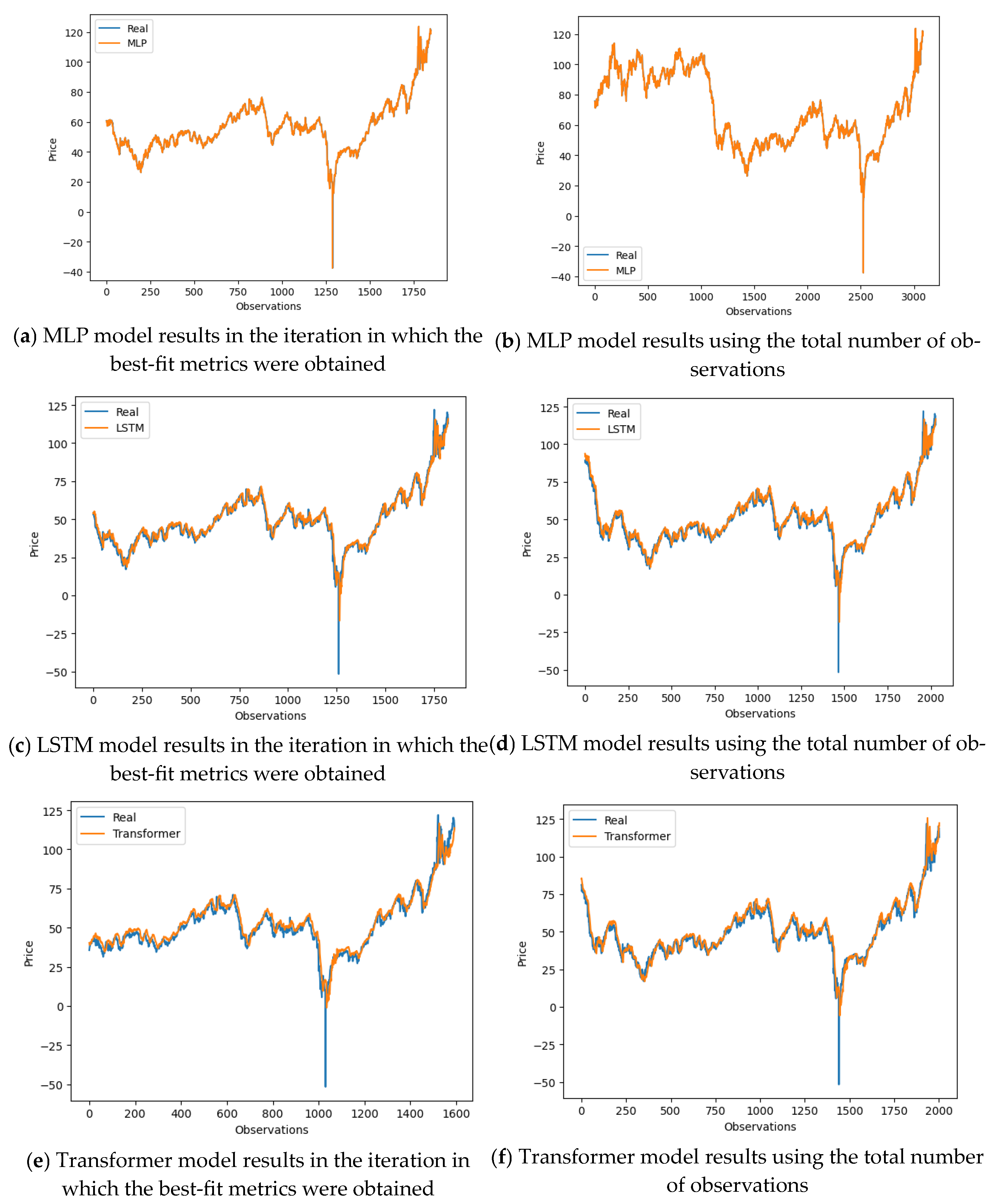
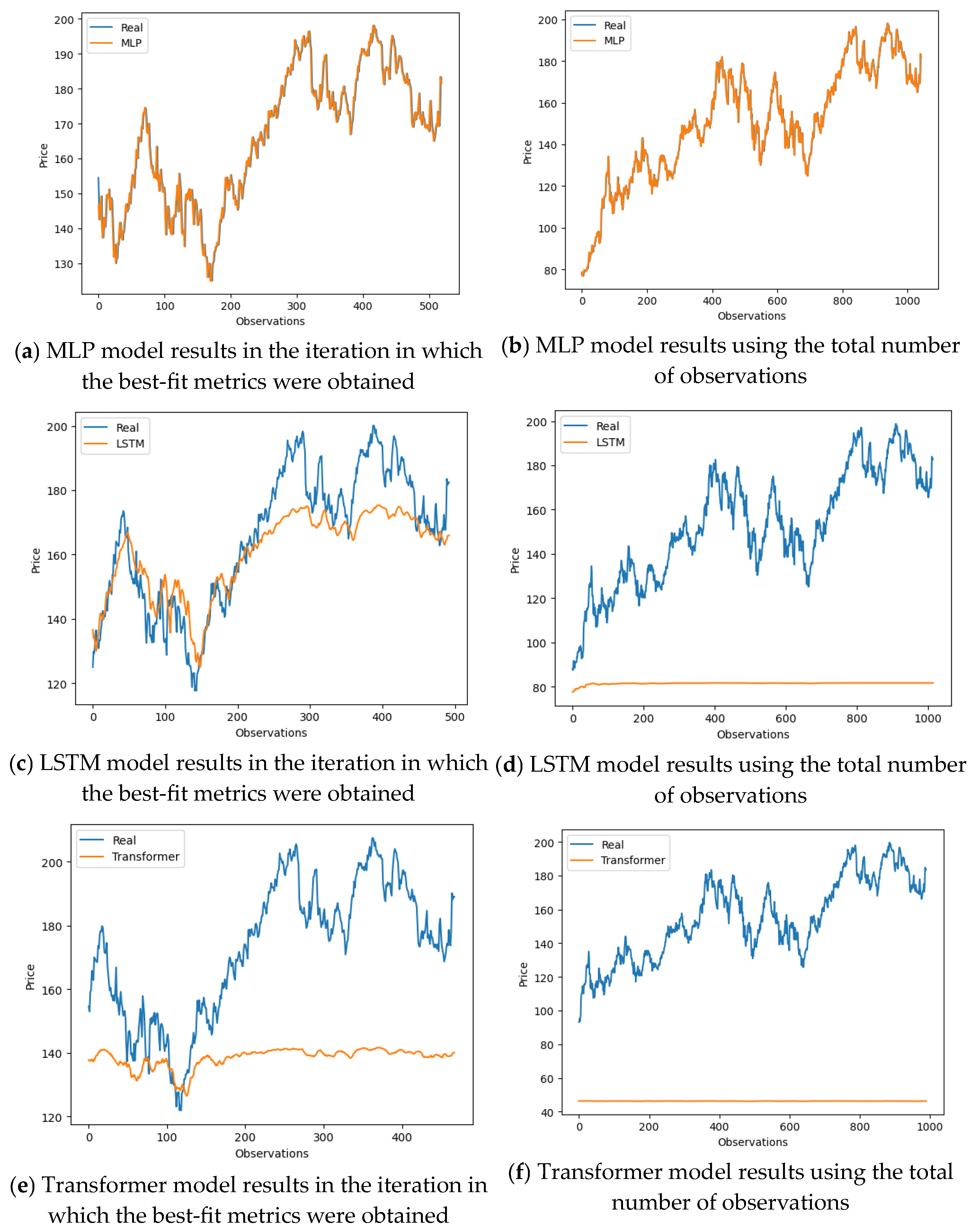
Figure 1. LSTM neural network.
Applsci 14 11081 g001
Figure 2. Transformer neural network.
Applsci 14 11081 g002
Figure 3. Walking back.
Applsci 14 11081 g003
Figure 4. Gold results.
Applsci 14 11081 g004
Figure 5. WTI results.
Applsci 14 11081 g005
Figure 6. Apple results.
Applsci 14 11081 g006
Figure 7. OMIE results.
Applsci 14 11081 g007
Table 1. Dataset division.
Time Serie1st Iteration2nd Iteration3rd Iteration4th Iteration5th Iteration6th IterationTotal
Observations
TrainTestTrainTestTrainTestTrainTestTrainTestTrainTest
GOLD74018688822310362601184297133233414803711851
WTI41151029493812355761144165841647740818528230205810,288
Apple20885222505627292373133408363758940417510445219
OMIE16,612415319,380484622,149553824,918623027,686692227,686692234,608
Table 2. Parameters selected.
ModelLearning RateBatchEpochHidden LayersOptimizerFf_dimNum_heads
Transformer0.0011501501Adam756
LSTM0.001251002Adam--
MLP0.00125752Adam--
Table 3. GOLD results.
Metrics GOLD
Time SerieANNRMSEMSEMAPER2Time
MLP0.080.0115.470.956.37
0.060.0018.360.976.86
0.070.0120.090.966.27
0.070.0021.670.977.86
0.070.0024.140.977.09
0.100.0126.470.968.96
LSTM0.150.0232.740.8026.07
0.160.0234.130.7932.11
0.180.0327.210.8430.14
0.180.0325.060.8532.36
0.180.0326.000.8734.34
0.180.0317.820.9140.57
TRANS3.6913.641101.49−169.9031.65
0.230.0559.720.4834.93
0.190.0331.230.7640.77
0.300.0931.930.5954.46
0.240.0532.900.7560.89
0.290.0847.880.7061.07
Table 4. WTI results.
Metrics WTI
Time SerieANNRMSEMSEMAPER2Time
MLP2.496.2041.580.9716.62
2.345.4537.210.9716.47
2.305.2835.030.9817.66
2.174.7234.630.9820.33
2.024.0735.060.9829.40
2.014.0235.630.9831.85
LSTM5.3528.6943.110.9570.63
4.5620.818.890.9472.87
4.3719.178.470.94110.60
4.0416.337.510.95118.62
4.0316.297.880.95131.19
4.1517.298.050.94151.46
TRANS6.8747.3245.970.92138.38
5.1927.029.800.93217.77
5.1626.699.870.92216.02
4.7822.909.160.93223.83
5.0025.009.510.92264.62
4.6021.198.610.93300.67
Table 5. Apple results.
Metrics Apple
Time SerieANNRMSEMSEMAPER2Time
MLP2.757.5513.410.989.22
3.089.5112.340.9710.49
3.8714.9712.310.9711.34
2.827.9714.720.9813.45
3.5512.6016.640.9815.65
2.727.4022.220.9915.34
LSTM11.08122.895.200.7142.09
17.81317.189.150.0044.47
27.19739.2913.75−1.4461.23
28.99840.8914.47−1.3170.45
36.041299.1519.15−1.9067.74
75.275666.9045.01−8.0080.35
TRANS38.861510.4818.79−2.36113.49
48.002304.4427.09−5.96121.31
86.167424.2450.37−23.44146.48
108.1011,685.8564.97−32.37142.26
104.3810,896.0963.74−24.72194.40
111.0312,329.7069.36−21.07207.48
Table 6. OMIE results.
Metrics OMIE
Time SerieANNRMSEMSER2Time
MLP10.71114.730.8435.81
11.02121.550.8664.83
12.02144.360.8561.99
12.95167.580.8559.95
12.71161.470.8770.77
12.91166.650.8871.21
LSTM16.54273.870.63254.31
16.85284.110.67267.75
18.62346.750.64308.86
19.78391.530.66413.56
19.02361.810.71422.07
20.35414.430.71436.84
TRANS16.71279.280.63686.82
17.19295.690.65829.67
18.52343.010.64880.48
19.64385.830.66997.92
18.73351.080.721130.10
21.47461.040.671150.56
Disclaimer/Publisher’s Note: The statements, opinions and data contained in all publications are solely those of the individual author(s) and contributor(s) and not of MDPI and/or the editor(s). MDPI and/or the editor(s) disclaim responsibility for any injury to people or property resulting from any ideas, methods, instructions or products referred to in the content.

