RADH-A Reversible and Authenticable Data Hiding Scheme in Encrypted Domain Based on Image Interpolation and Substitution

Abstract

The rise of the Internet has transformed communication and information access, but it also raises serious privacy concerns, especially regarding personal image sharing. This paper presents a novel reversible and authenticable data-hiding scheme for encrypted images that utilizes interpolation techniques and substitution methods. Our encryption system achieves a lower correlation among neighboring pixels, ensuring a more uniform distribution in the encrypted image. The stego images do not reveal any information about the original cover image or secret data. The embedded authentication data provides the ability to verify the authenticity of the image and localize the tampering. Experimental results show that our scheme can securely protect an image from unauthorized access and verify its authenticity.

1. Introduction

The widespread adoption of the Internet has transformed nearly every aspect of modern life. With billions of users connected globally, the Internet has become an essential part of daily life, enabling instant communication and access to a vast array of resources. However, with this increase in connectivity comes the growing concern for privacy and secret communication. Data hiding that involves concealing specific information to protect it from unauthorized access or manipulation provides a satisfactory solution for secret communication. Hiding secret data in the cover image has been proposed for a variety of applications, including image copyright protection, annotation, and image authentication.

Inevitably, hiding data in the cover image changes the image content, though the hiding distortion is very low and imperceptible to human eyes. Reversible data hiding (RDH) [1,2,3,4,5,6,7,8,9,10] allows data to be embedded into an image in such a way that both the hidden data and the original image can be fully recovered, which is needed for situations where the integrity of the original image must be preserved after extracting the embedded data. It is especially crucial in fields like medical images, legal documents, and scientific data, where any alteration or distortion of the original data could lead to incorrect interpretations or harmful consequences.

Fridrich et al. [1] introduced a lossless data embedding scheme using a lossless compression algorithm, which compresses bits that are impacted by embedding to reserve space for hiding data. The secret data, along with the compressed bits, are then embedded within the reserved space in the cover image. In 2003, Tian [2] developed a high-capacity reversible data hiding method utilizing a difference expansion (DE) technique, embedding secret data in the pixel differences on high-pass bands of the 1-D Haar wavelet transform. This DE method enables a high bit rate of 0.15 to 1.97 bpp, marking a significant enhancement in hiding capacity. Thodi and Rodriguez [3] later introduced an improved version of the DE scheme, called prediction-error expansion, which leverages local pixel correlations more effectively than DE. Their method demonstrated a doubled maximum hiding capacity compared to DE in the experimental results.

In 2006, Ni et al. [4] introduced a histogram-based reversible data hiding method that uses pairs of peak and zero points to embed data into histogram bins, achieving low embedding distortion. To further enhance hiding capacity, Lin et al. [5] proposed a multilevel reversible data hiding scheme using difference image histogram modification, combining peak-point detection with a multilevel hiding strategy to ensure reversibility while increasing capacity. Tai et al. [6] extended histogram modification by using pixel differences and introduced a binary tree structure to eliminate the need for communicating overhead information to the recipient. Reversible data-hiding techniques have also been explored in the compression domain, including JPEG [7], SMVQ [8], and wavelet domains [9].

Reversible data hiding based on image interpolation [11,12,13,14,15,16,17] has been proposed to ensure both integrity and reversibility of the image. Interpolated images, generated by scaling or resolution enhancement, provide space for data embedding. Chen et al. [12] used various interpolation techniques to create a hiding room, embedding the decimal-converted secret data into cover pixels by adding or subtracting values. Hassan and Gutub [13] employed enhanced neighbor mean interpolation (ENMI) and modified neighbor mean interpolation (MNMI) to scale up images before embedding, improving hiding capacity. A novel two-layer secure scheme [14] combined interpolation-based data hiding with difference expansion, utilizing the maximum pixel difference to provide high-capacity data hiding without compromising image quality. Bai et al. [15] proposed an interpolation-based scheme that selects different functions to compute interpolation values based on secret data.

In scenarios where privacy and sensitive content must be protected, reversible data hiding for encrypted images (RDHEI) [16,18,19,20,21,22,23] securely embeds data within encrypted images, allowing secure storage and transmission. Unauthorized viewers cannot access hidden data without proper decryption, achieving two-layer protection through encryption and data hiding. Zhong et al. [16] used the Arnold matrix to encrypt cover images, embedding secret data into a new image created by an enhanced encrypted image interpolation algorithm. Chen et al. [19] developed an RDHEI model with multiple data-hiders using secret sharing, where the original image is split into encrypted parts and shared among data-hiders; the original image can be restored by collecting enough marked images.

Since finding extra hiding space in encrypted images is challenging due to maximum entropy, some methods [22,23] use interpolation to determine whether a pixel is viable for embedding. In this paper, we propose a high-capacity reversible data-hiding method for encrypted images that enhances privacy protection by employing the Fisher–Yates shuffle algorithm [24] to randomly shuffle pixel sequences. A chaotic sequence diffuses pixels to encrypt the cover image, and interpolation creates space for embedding. In our separate-key strategy, only a receiver with both an encryption key and a data-hiding key can extract secret data and recover the cover image, while a receiver with only the encryption key can only recover the cover image. The method aims to maximize hiding capacity while preserving image integrity and confidentiality.

To make this paper self-contained, Section 2 elaborates on the proposed scheme in detail. Section 3 presents experimental validation, including encryption analysis and performance comparisons with existing reversible data hiding methods. Finally, Section 4 concludes the paper.

2. Proposed Scheme

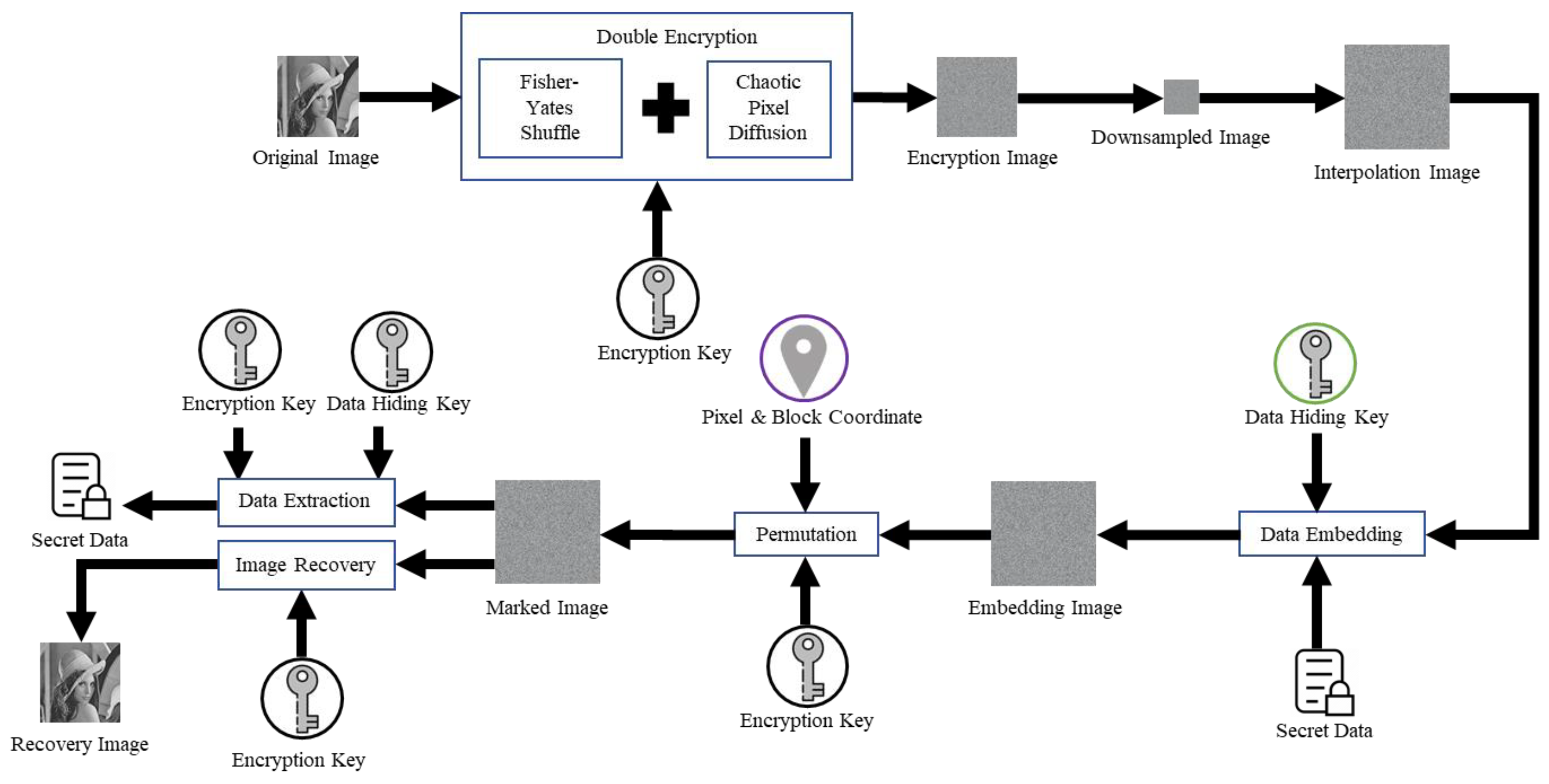
We propose reversible data hiding in encrypted images based on image interpolation for tamper detection. The flowchart of the proposed scheme, which consists of image encryption, image interpolation, data hiding, data extraction, and image recovery, is illustrated in Figure 1. The details of the proposed scheme are described as follows.

2.1. Image Encryption

We introduce a dual encryption technique involving Fisher–Yates shuffle and chaotic pixel diffusion, combining these two encryption methods to enhance the disorderliness of the image, thereby further improving its security and confidentiality. We first represent the original grayscale image sized W × H as a matrix OI. Each pixel in the original image, OI, is shuffled at the 8-bit level within itself. Then, convert the bit-level shuffled image into a one-dimensional vector denoted as S_OI sized as W × H. Next, the Fisher–Yates shuffle algorithm is deployed to shuffle the pixels in a completely random order within the S_OI. Subsequently, the one-dimensional vector S_OI is converted into a two-dimensional matrix OI′. We employ the logistic mapping defined in Equation (1) to generate a one-dimensional chaotic encryption matrix by calculating the next value x′ of x as

x′ = μ × x × (1 − x),

(1)

where x is the initial value for the logistic map, which is used to generate chaotic values and μ is the chaotic parameter. The value range of x must be between 0 and 1, as logistic mapping operates within this domain to maintain its behavior. The parameter μ must be maintained within the range of 3.5699456 ≤ μ ≤ 4 to preserve the chaotic state.

Therefore, a one-dimensional chaotic matrix CH of size W × H can be generated as

CH(i + 1) = μ × CH(i) × (1 − CH(i)),

(2)

where W and H were defined as the width and height of the original image and i is an indicator representing the index in the one-dimensional chaotic matrix CH. It is used to calculate the next value in the sequence using the logistic map formula. It is noted that the value range of i depends on the size of the chaotic matrix, which matches the total number of pixels in the image (i.e., W × H). In other words, i typically ranges from 1 to W × H to iterate through all indices in chaotic matrix CH. x′ is assigned to CH(1). Subsequently, a one-dimensional chaotic matrix CH is converted to the unit8 type as CH₈ = unit8(255 ∗ CH), and then a two-dimensional chaotic encryption matrix ${D_{CH}}_8$ is generated as ${D_{CH}}_8$ = double(reshape(${CH}_8$, W, H)). Finally, a bitwise XOR operation is conducted between matrix O′ and chaotic encryption matrix ${D_{CH}}_8$ to obtain the dual encryption matrix E as

$$E={\mathit{OI}}^{\prime } \oplus {D_{CH}}_8$$

(3)

Here, E also represents the encrypted image. It is noted that the pixel values of grayscale images range from 0 to 255, they are converted to their 8-bit binary representation before performing the XOR operation. For example, a pixel value of 120 in OI′ (binary: 01111000) corresponds to a value of 45 in ${D_{CH}}_8$ (binary: 00101101), and the XOR operation produces a result of 85 (binary: 01010101). It is noted that the same concept can also be extended to color images. Moreover, the proposed framework is highly flexible, allowing the image encryption method to be replaced with other well-known encryption algorithms, such as AES, to meet the user’s requirements. Despite these substitutions, the framework can still work seamlessly with the proposed image interpolation, data hiding, data extraction, and image recovery processes.

2.2. Image Interpolation

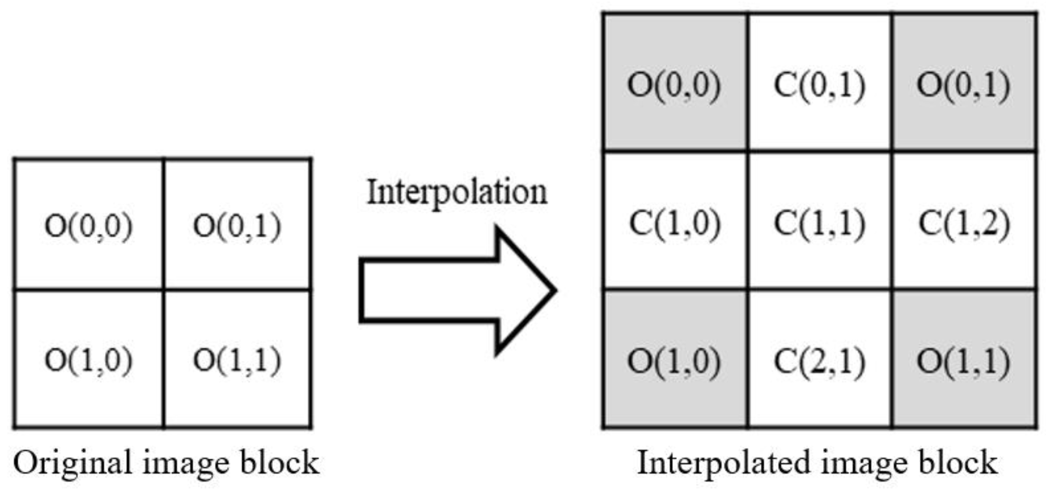
First, the encrypted image E is divided into non-overlapping 2 × 2 blocks. Next, each 2 × 2 block is interpolated to a 3 × 3 interpolated block. Notably, the four original pixels in the 2 × 2 block are rearranged to the four corners of the 3 × 3 interpolated block. The mapping between each 2 × 2 block and its corresponding 3 × 3 interpolated block is illustrated in Figure 2. After all 2 × 2 blocks in the original image have undergone the interpolation operation defined in Equation (4), the final interpolated image C is obtained.

The Nearest Neighbor Mean Interpolation (NMI) technique is applied to generate interpolation image blocks. For boundary pixels, the neighboring pixel values are copied to fill the gap. For internal pixels, the average value of neighboring pixels is used. It is worth noting that in the interpolation image block shown in Figure 2, all original pixels O(0,0), O(0,1), O(1,0) and O(1,1) located in the interpolation image block will not be changed even during the embedding stage, while the interpolated pixels C(0,1), C(1,0), C(1,1), C(1,2), and C(2,1) will be influenced by the embedded secret information. The definitions for the five interpolated pixels are defined as

$$\left\{\begin{array}{c}C\left(0, j\right)={\displaystyle \frac{\left(O\left(0, j-1\right)+ O\left(0, j\right)\right)}{2}}\\ \begin{array}{c}C\left(i, 0\right)={\displaystyle \frac{\left(O\left(i-1, 0\right)+ O\left(i, 0\right)\right)}{2}}\\ \begin{array}{c}C\left(n, j\right)={\displaystyle \frac{\left(O\left(n-1, j-1\right)+ O\left(n-1, j\right)\right)}{2}}\\ C\left(i, m\right)={\displaystyle \frac{\left(O\left(i-1, m-1\right)+ O\left(i, m-1\right)\right)}{2}}\\ C\left(i, j\right)={\displaystyle \frac{\left(O\left(i-1, j-1\right)+ O\left(i-1, j\right)+ O\left(i, j-1\right)+ O\left(i, j\right)\right)}{4}}\end{array}\end{array}\end{array}\right.$$

(4)

For ease of explanation, in the subsequent stages of data hiding and extraction, the four original pixels copied from the 2 × 2 block within the interpolated image block will be uniformly represented as O, while the remaining five interpolated pixels will be uniformly represented as C.

2.3. Data Hiding

For each interpolated image block of 3 × 3 pixels shown in Figure 2, 16-bit secret data are used to be embedded into the four interpolated pixels C(0,1), C(1,0), C(1,2), C(2,1). We embed the 4-bit secret data {b₁, b₂, b₃, b₄} into the four least significant bits (LSBs) of the interpolated pixel within the block by

$$C^{\prime }\left(i, j\right)=16\times \left[{\displaystyle \frac{C\left(i, j\right)}{16}}\right]+8\times b_4+4\times { b}_3+2\times { b}_2+b_1$$

(5)

where C′(i,j)∈{C′(0,1), C′(1,0), C′(1,2), C′(2,1)} is the stego pixel. Moreover, in order to achieve encrypted image authentication, 3-bit authentication data are used to be embedded into the central interpolated pixel C(1, 1) within the block for tamper detection. Note that we use the authentication data to identify any modification made to the authenticated image. The authentication data of the three bits are generated by checking the intensity-relation of each block. For each interpolated image block of 3 × 3 pixels shown in Figure 2, the authentication data are computed by

$$\begin{gathered} a_1=\left\{\begin{array}{c}1,\\ 0,\end{array}\right. \begin{array}{l}\mathrm{i}\mathrm{f} O\left(0, 0\right)<O\left(\mathrm{0,1}\right),\\ \mathrm{o}\mathrm{t}\mathrm{h}\mathrm{e}\mathrm{r}\mathrm{w}\mathrm{i}\mathrm{s}\mathrm{e}.\end{array} \\ {a}_2=\left\{\begin{array}{c}1,\\ 0,\end{array}\right. \begin{array}{l}\mathrm{i}\mathrm{f} O\left(0, 0\right)<O\left(\mathrm{1,0}\right),\\ \mathrm{o}\mathrm{t}\mathrm{h}\mathrm{e}\mathrm{r}\mathrm{w}\mathrm{i}\mathrm{s}\mathrm{e}.\end{array} \\ {a}_3=\left\{\begin{array}{c}1,\\ 0,\end{array}\right. \begin{array}{l}\mathrm{i}\mathrm{f} O\left(0, 0\right)<O\left(\mathrm{1,1}\right),\\ \mathrm{o}\mathrm{t}\mathrm{h}\mathrm{e}\mathrm{r}\mathrm{w}\mathrm{i}\mathrm{s}\mathrm{e}.\end{array} \end{gathered}$$

(6)

where a_i is the authentication data. Then, we embed the 3-bit authentication data {a₁, a₂, a₃} into the three LSBs of the central interpolated pixel C(1,1) within the block by

$$C^{\prime }\left(1, 1\right)=8\times \left[{\displaystyle \frac{C\left(1, 1\right)}{8}}\right]+4\times a_3 +2\times { a}_2+a_1$$

(7)

where C′(1,1) is the stego pixel.

2.4. Data Extraction and Image Recovery

After receiving the encrypted stego image, the pixels located at the corner positions in the 3 × 3 interpolation image block are retrieved to obtain the original 2 × 2 reconstructed encrypted blocks. As long as all 2 × 2 reconstructed encrypted blocks are collected, a reconstructed encrypted image is derived. With the reconstructed encrypted image, the recipient can obtain the original image or extract the hidden data depending on which key s/her holds. The recipient who holds the encryption key can obtain the original image by conducting decryption with the encryption key on the reconstructed encrypted image. If the recipient holds the data hiding key, s/he can extract the secret data by following the operations. With the encrypted stego image, the recipient extracts the 16-bit secret data from the interpolated pixels for each interpolated image block of 3 × 3 pixels as

$$b_k^{\prime }=\mathrm{m}\mathrm{o}\mathrm{d}\left(⌊{\displaystyle \frac{C^{\prime }\left(i, j\right)}{2^{k-1}}}⌋,2\right), \mathrm{for} 1\le k\le 4$$

(8)

where C′(i,j)∈{C′(0,1), C′(1,0), C′(1,2), C′(2,1)} is the stego pixel and b_k′ is the extracted secret bit.

Moreover, our proposed scheme can verify the image’s authenticity, confirming that it has not been altered or tampered with during transmission or storage. For each block of 3 × 3 pixels, we compute the authentication data {a₁, a₂, a₃} by using Equation (6). Then, we extract the 3-bit authentication data from the central interpolated stego pixel C′(1,1) by

$$a_k^{\prime } = \mathrm{m}\mathrm{o}\mathrm{d}\left(⌊{\displaystyle \frac{C^{\prime }\left(\mathrm{1,1}\right)}{2^{k-1}}}⌋,2\right), \mathrm{for} 1\le k\le 3$$

(9)

where a_k′ is the extracted authentication data. We compare whether a_k and a_k′ are the same. If they are not equal, mark this 3 × 3 block invalid.

To further improve detection results, we propose a second-layer detection strategy. We further marked a valid 3 × 3 block as invalid if its neighboring 3 × 3 blocks on both sides of the diagonal are invalid blocks, as shown in Figure 3. Our tamper detection process ensures the image’s integrity and verifies its authenticity. It confirms that the image has not been altered or forged and the image originates from a trusted source. Therefore, our proposed scheme is a security process where an image is both encrypted and authenticated to ensure its integrity and confidentiality.

3. Experimental Results

In this section, a series of experiments were conducted using 512 × 512 grayscale images to comprehensively evaluate the performance of our proposed scheme. These experiments were conducted on a personal computer equipped with a 12th Gen Intel(R) Core(TM) i5-12450H CPU @ 2 GHz, 16 GB RAM, NVIDIA GeForce RTX 4060 Laptop GPU (Santa Clara, CA, USA), and Windows 11 operating system, implemented using Microsoft Visual Studio Code 2024. The grayscale images used for the experiments were randomly selected from the BOSSbase image database, as shown in Figure 4. All secret data were generated by a random number generator. To fully demonstrate the effectiveness of our method, a series of feature comparison experiments were conducted between the proposed scheme and other schemes. The verification of effectiveness will comprehensively assess the security performance of the proposed solution from three distinct perspectives. Firstly, it delves into visual quality, conducting a thorough comparison of the Peak Signal-to-Noise Ratios (PSNRs) of the images to discern variations between our solutions and competing alternatives. Secondly, the evaluation scrutinizes image–pixel correlation, aiming to gauge the degree of correlation among pixels within the image. Lastly, the analysis will extend to image histogram examination, offering insights into the efficacy of our method through a comparative assessment of the histograms of the images.

Mean-Square Error (MSE) and Peak Signal-to-Noise Ratio (PSNR) defined in Equations (10) and (11) are important indicators relied upon when measuring the accuracy of prediction models. A smaller MSE value implies less difference between the model’s prediction and the actual observation, indicating superior predictive performance. PSNR value represents the ratio between the signal and noise, evaluating the similarity between the compressed image or video and the original signal. Additionally, the embedding rate (ER) defined in Equation (12) presents bits per pixel (BPP), measuring the capacity of data embedding, i.e., the ability to hide data in the image.

$$PSNR=10\times {\mathit{log}}_{10}{\displaystyle \frac{{255}^2}{MSE}} .$$

(10)

$$MSE={\displaystyle \frac{\sum _{i=1}^W\sum _{j=1}^H{\left(C\left(i,j\right)-S\left(i,j\right)\right)}^2}{H\times W}}$$

(11)

$$BPP={\displaystyle \frac{l}{H\times W}}$$

(12)

Here, H × W represents the size of the image; C(i, j) and S(i, j) respectively represent the pixel values of the cover image and stego image. In addition, l is used to denote the total amount of embedded data.

3.1. Visual Distinctiveness

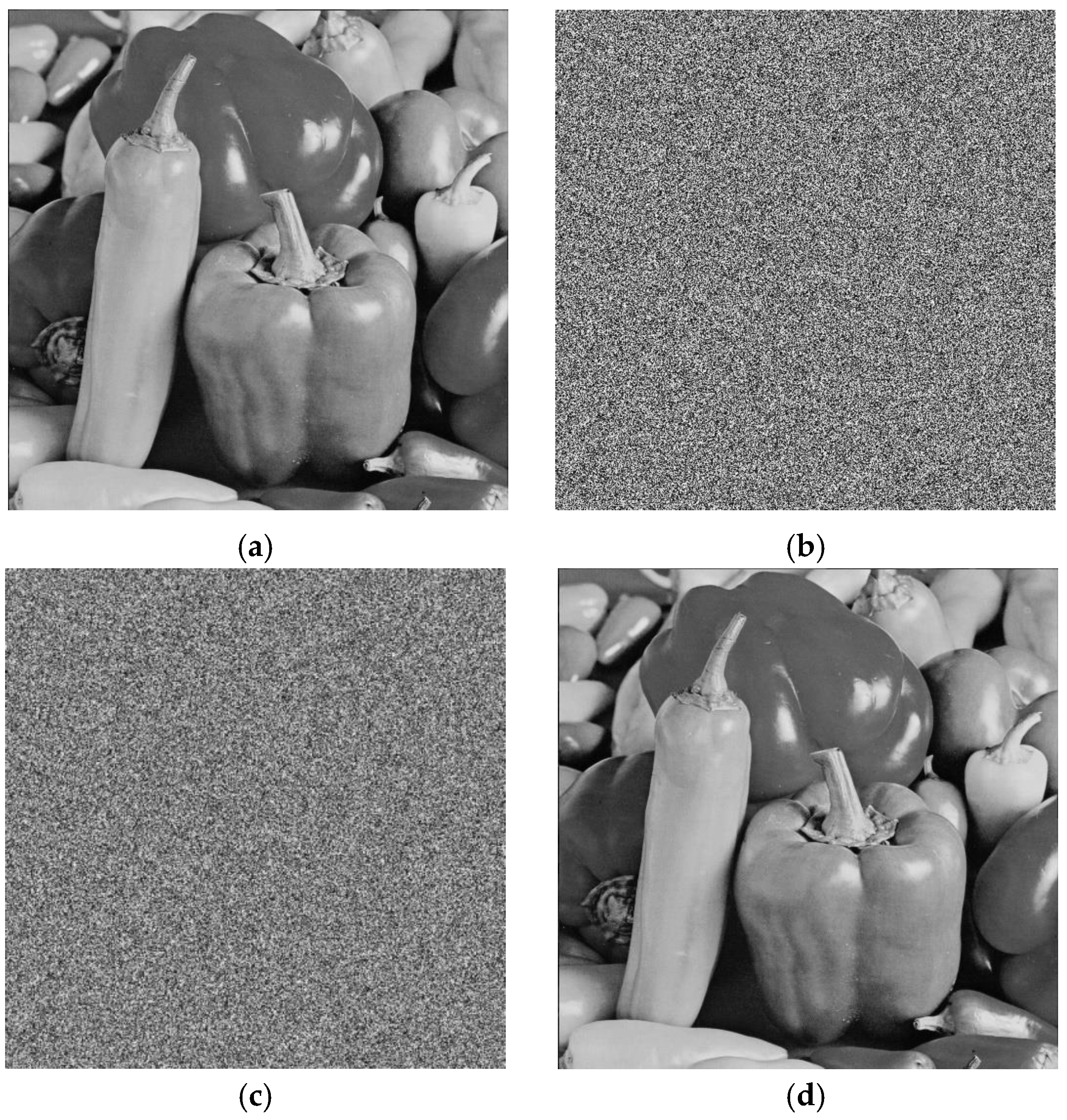
The example in Figure 5 presents the results of testing the ‘Pepper’ image, observing the changes in the image after different stages of processing. Through visual observation, it can be noted that there is no visual similarity between the original image (Figure 5a), the encrypted image (Figure 5b), and the stego image (Figure 5c). It means that from a visual quality perspective, our proposed scheme is secure and will not attack malicious attention and no information related to the original image or hidden secret data will be leaked.

3.2. Image Pixel Correlation

The pixel correlation of an image refers to the similarity or correlation between different pixels in the image. By analyzing the brightness differences or common variations between each pixel and its surrounding pixels, features such as texture, structure, and patterns can be revealed in the image. This kind of correlation analysis is crucial for many tasks in the field of image processing, such as image recognition, segmentation, enhancement, and compression, aiding in understanding and extracting information from the image, thus enabling various applications. In the security evaluation of image encryption schemes, the pixel correlation coefficient is a critically important indicator. It reflects the correlation between neighboring pixels in the image. Specifically, this refers to the relationship between the values of neighboring pixels in the image. We can evaluate the effectiveness of the encryption scheme by comparing the correlation between neighboring pixels in the original image and the encrypted image by using Equations (13)–(15).

$$E\left(x\right)={\displaystyle \frac{1}{W\times H}}\sum _{i=1}^{W\times H}{x}_i,D\left(x\right)={\displaystyle \frac{1}{W\times H}}\sum _{i=1}^{W\times H}{\left(x_i-E\left(x_i\right)\right)}^2.$$

(13)

$$cov\left(x,y\right)={\displaystyle \frac{1}{W\times H}}\sum _{i=1}^{W\times H}\left(x_i-E\left(x_i\right)\right)\left(y_i-E\left(y_i\right)\right).$$

(14)

$$p_{xy}={\displaystyle \frac{cov\left(x,y\right)}{\sqrt{D\left(X\right)D\left(Y\right)}}} .$$

(15)

Here, x and y are the pixel values of neighboring pixels in an image, and W and H is the width and height of the original image or encrypted image. It is noted that Equation (13) defines the mean E(x) and variance D(x) of pixel values in an image, where E(x) is the average value of the image’s pixel values, where W × H is the total number of pixels, and x_i represents the value of the i-th pixel. This mean value represents the overall brightness or grayscale level of the image. D(x) describes the distribution of pixel values, i.e., the degree to which pixel values deviate from the mean. A larger variance indicates that the pixel values are more dispersed, which corresponds to higher contrast in the image. Equation (14) defines the covariance cov(x, y) between two variables x and y, where x and y represent the values of adjacent pixels x and y. The greater the correlation between x and y, the larger the value of the covariance. In image pixel correlation analysis, covariance is used to measure the correlation between adjacent pixels. A larger covariance indicates a higher correlation between adjacent pixel values, while a covariance close to 0 indicates a lower correlation. Equation (15) defines the correlation coefficient p_xy between pixels, which represents the correlation between adjacent pixels by dividing the covariance by the product of the standard deviations. The range of the correlation coefficient p_xy is between −1 and 1. If p_xy approaches 1, it indicates a high positive correlation between the two pixels, meaning that adjacent pixel values in the original image tend to change in a similar manner. If p_xy approaches 0, it indicates that the two pixels are almost uncorrelated, which usually occurs in encrypted images because encryption disrupts the correlation between adjacent pixels, making the image appear more random. If p_xy approaches −1, it indicates a highly negative correlation, though this situation is rare in images.

By comparing the correlation of adjacent pixels in the image before and after encryption, the effectiveness of the encryption scheme can be analyzed. In the original image, adjacent pixels exhibit significant linear correlation, while after encryption, the randomization of pixel values reduces the correlation between adjacent pixels. Therefore, the encrypted image should show a lower correlation coefficient p_xy, which helps validate the effectiveness of the encryption scheme. Here, we select the horizontal, vertical, diagonal, and anti-diagonal directions as examples and demonstrate them in Figure 6 and Figure 7. By observing the distribution of neighboring pixels in the original and encrypted images, we can see significant differences. In the original image, neighboring pixels exhibit a clear linear correlation, as illustrated in Figure 6. In contrast, as shown in Figure 7, the distribution of neighboring pixels in the encrypted image is relatively uniform, indicating a lower correlation among them within the coordinate system. It is concluded that the encryption function works well in our proposed scheme.

The results presented in Figure 6 indicate that the neighboring pixels in the four directions of the original image are linearly correlated, reflecting the characteristic that adjacent pixels show a strong linear correlation. In contrast, the neighboring pixels in the four directions of the encrypted image, shown in Figure 7, are distributed more uniformly across the coordinate system. The findings in Figure 6 and Figure 7 confirm that the image encryption operations outlined in Section 2.1 are effective.

3.3. Image Histogram Analysis

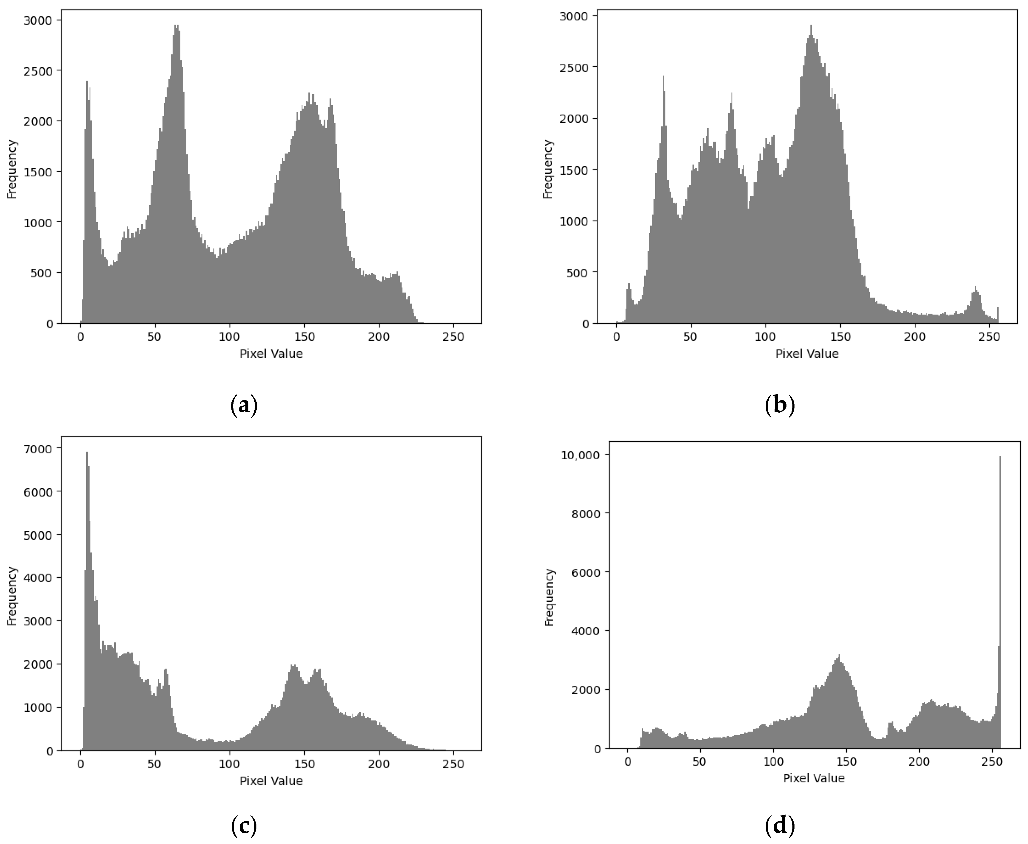
Image histogram analysis is a classic method of statistically analyzing and visualizing the pixel values of an image. It presents the image’s brightness, contrast, and color distribution in a histogram by counting the frequency of occurrence of each pixel value. By observing the shape and features of the histogram, we can conduct a preliminary analysis of the characteristics of the image, such as whether the brightness distribution is uniform and whether the contrast is sufficient. It shows the distribution of pixel values of each pixel in the range [0, 255] in the image. The histogram of the original image may exhibit a certain regularity, making the image more susceptible to statistical analysis attacks and thereby jeopardizing the security of the entire encryption scheme. Therefore, to enhance the security of the encryption scheme, a method must be sought to balance the histogram of the encrypted image.

When evaluating the image encryption scheme, we observed the histograms of the original images ‘Pepper’, ‘Deer’, ‘Dance’, and ‘City’, as well as their corresponding encrypted images, as shown in Figure 8 and Figure 9. We found that the histogram of the encrypted image shows a more uniform distribution of grayscale pixel values in the range [0, 255], with no discernible patterns. This means that the information of the original image cannot be recovered from the histogram of the encrypted image. Therefore, this encryption scheme demonstrates strong resistance to histogram analysis attacks. Through such observation and analysis, we can be confident that this encryption scheme performs well in protecting image security. By balancing the histogram of the encrypted image, we effectively increase the difficulty for attackers in performing statistical analysis on the encrypted image, thereby enhancing the overall security level of the encryption scheme.

3.4. Feature Comparison

In addition to validating the security performance of our proposed method, we also conducted experiments comparing it with other similar schemes [12,13,14,15,16] in the field of image embedding, to delve into the strengths and weaknesses of each approach. We not only compared the performance of the proposed method with other schemes in terms of PSNR and the embedding rate but also conducted difference comparisons based on [12]. These metrics provide a more comprehensive assessment to determine the advantages of our method. To comprehensively evaluate the performance of our proposed method, comparative experiments were conducted with five similar methods. Fifty images were randomly selected from the Bossbase image database, and the experimental results are shown in

Table 1. Comparison among five existing schemes and our proposed scheme.

	Chen et al. [12]	Hassan et al. [13]	Mandal et al. [14]	Bai et al. [15]	Zhong et al. [16]	Proposed Method
BPP	1.0349	1.1880	2.0129	1.4883	1.4553	2.1111
PSNR	35.8347	34.1092	33.6419	30.7286	39.2284	35.2410
BPP Difference	0	0.1531	0.9780	0.4534	0.4204	1.0762
PSNR Difference	0	−1.7255	−2.1928	−5.1061	3.3937	0.5937

.

By comparing the embedding rates, which refer to the amount of data embedded per pixel, we found that our bpp is still slightly higher than that of Mandal et al. [14], maintaining approximately 1.60 more dB compared to their results. Moreover, our proposed method places more emphasis on data concealment and security. This is because the experimental data all use unencrypted PSNR, and our method does not involve LSB or the most significant bit (MSB) replacement. Based on the data results, our method shows a significantly higher PSNR than other similar methods. To ensure data security, the proposed method replaces the pixel values after embedding data, deliberately reducing the quality of PSNR. Decreasing PSNR means the ability to blur or hide details in the image, which is a useful technique in privacy or copyright protection. For instance, in scenarios where identity needs protection or sensitive information needs to be handled, blurring the image can help reduce identifiable information. While maintaining data fidelity and preventing data overflow, our method still provides a higher embedding rate, achieving the effects of reversible data extraction and image recovery. These are significant advantages of our method. Therefore, our research not only focuses on data concealment and protection but also considers how to achieve a high embedding rate through these means, comprehensively evaluating the performance of our proposed method. This comprehensive analysis gives our method a significant competitive advantage in the field of image processing.

3.5. True Positive Rate

The True Positive Rate (TPR) is a measure used in statistical analysis, particularly in binary classification. TPR measures the proportion of actual positive cases that are correctly identified by a model. A high TPR indicates how well the model is able to detect positive cases. TPR is defined as

$$\mathrm{TPR}= {\displaystyle \frac{TP}{TP+FN}}$$

(16)

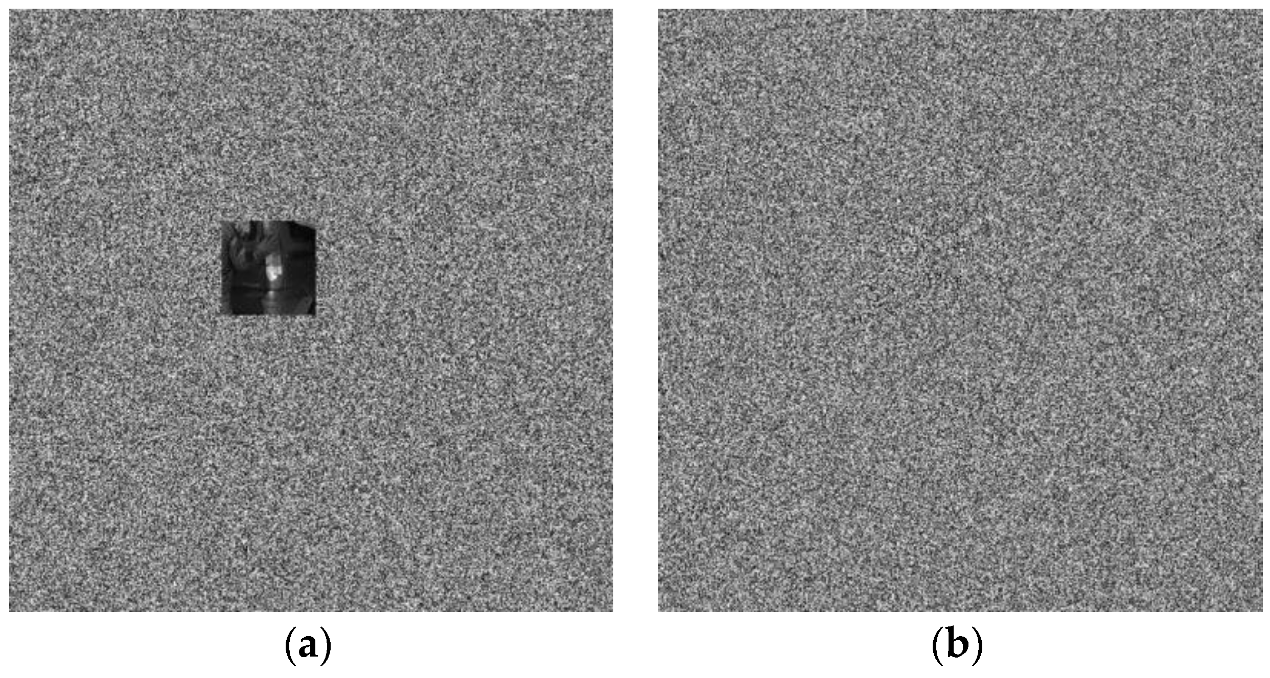
where TP is true positive and FN is false negative. TP means the cases where the model correctly predicts a positive outcome, and FN denotes the cases where the model fails to predict a positive outcome that actually exists. As shown in Figure 10, two types of collage attacks are conducted to test the performance of tamper detection. The first attack tampers an image by copying image blocks from a plaintext image and inserting them to arbitrary positions in the encrypted stego image. The second attack forges an image by copying encrypted blocks from an encrypted image and inserting them into arbitrary positions in the encrypted stego image.

Figure 11 shows the tamper results of “Pepper”. Some blocks are replaced by the blocks copied from the other plaintext image and an encrypted image. The tamper detection results delivered by the proposed scheme are listed in

Table 2. The tamper detection results under different attacks.

	Peppers	City	Dance	Deer
TPR of the first attack	86.50%	88.81%	86.25%	88.69%
TPR of the second attack	88.25%	86.25%	86.56%	87.19%

. We use the 3-bit authentication data to detect any changes or alterations made to the encrypted stego image. Obviously, there is a 1/8 probability of a collision occurring, leading to incorrect detection results. Therefore, we propose a hierarchical tamper detection strategy to further refine the tamper detection results.

Table 3. The hierarchical tamper detection results under different attacks.

	Peppers	City	Dance	Deer
TPR of the first attack	99.99%	100.00%	99.99%	99.99%
TPR of the second attack	99.92%	99.93%	99.90%	99.90%

lists the hierarchical tamper detection results for two types of attacks. We can see that the hierarchical strategy offers a higher TPR, which represents most actual positive cases are correctly identified by our scheme. The results show that our scheme can authenticate or verify an image as true while ensuring that the image content remains protected through encryption.

4. Conclusions

In this paper, we propose a reversible and authenticable data-hiding scheme for encrypted images with a combination of interpolation technology and substitution, aimed at enhancing the security of encrypted images and the capacity for data hiding. Our scheme provides higher hiding capacity while maintaining the confidentiality of the secret data and cover image. With our encryption and scrambling operations, our proposed scheme can ensure that there is no information on the cover image will be leaked without the encryption key. Moreover, the embedded authentication data helps to verify the authenticity of the image and provides the ability to localize the tampering. Consider that there are many representative encryption algorithms, proven to offer high security, which can serve as alternatives to our proposed image encryption approach. In the future, our next steps will focus on improving the authentication function and potentially providing a recovery function.