Advanced Scanning Technology for Volume Change Measurement of Residual Soil

Abstract

Weathering processes of rocks lead to the formation of residual soil layers, which are typically characterized by a deep groundwater table and a thick unsaturated zone. Hence, the calculation of a slope’s safety factor under the influences of climatic circumstances is a function of unsaturated characteristics, such as the soil–water characteristic curve (SWCC). To determine the SWCC, the volume of the soil specimen must be determined in order to compute the void ratio and degree of saturation. The drying processes of the soil specimen led to uneven soil volume change during laboratory SWCC testing, demanding the development of a soil shrinkage curve. Several methods for measuring soil volume change have been developed over the years. However, there are significant limitations, and it is rarely used due to the difficulty linked to accurately measuring the soil volume during drying processes. In this study, a revised scanning approach is developed to evaluate residual soil volume change utilizing 3D scanning technology. The proposed method is applied in a case study on residual soil from the Old Alluvium in Singapore. The laboratory data and analysis results suggested that 3D scanning technology should be required to provide a correct estimation of the air-entry value of soil.

1. Introduction

Singapore has a tropical climate accompanied by heavy rainfall, high temperature, and high humidity during the year due to its location close to the equator [1]. Depending on the mineralogy of the parent rock, the degree of the weathering, the amount of rainfall, and the temperature, such environments may produce distinct engineering and index properties [2]. Therefore, residual soil is formed in thick layers and typically placed in four major geological formations: Bukit Timah Granite, Kallang Formation, sedimentary Jurong Formation, and Old Alluvium Formation in Singapore [3]. Such soils shrink both horizontally and vertically as a result of moisture evaporation. Residual soils, a kind of problematic soils, are prone to shrink by a significant amount in periods of intense drying following heavy wet seasons [4].

The porous soil structure that was brought about by the leaching of specific types of soil minerals, during which water and air replaced the soluble minerals, along with the geochemical transformations associated with weathering, such as the formation of new minerals like clay, leading to a very high void ratio, are affected by a deep groundwater table on many residual soil slopes [5]. The zone between the groundwater table and the soil surface is called an unsaturated zone, which is very sensitive to variations in climatic conditions [3]. One of the key properties of unsaturated soil is the soil–water characteristic curve (SWCC), which essentially illustrates the relationship between soil suction and water content [6]. SWCC can be presented in the form of gravimetric water content, volumetric water content, and degree of saturation. These three forms of SWCC are differentiated based on the dependency on soil volume change [7]. Since the shrink–swell phenomenon in the soil only affects a set depth known as the active zone, measuring volumetric water content and degree of saturation requires a shrinkage curve [4]. As water content in soil decreases from full saturation to a dry state, the shrinkage curve describes the relationship between void ratio and water content [8,9]. This relationship is critical because as unsaturated soils lose water, their volume reduces due to the shrinkage of the soil matrix. Neglecting this volume change can lead to inaccuracies in measuring the volumetric water content and degree of saturation [10].

Many researchers concluded that the SWCC is associated with the degree of saturation, which is very important in the determination of air-entry value and the permeability function of soil [11]. In the geotechnical design, with respect to the effect of rainfall, the SWCC corresponding to volumetric water content is one of the main parameters in running transient seepage finite element analyses [12,13,14]. In numerical analyses, there is a lot of demand for SWCCs with respect to volumetric water content and degree of saturation, indicating the significance of the shrinkage curve in unsaturated soil analysis [15,16,17]. Hence, there is a need to have an appropriate measurement of soil volume change for the development of a shrinkage curve.

Past research has faced plenty of challenges in obtaining accurate measurements of volume change during SWCC tests [18,19]. The challenges in determining the shrinkage curve were mostly due to the presence of cracks and non-homogeneity in the reduction in soil dimensions during the drying process. Other challenges were linked with the methodologies and technologies utilized to measure soil volume change. Manual measurement using Vernier calipers is the most common method for determining the shrinkage curve. It is easy, cheap, and non-destructive; however, it is limited to homogeneous specimens [20,21,22]. This method does not produce high-quality results for an irregular shape of a specimen.

The volume displacement method could produce a better measurement of soil volume. This method requires the specimen to be wrapped with wax or equivalent materials prior to submergence into water [23,24]. The soil volume measurement is determined from the amount of liquid displaced by the specimen’s volume following Archimedes’ law. This method can provide a reasonable measurement of the irregular shape of the specimen. However, this technology is destructive when the specimen has large pores [25]. The wax particle may fill in the voids between solid particles, and it may weaken the bonding between each grain. In addition, the wax may not be in proper contact with the specimen, leading to an inaccurate volume measurement.

The emergence of digital imaging technology contributes to the popular technique of volume change measurement of the specimen using a digital camera. Li et al. [26] proposed imaging technology to measure the volumetric strain of expansive soil using a digital camera. During the drying process, they photographed the top, sides, and bottom of the specimens. The restriction of this approach is the formation of cracks. It is difficult to obtain an accurate measurement of the depth of a crack using many photo combinations. Sander and Gerke [27] and Stewart et al. [28] developed 3D scanning technology called “Clodometer”. This technique required a reference object with known volume as a reference to measure specimen volume for each corresponding time. As a result, cumulative errors at the end of specimen volume measurement are quite large, resulting in an inaccurate volume change.

Some researchers utilized the image correlation method, particle image velocity (PIV), to obtain the volume change in specimens based on the time-sequence displacement field [29,30,31]. This technique combines a 2D planar image from different directions. Therefore, PIV requires proper calibration of the digital camera prior to the test to avoid distortion due to the effect of the camera lens. The error can be quite significant if the calibration is not performed correctly, even though the image is taken from the same plane. This method is also not applicable for soil with the occurrence of cracks during the drying process. Jain et al. [32] incorporated laser into photogrammetry to improve the accuracy of image scanning using the triangulation method for deformation monitoring. They observed that the error was only 1% during the image processing. The limitation of this technique is the assumption of specimen uniformity. In practice, obtaining a consistent soil surface is difficult, especially if the soil is classified as worn rock. Li and Zhang [33] proposed a novel method for improving the quality of photogrammetric post-processing images. The volume measurement error was roughly 0.4%. However, prior to testing, this procedure necessitates highly accurate calibration of the digital camera. Furthermore, the post-processing image requires transformation from 2D to 3D images, which may result in problems if not conducted correctly.

Understanding the soil shrinkage curve is essential for geotechnical engineering implementation, as it directly influences the assessment of soil behavior under varying moisture conditions. Knowledge of this curve enables engineers to predict changes in soil volume, which can lead to issues such as settlement, heave, and instability in structures [34,35,36]. Accurate modeling of shrinkage behavior is crucial for designing foundations, slopes, and earth-retaining structures, as it informs the selection of appropriate materials and construction methods [11]. Furthermore, understanding the shrinkage characteristics of soil aids in evaluating the long-term performance and durability of geotechnical systems, ensuring that infrastructure can withstand environmental changes [37]. Incorporating the soil shrinkage curve into geotechnical assessments is therefore vital for enhancing project safety and effectiveness.

The limitations of past methods for measurement of soil volume change are associated with the high-accuracy equipment which does not need complex and tedious calibration. In addition, there are only limited studies with respect to the advanced measurement of soil volume change for residual soil. Therefore, the advanced methodologies for measuring soil volume change utilizing modern 3D scanning technology are proposed in this work. The change in soil volume caused by SWCC measurement is modeled by combining a shrinkage curve with the measured SWCC in terms of gravimetric water content. Under unsaturated conditions, the coefficient of permeability, which is a function of void ratio and water content, is estimated from the SWCC. A commonly used technique is a statistical method proposed by Childs and Collis-George [38], which uses parameters that account for soil texture and pore structure along with the SWCC to provide an alternative to direct measurement of permeability. However, the shape of the permeability function is affected by the shape of the SWCC. Hence, the unsaturated permeability estimated from SWCC with soil volume change will be different from that without soil volume change. The research entails the creation of methods for accurate assessment of soil volume utilizing the proposed 3D scan technology, laboratory experiments involving the SWCC test, shrinkage test, 3D scan, and determination of the air-entry value of a residual soil from Singapore.

2. Residual Soil and Geological Formation

Residual soils are developed because in situ physical, chemical, and biological weathering affect parent rock formation [39]. Physical weathering occurs when the earth or surrounding environment moves, leading to the rock formation breaking. Chemical weathering occurs when chemicals dissolved in rainwater react with the minerals found in rocks. Furthermore, the underground rock formation is influenced by the strains and tensions generated by the plant roots that grow on it. Thus, biological weathering can lead rock formations to break [19,40]. Weathering processes cause residual soil layers to accumulate on the parent rock formation over time. This is especially true in tropical climate countries with year-round high temperatures, high humidity, and excessive rains [3]. As shown in Figure 1, Singapore has four major geological formations with thick residual soil layers: Bukit Timah Granite, Kallang Formation, sedimentary Jurong Formation, and Old Alluvium Formation. Bukit Timah Granite is mostly found in the country’s northern and central regions. The majority of the rocks in Bukit Timah Granite are granite and granodiorite [7]. Reddish to yellowish brown silty soils occur in the top layers of Bukit Timah Granite.

Old Alluvium Formations is the oldest among the drift deposits. Old Alluvium is an extension of southern Johore deposits, and they form a continued plate in east Singapore [41]. The area of the Old Alluvium is around 12 km² and is located in the northwestern part of Singapore, as displayed in Figure 1. However, the formation is situated mostly in the island’s eastern part and is formed as a near-successive plate at the top and bottom of younger deposits [41]. The soil of the Old Alluvium Formation is mainly reddish muddy dense sand with clay and silt [40]. The soil’s density varies from loose sand closer to the surface to stiff clay at larger depths.

Residual soils can be divided into six categories (Grade I–VI) depending on the weathering extent of geological formation [42]. Grade I is the fresh rock (parent rock formation), whereas Grade VI is entirely weathered soil (residual soil). The grade rises with the increasing degree of weathering and atmospheric exposure. Higher-grading residual soils mainly have an increased ratio of fine particles as clay and decreased density due to continuous weathering processes [3]. Consequently, the shear strength of higher-grade residual soils has been reduced compared to that of their parent rock. Due to their larger pores, lower-grade residual soils have a higher potential to leach, whereas higher-grade residual soils have a higher capacity to hold water [43]. Residual soils in Jurong Formation tend to be finer and less uniform than Old Alluvium and Bukit Timah Granite residual soils [44,45]. When residual soils are developed on a slope, it may lead to slope instability and failure, specifically when water enters the soil. Therefore, it is essential to comprehend unsaturated soil behavior and to define the soil–water characteristic curve, including the required volume change measurement.

With the increasing depth, the effective cohesion (c′) value decreases because of the decrease of fine particles. Bukit Timah Granite residual soils have lower effective cohesion than Jurong Formation and Old Alluvium residual soils. The proportion of sand, on the other hand, increases with increasing depth, which corresponds to a rising effective friction angle (ϕ′) [3]. The saturated permeability of residual soils of Bukit Timah Granite ranges between 10⁻¹⁰ and 10⁻⁵ m/s [46]. This was later confirmed by Zhang et al. [47] with an extensive empirical study of Bukit Timah Granite, which indicates a great extent of saturated permeability for residual soils of Bukit Timah Granite.

3. Mathematical Equations

In the SWCC tests, the change in the mass of a soil specimen is usually recorded, but the total volume change in the specimen is not measured. Therefore, the gravimetric water content versus soil suction of a soil specimen is plotted in the SWCC. However, according to Fredlund et al. [11] and Zhai et al. [48], the volume change in a soil specimen may be significant and important to the data interpretation of the SWCC. Hence, the shrinkage curve is established by measuring the volume change in a soil specimen as it progressively loses moisture during the drying process. A relationship between the void ratio and gravimetric water content of a soil specimen is then formed and used in conjunction with the SWCC. A shrinkage equation that fits a wide variety of soils was proposed by Fredlund et al. [11], as can be seen in Equation (1):

$$e (w)=a_{sh} {\left[{\displaystyle \frac{({w)}^{C_{sh}}}{{{(b}_{sh})}^{C_{sh}}}}+1\right] }^{{\displaystyle \frac{1}{C_{sh}}}}$$

(1)

where $e \left(w\right)$ is the void ratio of the soil specimen; $a_{sh}$ is the minimum void ratio of the soil specimen; $b_{sh}$ is the slope of the tangency; $C_{sh}$ is the curvature of the shrinkage curve; and $w$ is the gravimetric water content of the soil specimen.

The SWCCs, in terms of the volumetric water content and degree of saturation of a soil specimen versus soil suction, are plotted to determine the correct air-entry value and compute the unsaturated soil property functions of the soil specimen [11]. Fredlund and Xing [49] developed a general SWCC model (Equation (2)) to best fit the unimodal SWCC based on the pore-size distribution of soil, and it has been observed to fit well with experimental data for a suction range from 0 to 106 kPa. A later study conducted by Leong and Rahardjo [50] also concluded that Fredlund and Xing’s [49] equation better fits the SWCC among all the various equations.

$${\theta }_w=\left[1-{\displaystyle \frac{\mathit{ln} \left(1+\frac{\psi }{c_r}\right) }{\mathit{ln} \left(1+\frac{{10}^6}{c_r}\right)}}\right]{\displaystyle \frac{{\theta }_s}{{\left\{ \mathit{ln} \left[e+{\left(\frac{\psi }{a}\right)}^n\right] \right\}}^m}}$$

(2)

where ${\theta }_s$ is the saturated volumetric water content; $\psi$ is the matric suction (kPa); $C_r$ is the matric suction corresponding to the residual water content (kPa); $a$ is the fitting parameter of SWCC and is closely related to the air-entry value of the soil; $n$ is the fitting parameter of SWCC and controls the slope at the inflection point of SWCC; and $m$ is the fitting parameter of SWCC and is closely related to the residual water content.

Satyanaga et al. [51] adopted (Equation (3)) as the best-fitting SWCC with a dual sub-curve (bimodal SWCC). This equation needs the correction factor $\left(C_{\left(\psi \right)}\right)$ to guarantee that the water content is negligible at 1 GPa of soil suction.

$${\theta }_w=C_{\left(\psi \right)}\left[\begin{array}{c}{\theta }_r+\left({\theta }_{s1}-{\theta }_{s2}\right)\left(1-erfc{\displaystyle \frac{\mathit{ln} \left(\frac{{\psi }_{a1}-\psi }{{\psi }_{a1}-{\psi }_{m1}}\right) }{s_1}}\right)+\left({\theta }_{s2}-{\theta }_r\right)\\ \left(1-erfc{\displaystyle \frac{\mathit{ln} \left(\frac{{\psi }_{a2}-\psi }{{\psi }_{a2}-{\psi }_{m2}}\right) }{s_2}}\right)\end{array}\right]$$

(3)

where ${\theta }_w$ is volumetric water content at any suction; ${\theta }_s$ is saturated volumetric water content; $\psi$ is soil suction of the soil (kPa); $a$ is soil parameter that is primarily determined by the soil’s air-entry value (AEV) (kPa); $n$ is a function of the rate of soil water extraction when the AEV has been reached; $m$ is a function of the residual water content; ${\psi }_m$ is soil suction at the inflection point (kPa); ${\psi }_a$ is the air-entry value of soil (kPa); and $s$ is the geometric standard deviation of SWCC.

4. Proposed Soil Volume Change Measurement Procedures

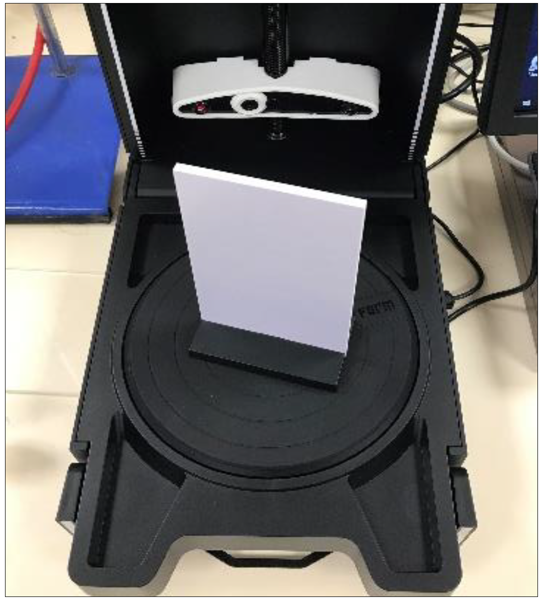
Due to the irregularities of a soil specimen during drying, a three-dimensional (3D) scanner was used to capture a precise and accurate 360$°$ view of the soil specimen. A Matter and Form Scanner with the optics of a high-definition sensor and two Class 1 eye-safe lasers with a scanning accuracy of within ±0.1 mm was utilized in the 3D scanning test. The 3D scanner requires MFStudio software v2, which can be downloaded from https://www.matterandform.net/pages/v2 (accessed on 21 November 2024). Prior to the commencement of the scanning process, the 3D scanner needs to be calibrated, and a calibrating card should be placed on the 3D scanner for proper calibration, as shown in Figure 2. When the 3D scanner is moved or the lighting situation changes substantially, it is advised that it be calibrated.

The MeshLab and Meshmixer software are available for download at http://www.meshlab.net/#download (accessed on 19 November 2024) and http://www.meshmixer.com/download.html (accessed on 19 November 2024), respectively. MeshLab software is required for meshing and trimming cloud points and measuring the volume of the solid soil specimen. Meanwhile, the Meshmixer software is necessary to convert the cloud point into a solid soil specimen. The initial stage in 3D scanning soil specimens in a shrinkage test was to place a soil specimen covered in plastic film on the scanner turntable. Prior to scanning, the following criteria should be met.

(a)

The bottom surface of the soil specimen is flat, as the surface will not be captured in scanning and is assumed to be flat when editing the cloud point.

(b)

The plastic film has no fines or stains, especially around the circumference of the soil specimen.

The option ‘Laser 1’ in the MFstudio software should be selected for greater accuracy of scanning. To achieve great accuracy in the scanning process, the following settings should be used:

(a)

For a good set of laser lines, the geometry should be set to 60% or adjusted according to the lighting changes in the environment.

(b)

Texture settings should be set to 60% for optimal color capture exposure, and texture capture should be turned off. Otherwise, the settings should be adjusted to match the soil specimen’s color and texture.

(c)

If the height of the soil specimen is different, adjust the vertical scan path accordingly.

(d)

For scanning a soil specimen with a height of 30 mm, the vertical scan path should be set to two bars. If the height of the soil specimen is different, the vertical scan path should be modified accordingly.

(e)

The horizontal scan path should be increased to 100% to scan the entire soil specimen in 360°.

After adjusting to the required settings, the quick scan that generally takes about 4 min should be carried out with the above settings. When the scanning is completed, any unwanted points of the point cloud may be cleaned using the editing tools. Editing the point cloud with a brush cleaning tool is advised for accuracy. Figure 3 shows the point cloud of a soil specimen after editing in MFstudio. The file should be exported using ‘Export’ under the file menu and saved as XYZ files. Then, the ‘Import Mesh’ under the file menu should be chosen by opening the previous XYZ file in the MeshLab software.

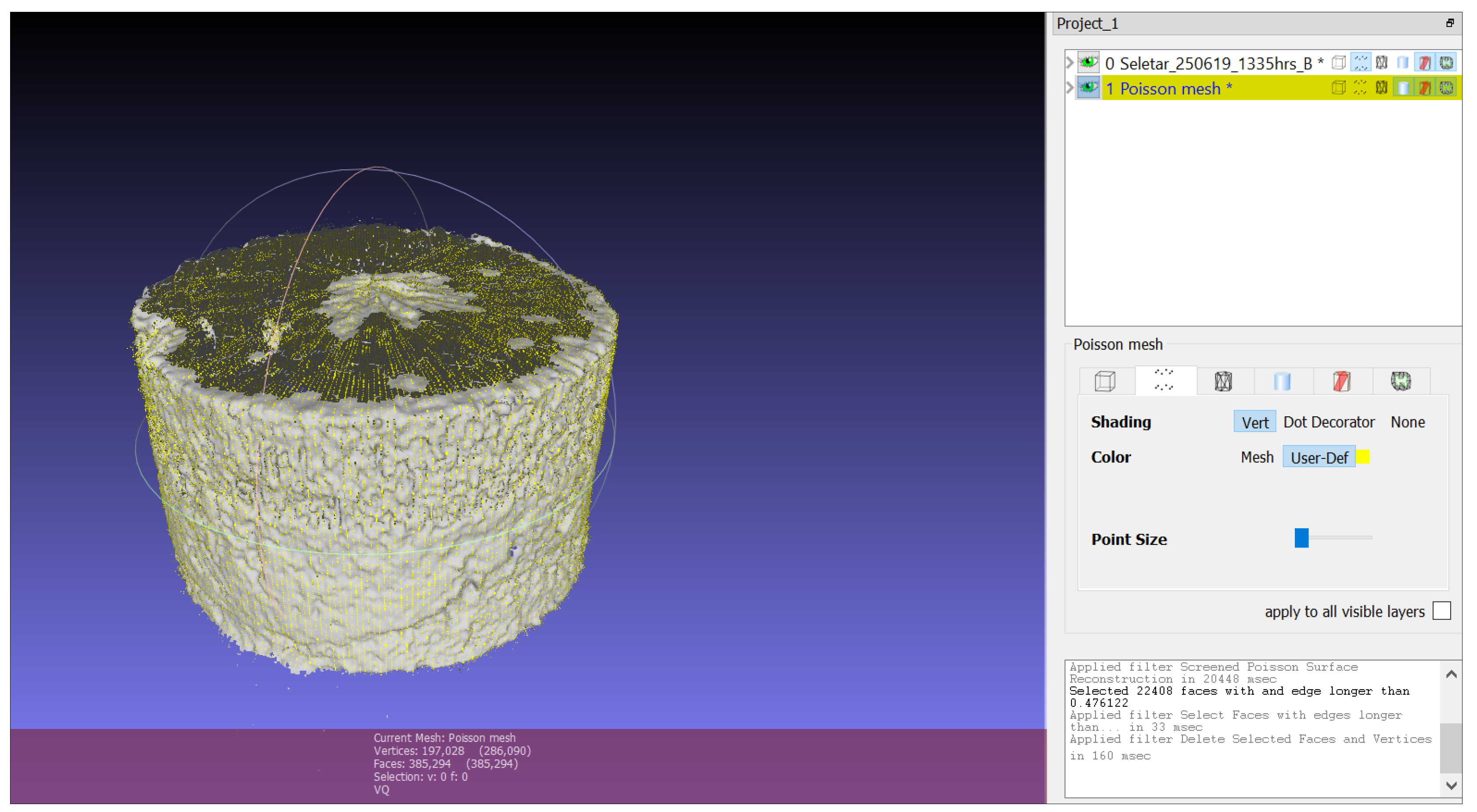
The point cloud of a soil specimen will appear, as shown in Figure 4. Under the filter’s ‘Normals, Curvatures and Orientation’ menu, the ‘Compute normals for sets’ should be selected, and an appeared pop-up box should be closed by clicking ‘Apply’ with the default setting. In addition, ‘Screened Poisson Surface Reconstruction’ should be picked from the filter’s ‘Remeshing, Simplification, and Reconstruction’ menu, and a pop-up box will emerge. After creating an exterior mesh, the pop-up should be closed by clicking ‘Apply’. The newly constructed Poisson mesh layer should be chosen in the right-hand panel. Then, ‘Select Faces with edges longer than’ should be picked from the ‘Selection’ menu of the filter, and a small pop-up window will appear. The pop-up box should be closed by clicking ‘Apply’ with the default edge threshold setting. The edges beyond the point cloud’s threshold must be picked and highlighted in red. Subsequently, under the filter’s menu of ‘Selection’, the ‘Delete Selected Faces’ must be chosen. The protruding edges will be trimmed away, as shown in Figure 5.

A file name should be specified (e.g., LOCATION OF SOIL DDMMYY HH: MM C) and saved as an STL file by choosing ‘Export Mesh as’ under the file menu. After the file is saved successfully, the Meshmixer software may be opened, and the file should be imported. The previous STL file should be located and opened. The mesh of a soil specimen will appear in Meshmixer, where after a solid soil specimen is formed, the ‘Make Solid’ under the edit tab should be selected, as shown in Figure 6.

Subsequently, ‘Inspector’ should be chosen under the analysis tab. ‘Auto Repair All’ and ‘Done’ are available options. This function examines the solid soil specimen for flaw holes and seals them, making it watertight. By selecting ‘Export’ under the file menu, the file should be saved in STL ASCII format (e.g., LOCATION OF SOIL_DDMMYY_HH: MM_D). Then, the previous STL ASCII file may be imported into the MeshLab software. Afterwards, the volume of the solid soil specimen may be obtained by selecting ‘Computer Geometric Measures’ under the filter’s menu of ‘Quality, Measure and Computations’. If an error indicates that the mesh is not watertight, this extra step is required. The ‘Close Holes’ filter should be selected and applied from the ‘Remeshing, Simplification, and Reconstruction’ menu. This technique should then be repeated to determine the volume of the solid soil specimen. Meshmixer can also be used to measure the volume of solid soil specimens. The ‘Stability’ button can be picked under the analysis tab, and a side box with volume will appear, as shown in Figure 7. Finally, under the same tab, ‘Orientation’ should be selected to rotate the solid soil specimen into an upright position.

5. Testing on Residual Soil

A Gel-Push (GP) method of data collection adopted from Taylor et al. [52] was applied to gather the undisturbed soil specimen across distinct sites, such as Tampines (with a 3–4 m depth) and Seletar Hill (3–4 m depth). The GP method is an innovative technique for collecting soil samples that involves using a specialized probe to insert a viscous gel into the soil at a desired depth. This gel encapsulates soil particles, minimizing disturbance and preserving the in situ properties of the sample. Once the probe is withdrawn, the gel, along with the collected soil, is extracted, allowing for easier transportation and analysis while maintaining the integrity of the sample. Figure 1 illustrates the landmarks of the soil specimens mentioned along Singapore’s topographic map. Onward, with a test hole physically excavated toward a level ranging from 1.5 m, the earth has been bailed about a level between 1.5 and 3.0 m. The GP tester was again used throughout soil exploration for the collection of undisturbed samples of soil with high-quality. The GP tester also employs a polymer solution with a high concentration to lessen the resistance within the soil specimen and collecting pipe. Throughout the research lab, individual samples taken were once again manually compressed one by one from tester pipes. Following that, earth samples were cut to the necessary length and width for numerous scientific tests.

After extrusion, the samples were subjected to index property tests to determine various index soil qualities. The tests were conducted according to the standards outlined in

Table 1. Index properties testing standards.

Index Properties Test	Testing Standards
Specific gravity	ASTM D854-14 [54]
Grain-size distribution	ASTM D422-63 [55]
Atterberg limits	ASTM D4318-17e1 [56]
Soil Classification (Unified Soil Classification System)	ASTM D2487-17 [57]

. The ASTM D6836-16 was used to perform laboratory tests to determine the drying SWCC [53]. The following equipment was used for measurements of SWCC in this study: a Tempe Cell and 1 bar ceramic disk, a Pressure Plate and 5 bar ceramic disk, and a WP4C Dewpoint Potentiometer. The soil sample was cylindrical in shape with a height of 5 cm and a diameter of 5 cm.

Prior to the SWCC test using Tempe cell, the one-bar ceramic disk was saturated in a desiccator with deaired distilled water. The soil specimen was then set into the Tempe cell. The specimen was saturated by applying de-aired distilled water from the top of the Tempe cell. The saturation process was ceased when the water content of the soil specimen reached its saturated value of at least 95%, which is the typical value adopted in practice for saturation of soil samples [53]. After the saturation stage, the weight of the saturated specimen and the Tempe cell was recorded. The air pressure system was connected from the top of the Tempe cell. Air pressure was then applied to the specified value to create respective matric suction in the soil specimen. Air would not flow through the porous ceramic disk when higher air pressure was introduced into the cell, as long as the air pressure did not exceed the air-entry value of the ceramic plate, and the ceramic plate was kept saturated. For this reason, the bottom of the Tempe cell was connected to a container filled with water to maintain the degree of saturation of the ceramic disk. Weighing the specimen at regular intervals was necessary to obtain sufficient data for the plot of the water volume change in the specimen at various matric suctions.

The pressure plate consists of a pressure chamber that contains a saturated five-bar ceramic disk. The pressure plate was connected to a burette for measurement of water volume change and maintenance of degree of saturation of the ceramic disk. There must be a good contact between the soil specimen and the ceramic disk to ensure the water flow between the specimen and the ceramic disk is continuous. As with the Tempe cell test, the specimen was weighed at regular intervals. When equilibrium was reached, a higher pore-air pressure was then applied.

The WP4C Dewpoint Potentiometer was utilized to measure the water potential of a soil specimen. The specimen is equilibrated with the headspace of a sealed chamber, containing a mirror. At equilibrium, the water potential of the air in the chamber and the water potential of the specimen become the same. The mirror temperature is controlled by a thermoelectric (Peltier) cooler. A photoelectric cell detects the exact point at which condensation occurs on the mirror. The device directs a beam of light onto the mirror reflecting into a photodetector, which senses the change in reflectance when condensation occurs on the mirror. A thermocouple, attached to the mirror, records the temperature at which condensation occurs. Values start to be displayed, and this indicates that initial measurements are being recorded. A green LED is flashed with a beeping sound when it reaches the final value. The final water potential and temperature of the specimen are displayed on the screen of the device. The device uses an internal fan that circulates the air within the specimen chamber to reduce the equilibrating time. The WP4C Dewpoint Potentiometer measures the total suction (sum of the osmotic and matric suctions) in the soil specimen. Soils bind water mainly through matric forces and therefore dominate the matric component, especially at low water content.

The shrinkage test was carried out on soil specimen with 5 cm diameter and 3 cm height. The soil specimen was exposed to air evaporation for a certain period of time. 10 sets of 3D scan tests on different soil specimens from the same soil type were conducted to ensure the reasonableness of shrinkage curve. Soil volume change measurement using 3D scanning involves capturing high-resolution data (following procedures explained in Section 4) was carried out to monitor changes in soil dimensions over time. The measurement of soil volume and water volume was conducted three times a day until the soil volume and water volume was considered constant. The measurement data of soil volume change was converted into void ratio, whereas the measurement data of water volume change was converted into gravimetric water content. The void ratio was plotted against gravimetric water content to generate the shrinkage curve. The discrete data of shrinkage curve was best fitted using Equation (1). The discrete data from SWCC test using Tempe cell, pressure plate, and WP4C were best fitted using Equation (2) (for unimodal SWCC) or Equation (3) (for bimodal SWCC). Then, the fitting parameters of Equation (1) were used to calculate the void ratio for every gravimetric water content in the SWCC plot generated using either Equation (2) or Equation (3). Finally, SWCC in terms of degree of saturation against soil suction can be plotted.

6. Results

The specific gravity, grain-size distribution, Atterberg limits, and soil classification are shown in

Table 2. Index properties.

Properties	Value
Bulk density, $\rho$ (Mg/m3)	2.15
Water content, $w$ (%)	16.3
Void ratio, $e$	0.42
Liquid limit, LL (%)	52
Plastic limit, PL (%)	24
Plasticity index, PI (%)	28
Specific gravity, $G_s$	2.65
Grain size distribution—gravel (%)	6
Grain size distribution—sand (%)	52
Grain size distribution—silt (%)	20
Grain size distribution—clay (%)	22
Unified Soil Classification System (USCS)	MH
Saturated coefficient of permeability, $k_s$ (m/s)	2.65 × 10−6

. It can be seen that the soil consists predominantly of fines, exhibits high plasticity, and can be classified as MH soil under the Unified Soil Classification System (USCS). Figure 8 depicts the w-SWCC data for the Tampines soil specimen. The $w$-SWCC discrete data are fitted using Equation (2) since it shows unimodal shape. The measurement data of soil and water volume change with time using the proposed 3D scan method are converted into void ratio against gravimetric water content, called shrinkage curve. Figure 9 shows the average data of shrinkage curve from 10 sets of 3D scans. The SWCC data, in terms of degree of saturation against suction ($S_r$-SWCC), are established using the shrinkage curve from 3D scanning measurements. Figure 10 depicts the $S_r$-SWCC for Tampines specimen with shrinkage curve from 3D scan measurement. The discrete data of the SWCC in Figure 10 are best fitted using Equation (3) since it shows a bimodal shape. Figure 11 shows the $S_r$-SWCC for the Tampines specimen after ignoring the shrinkage curve from the 3D scan data. The discrete data of SWCC in Figure 11 are best fitted using Equation (2) since it shows a unimodal curve. To prevent excessively large $m$, $n$, and ${\theta }_s$ values, these parameters are limited to a maximum of 6.

Table 3. SWCC parameters in saturation degree, using shrinkage curve from 3D scan.

SWCC Parameters		Value
Sub-curve 1	Air-entry value of sub-curve 1, ${\psi }_{a1}$ (kPa)	320
	Suction at inflection point of sub-curve 1, ${\psi }_{m1}$ (kPa)	1500
	Saturated degree of saturation of sub-curve 1, ${\theta }_{s1}$ (%)	100
	Standard deviation of sub-curve 1, $s_1$	2.5
Sub-curve 2	Air-entry value of sub-curve 2, ${\psi }_{a2}$ (kPa)	125,000
	Suction at inflection point of sub-curve 2, ${\psi }_{m2}$ (kPa)	200,000
	Degree of saturation of sub-curve 2, ${\theta }_{s2}$ (%)	40
	Standard deviation of sub-curve 2, $s_2$	1.0
Residual suction, ${\psi }_r$ (kPa)		4800

and

Table 4. SWCC parameters in saturation degree, discarding shrinkage curve from 3D scan.

Properties	Value
$a$	600
$n$	1.6
$m$	0.5
$C_r$	1500
Residual suction, ${\psi }_r$ (kPa)	20,000

show the parameters used for best fitting.

Table 3 indicates the fitting parameters for the shrinkage-incorporating SWCC as shown in Figure 10. Table 3 shows distinct differences between the macro pore (sub-curve 1) and micro pore (sub-curve 2). The air starts to enter soil macro pores when suction is around 320 kPa (air-entry value of sub-curve 1, ${\psi }_{a1}$). The pore size that has maximum number of pores can be found within suction around 1500 kPa (suction at inflection point of sub-curve 1, ${\psi }_{m1}$). The air starts to enter soil micro pores when suction is around 125,000 kPa (air-entry value of sub-curve 2, ${\psi }_{a2}$). The pore size that has maximum number of pores can be found within suction around 200,000 kPa (suction at inflection point of sub-curve 2, ${\psi }_{m2}$).

Table 4 shows the best-fitting parameters of the SWCC which does not include the shrinkage curve as presented in Figure 11. The fitting parameter of $a$ = 600 does not represent the air-entry value of 600 kPa. Figure 11 indicates the decrease in degree of saturation happens from beginning of test which is not reasonable. The fitting parameters $n$ and $m$ are associated with the shape of SWCC which has steep slope of SWCC.

Figure 10 and Figure 11 indicate the importance of accurate measurements of soil volume change. As the soil suction increased up to 100 kPa, volume changes were observed from the $S_r$-SWCC obtained without the shrinkage curve from the 3D scan. For the $S_r$-SWCC obtained incorporating the shrinkage curve from the 3D scan, the volume of the sample remained almost constant, with no changes in the degree of saturation. The residual water content and residual suction obtained from the shrinkage-incorporating $S_r$-SWCC from the 3D scan were completely different from those obtained from the shrinkage-ignoring $S_r$-SWCC from the 3D scan. With proper measurements of soil volume change, the determination of SWCC variables will be accurate. This will reduce the inaccuracies associated with the determination of other unsaturated soil properties, such as unsaturated permeability. The use of incorrect SWCC and unsaturated permeability may lead to inaccurate seepage analyses results. Hence, there will be incorrect distribution of pore-water pressure and total head as well as soil water content during rainfall.

7. Discussion

The soil classified as MH (inorganic silt and fine sand) exhibits notable characteristics, such as a high plasticity index of 28%, a moderate void ratio of 0.42, and a saturated coefficient of permeability of 2.65 × 10⁻⁶ m/s, indicating low to moderate drainage capabilities [58]. The grain size distribution, consisting of 42% sand, 30% silt, and 28% clay, suggests a balanced texture that influences its mechanical behavior and water retention properties [59]. High plasticity can lead to challenges like shrink–swell behavior, which is critical in engineering applications, particularly for foundation design and earthworks, where moisture fluctuations can affect stability and performance [60].

The shrinkage curve from 3D scan measurement indicates a change in void ratio from the initial condition of 0.68 to 0.48 at the end of the tests. The decrease in void ratio is considered moderate from saturated water content of 24% to 15%. This change is associated with moderate reduction in pore spaces and water content, leading to densification which automatically results in a higher density at the end of shrinkage test.

Figure 10 and Table 3 show the differences in the air-entry values and inflection points between macro and micro pores suggest significant changes in water retention characteristics as soil suction increases. This behavior cannot be shown in Figure 11 and Table 4. Incorporating a shrinkage curve appears crucial for accurately modeling the SWCC, as indicated by the discrepancies observed in the model without it. The incorporation of a shrinkage curve into the SWCC significantly influences the accuracy of water retention modeling in soils. When soil experiences changes in moisture content, it can undergo volumetric shrinkage, particularly in fine-textured soils. This shrinkage alters the soil structure, affecting pore size distribution and connectivity. By integrating the shrinkage curve, the model better accounts for the gradual transition of moisture levels and the associated changes in pore sizes. This ensures that the air-entry values and inflection points reflect more realistic conditions, particularly in how macro and micro pores behave under varying suctions. Without this consideration, models may inaccurately predict saturation levels, leading to erroneous conclusions about soil behavior in real-world applications.

Moreover, the presence of a shrinkage curve provides insight into the mechanical properties of the soil as it dries and shrinks. For instance, as suction increases, the effective stress within the soil matrix changes, which can impact not only water retention but also soil strength and stability. This is particularly critical in engineering applications, where understanding the interplay between moisture content, pore pressure, and soil structure can inform decisions related to construction, land management, and agricultural practices. Thus, including a shrinkage curve in the SWCC modeling enhances its predictive capabilities and offers a more comprehensive understanding of soil behavior under fluctuating moisture conditions.

8. Conclusions

The relevant methodologies, technology, and software for measuring soil volume change utilizing 3D scanning technology have been proposed in this work. For accurate 3D modeling with Meshlab and Meshmixer software, the geometry and texture settings should be adjusted at around 60%. For measuring soil volume, 3D scanning should be accurate to within 0.1 mm. Within soil suction of 100 kPa, the volume of the sample remained almost constant with no changes in the degree of saturation. The case study was presented to highlight the significance of 3D scanning technology in determining SWCC factors.

The characterization of MH soil, with its high plasticity index and specific grain size distribution, highlights the intricate relationship between soil properties and engineering performance. The significant shrinkage observed during moisture fluctuations underscores the importance of considering volumetric changes in soil when assessing its behavior. Incorporating a shrinkage curve into the SWCC modeling is essential for accurately predicting water retention characteristics and understanding the transitions between macro and micro pore behaviors. This integration not only enhances the model’s predictive capabilities but also reflects more realistic conditions that can inform construction and land management practices.