Article

Net Primary Production Simulation and Influencing Factors Analysis of Forest Ecosystem Based on a Process-Based Model

College of Forestry, Hebei Agricultural University, Baoding 071000, China
*
Author to whom correspondence should be addressed.
Appl. Sci. 2024, 14(23), 10912; https://doi.org/10.3390/app142310912
Submission received: 22 October 2024 / Revised: 20 November 2024 / Accepted: 22 November 2024 / Published: 25 November 2024
(This article belongs to the Special Issue GIS-Based Environmental Monitoring and Analysis)

Abstract

:
Accurate assessment of net primary production (NPP) can truly reflect the carbon budget balance of the forest ecosystem. In this study, the boreal ecosystem productivity simulation (BEPS) model was used to simulate the NPP of Saihanba mechanized forest farm in 2020, and the influencing factors of NPP were analyzed. The meteorological, forest cover, leaf area index (LAI) and other data required for the model, as well as the data for verifying, were from field surveys or downloaded from different sources. The results showed that: (1) Within the scale of the flux tower, the diurnal variation of NPP reached a maximum in June. The monthly average peak value of latent heat flux was in June, and the sensible heat flux was in March. The temperature of the understory canopy was mostly higher than that of the overstory canopy and air temperature. (2) At the regional scale, the total NPP in the study area in 2020 was 4.25 × 10¹¹ g C a−1, with an average of 564.71 g C m−2 a−1. The annual average NPP of silver birch (Betula platyphylla) was the largest, and the total NPP of northern Chinese larch (Larix principis-ruprechtii) was the largest. (3) NPP was highly sensitive to LAI. Topographic factors had effects on NPP. The average value of NPP was relatively high in the shady slope and the gentle slope.

1. Introduction

Forests are important terrestrial ecosystems, and their primary productivity has become a hot topic in the study of global climate change [1]. Forest ecosystem regulates the carbon balance among land, atmosphere and biosphere by fixing or releasing carbon dioxide through physical, chemical and biological processes [2], accounting for 45–60% of the carbon reserves of terrestrial ecosystem [3]. Forests provide basic organic compounds for ecosystems through photosynthesis [4]. Plants assimilate carbon dioxide in the atmosphere and absorb it into biomass through photosynthesis. Part of the assimilated carbon is discharged into the atmosphere through plant respiration (autotrophic respiration) [5]. As an important datum to quantify the carbon sink capacity of vegetation [6], net primary productivity (NPP) is defined as the difference between the cumulative photosynthesis and cumulative autotrophic respiration of green plants in unit time and space [7]; that is, the increase of vegetation biomass after autotrophic respiration is considered. The accurate simulation of NPP is very important for understanding the carbon dynamics in atmosphere, vegetation and soil and the response of forest ecosystem to future climate change [8,9]. Given its central role in the global carbon budget and the growing need to understand the role of forest ecosystem in the global carbon cycle, it is necessary to clearly understand the spatio-temporal pattern of NPP [10,11]. It also provides information needed for ecosystem monitoring, simulation and management of natural resources to achieve sustainable development [12,13,14]. Therefore, the quantification of NPP is becoming one of the main topics of global climate change research [15].
The simulation of forest NPP can be realized by carbon cycle models [16]. Forest ecosystem carbon cycle models can be divided into patch-scale models and regional-scale models from the spatial scale. The patch-scale models are based on single tree or stand, and usually use the growth, death and regeneration of trees in a certain gap area to simulate and predict the change process of the forest land, so as to realize the dynamic simulation of the whole stand. Regional-scale models include biogeographic models, land biophysical models and biogeochemical models. The biogeographic models compare the ecosystem to the correlation function of climate and soil, which are mainly used to predict the spatial distribution structure and dominance of different vegetation under different environmental conditions. They are suitable for studying the distribution of global vegetation on a large scale. Representative models include Holdridge model [17], DOLY model [18] and MAPPS model [19]. The land biophysical models are two-way coupling models of vegetation and climate [20,21], which simulate the reflection, absorption, scattering, transmission and other processes of vegetation canopy on different wavelength spectra and canopy evapotranspiration under different conditions [22], emphasizing the interaction between climate and vegetation. Representative models include IBIS model [23] and CASA model [24]. Biogeochemical models can simulate nutrient cycling among vegetation, ground litter and soil organic matter; calculate NPP, carbon budget and nutrient utilization of vegetation; and predict the impact of carbon cycle on climate change. Representative models include CENTURY model [25] and BEPS model [14].
BEPS model is an ecosystem remote sensing coupling model based on the forest biogeochemical cycles model (forest BGC), which involves biochemical, vegetation physiological and physical mechanisms. The model uses the radiative transfer theory and photosynthesis module to simulate the photosynthesis process of sunny and shady leaves. At the same time, the Farquhar model [26] is used for conversion, which solves the compatibility problem of data sources with different spatial-temporal resolutions. The data required for NPP calculation by BEPS model mainly include meteorological data, land cover type and leaf area index (LAI). LAI is an important variable connecting remote sensing images and ecological process models. It can be calculated from vegetation index, which can be directly obtained from remote sensing images. Meteorological data including temperature, radiation, precipitation, wind speed and relative humidity are the main factors affecting carbon and water transport. Land cover types determine the initial values of the model. Using the above gridded data, BEPS model can extend the simulation of stand level to large-scale simulation. Matsushita et al. [27] combined remote sensing data with an ecosystem model to estimate East Asian NPP, produced the distribution map of East Asian NPP in 1998, and calculated that the average NPP of that year was 634 g C m−2. Higuchi et al. [28] used the modified version of BEPS to simulate CO2 flux, obtained the gross primary productivity (GPP) of the broad-leaved deciduous secondary forest in Japan from 1998 to 2002, and obtained the seasonal and interannual changes of GPP. The results showed that the interannual changes of GPP observed in alpine areas were mainly affected by LAI changes. Zhou et al. [29] improved the BEPS model in terms of water cycle, making it suitable for arid and semi-arid areas. They simulated the NPP of forests, grasslands and crops in Gansu Province in 2003. The results showed that the NPP of three vegetation types simulated by the improved BEPS model were more consistent with the ground measurement of Qilian Mountains than the original BEPS model. The highest difference rate of forests was 9.21%, and the lowest difference rate of crops was 4.29%.
In September 2020, China clearly proposed to achieve “carbon peak” in 2030 and “carbon neutrality” in 2060. As the “main force” of carbon neutrality, forest ecosystem plays a very important role in accurately assessing the carbon budget of forests and quantifying the contribution of forests in realizing the vision of carbon neutrality [30]. Saihanba mechanized forest farm, located in Chengde City, Hebei Province, was established in 1962. It is a National Nature Reserve and National Forest Park. Historically, Saihanba was densely forested, but since the 19th century, the primitive ecology has been seriously damaged and the forest has disappeared. For nearly half a century, Saihanba has been the site of efforts to build the world’s largest artificial forest farm. In 2017 and 2021, respectively, the forest farm won the “Earth Guardian Award”, the United Nations’ highest award for environmental protection, and the “Land Life Award”, the highest honor in the field of combating desertification. Estimating NPP of Saihanba mechanized forest farm can provide scientific reference for carbon budget prediction of forest ecosystem.
This study simulated and analyzed NPP, latent heat flux, sensible heat flux and canopy temperature at Saihanba flux tower site by using BEPS model, and the sensitivity of the main influencing factors of NPP was analyzed. Also, the NPP of different stand types in the study area was simulated, and the influence of topographic factors on NPP was analyzed. This paper aimed at (1) obtaining the NPP of the study area and different stand types; (2) analyzing the impact of meteorological and topographic factors on NPP.

2. Materials and Methods
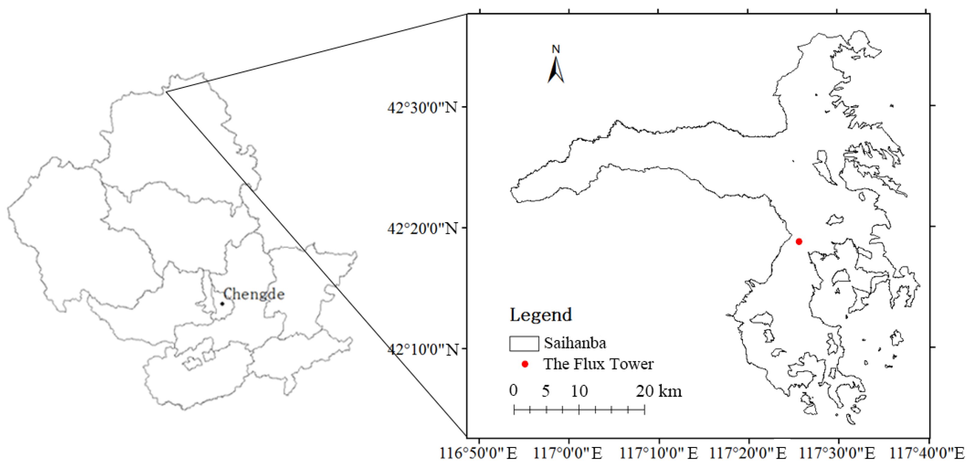
2.1. Study Area

The study area is located in Bashang area in the north of Chengde City, Hebei Province, China (latitude and longitude ranges: 42°04′~42°36′ N, 116°52′~117°39′ E). The main terrain is plateau platform, including grassland mountains, lakes and rivers, with an altitude of 1010~1939.9 m. The soil is mainly aeolian sandy soil, meadow soil, brown loam and grey forest soil [31,32]. The annual average temperature is −1.3 °C, and the annual average precipitation is 490 mm. The artificial afforestation area is 573.33 km2, and the natural forest area is 160 km2. The tree species are mainly northern Chinese larch (Larix principis-ruprechtii), camphor pine (Pinus sylvestris var. mongolica), spruce (Picea asperata) and silver birch (Betula platyphylla). The location of the study area is shown in Figure 1.

2.2. The Flux Tower

The flux tower of Saihanba mechanized forest farm is located in the northern Chinese larch plantation. The age of the stand was about 10 years by 2020. The flux tower is mainly composed of a vorticity correlation observation system and a micro-meteorological observation system. The vorticity correlation system is mainly composed of a three-dimensional ultrasonic anemometer and a fast response infrared CO2/H2O analyzer, which can measure wind speed, air temperature and air humidity. The micro-meteorological observation system includes anemometer, temperature and humidity sensor, net radiometer, total radiometer, barometer, rain gauge, soil temperature and humidity sensor, etc. The above instruments automatically collect and record data through the data collector and output the average value every 10 min.

2.3. Data and Preprocessing

2.3.1. Meteorological Data

The five meteorological data required for BEPS model are from the half-hour step data measured by the flux tower of Saihanba in 2020, which are temperature, radiation precipitation, wind speed and relative humidity. Because the study area is a small and medium-sized area, and there is only one flux tower for meteorological observation, the meteorological input data of the study area model is only from the flux tower. Due to extreme weather, routine instrument maintenance and special reasons (power failure, etc.), the original data usually needs to remove outliers and data interpolation.

2.3.2. Land Cover Type Data

When studying the regional-scale model, the land cover types in the study area were based on the vector data of Forest Resources Class II Survey in 2019. According to different land cover types, ArcGIS 10.0 software was used to generate the grid data of land cover types in the study area. The composition of tree species in the study area was relatively simple. The deciduous coniferous forest species was northern Chinese larch, the evergreen coniferous forest species included camphor pine and spruce, and the deciduous broad-leaved forest species was silver birch. Therefore, the land cover types in the study area were divided into eight types, as shown in Figure 2.

2.3.3. Leaf Area Index (LAI) Data

LAI is a key input data in BEPS model, which is closely related to photosynthesis, transpiration and productivity of vegetation [33]. Remote sensing technology is an important means to obtain forest LAI. In order to obtain high spatial-temporal resolution LAI data and reduce the impact of atmospheric and other factors, MODIS LAI data and Sentinel-2 remote sensing images were combined to generate time-series LAI data with a spatial resolution of 20 m and a time resolution of 8 days through remote sensing inversion and field verification.

2.3.4. ALOS Remote Sensing Image

Advanced Land Observing Satellite (ALOS) remote sensing image is provided by the Alaska Satellite Equipment Division of NASA (https://search.asf.alaska.edu/, accessed on 28 July 2023). The image processing process includes the following: (1) Projection conversion and resampling, changing the image projection mode to UTM projection, WGS84, and resampling the spatial resolution to 20 m. (2) Clipping, using the vector boundary of the study area to clip the image. (3) Stitching, stitching the trimmed images together to obtain DEM data of the study area. The preprocessed DEM data was used as the basis of the terrain data of the study area, and ArcGIS 10.0 software was used to generate the slope and aspect data of the study area, as shown in Figure 3.

2.3.5. MODIS NPP Data

The MODIS NPP product of the study area was obtained via NASA (http://ladsweb.modaps.eosdis.nasa.gov/, accessed on 1 October 2023), with a spatial resolution of 500 m and a temporal resolution of 8 days, a total of 46-time phases. The specific processing process included the following: (1) Change the image projection mode to UTM projection, WGS84 ellipsoid; (2) band combination; (3) the vector boundary was used to subset the data set; (4) add 46 images to get the annual NPP image data of the study area. The annual NPP image was used for the validation of model simulation.

2.4. Analysis of Influencing Factors

LAI and meteorological factors (temperature, radiation and precipitation) were selected as the main influencing factors [34,35], and the relative sensitivity analysis method was used to simulate the impact of different influencing factors on NPP in a certain range, while other input data remained unchanged. Because the meaning of temperature is high and low, the value of temperature cannot express the quantity, so only a simple analysis was made on the temperature. The sensitivity calculation formula of the influencing factor is as follows:
  S = i = 1 n 1 N P P i + 1 N P P i / N P P ¯ Q i + 1 Q i / Q ¯ n 1
where S is the sensitivity of a single factor, with a range of 0–1; N P P i + 1 , N P P i and N P P ¯ , respectively, represent the i + 1 and i times of simulation and the average value of both; Q i + 1 , Q i and Q ¯ , respectively, represent the value of the i + 1 and i times input factors and the average value of both, and n represents the number of changes of factors.
The study divided the S value into four levels, as shown in Table 1.

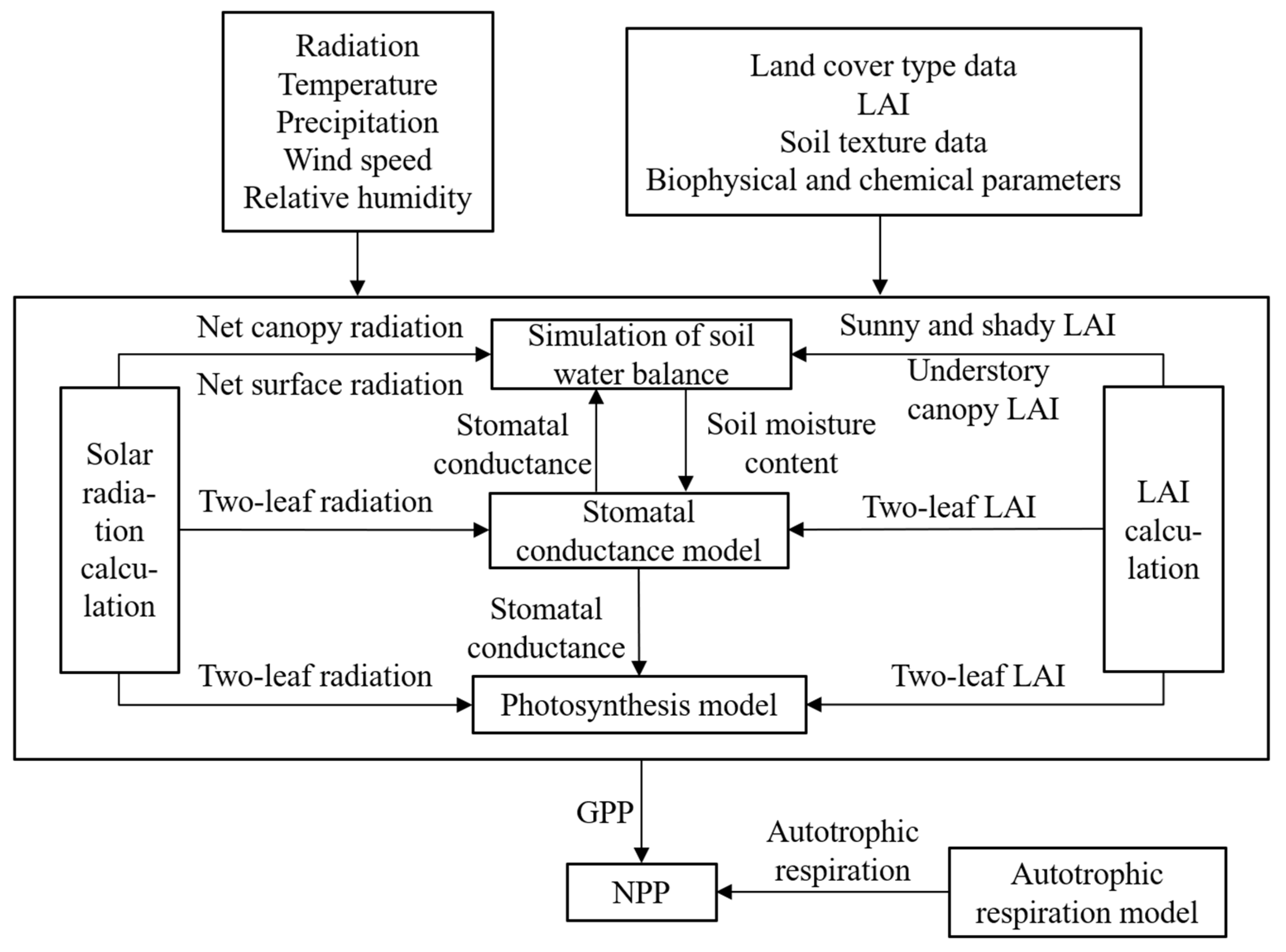
2.5. Model Description

Boreal Ecosystem Production Simulator (BEPS) model was first proposed by Liu et al. [14] in 1997 to simulate the NPP of northern forest ecosystem of Canada. Its daily step size is called BEPSDaily (BEPS at daily time steps). On the basis of BEPSDaily model, after gradual improvement, BEPSHourly (BEPS at hourly time steps) was developed. The simulation time step of the model is set to 30 min, the input data include meteorological data, vegetation type, canopy aggregation index, LAI, soil structure, etc., and the output results include GPP, NPP, latent heat flux and sensible heat flux, etc. The main steps of BEPSHourly model simulation and the relationship between sub models are shown in Figure 4.

2.5.1. Photosynthesis–Stomatal Conductance Model

The instantaneous photosynthetic rate at blade scale is calculated as follows:
A = min ( ω c , ω j ) R d
where A is the net photosynthetic rate. R d is the rate of photorespiration of vegetation. ω c and ω j represent the total photosynthetic rate affected by enzyme and electron transfer, respectively. ω c and ω j are calculated as follows:
ω c = a C i a d e C i + b = V c   m a x C i Γ C i + K c 1 +   [ O 2 ] K o
ω j = a C i a d e C i + b = J C i Γ 4 C i + 8 Γ
where V c   m a x is the maximum carboxylation rate. J is the electron transfer rate. [ O 2 ] is the concentration of intercellular O2. Γ Indicates the compensation point of CO2 without light respiration. C i is the intercellular CO2 concentration. K c and K o represent the Michaelis Menten coefficients of CO2 and O2, respectively.
C i = C s A g s
C s = C a A g b
g s = m × A × r h × f w 1 . 6 C s + b 1 . 6  
where C s and C a are leaf surface and atmospheric CO2 concentrations, respectively. g s and g b are CO2 conductivities from the inside of the cell to the leaf surface and from the leaf surface to the laminar boundary layer. b is the residual conductivity. f w is soil water availability. rh is the relative humidity.

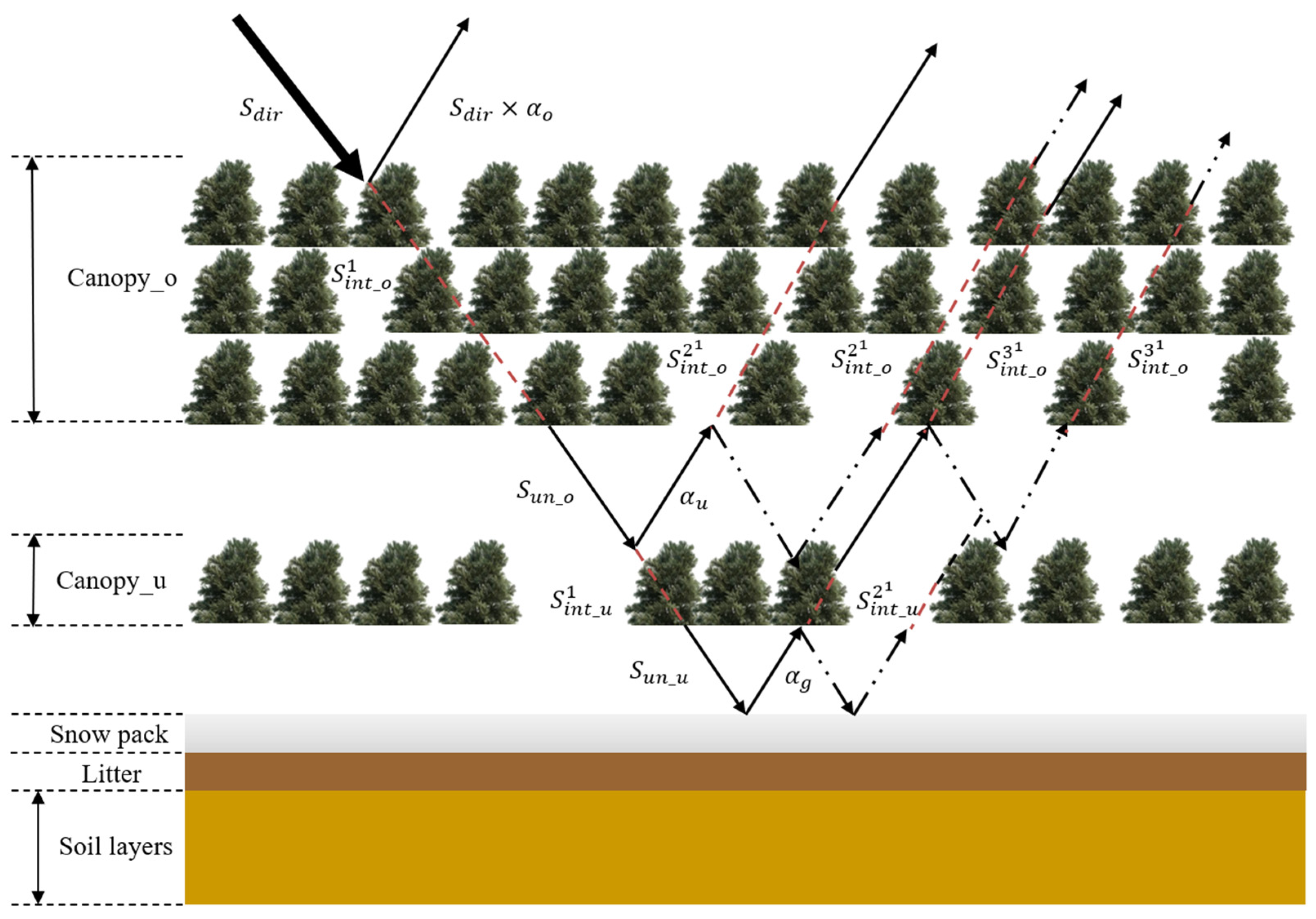
2.5.2. Radiative Transfer Model

In the traditional radiation transfer model of forest ecosystem, direct solar radiation is partially reflected through the overstory canopy, partially intercepted and absorbed by the overstory canopy, and the rest reaches the understory canopy. Part of the direct solar radiation received by the understory canopy is reflected from the understory canopy to the overstory canopy and fully absorbed. Part of the direct solar radiation received by the understory canopy is intercepted and absorbed by the understory canopy in the process of passing through the understory canopy, and the rest reaches the surface. Part of the direct solar radiation received by the surface is reflected to the understory canopy and fully absorbed.
The vegetation coverage in the study area is mostly deciduous forest. In winter, the radiation transmittance of the canopy is high, and the radiation reaching the surface accounts for a large proportion of the total solar radiation. Snow has high reflectivity, which makes the radiation reflected from the surface to the understory canopy layer larger in winter, so it is necessary to optimize the radiation transfer model. After optimization, most of the direct radiation reflected from the understory canopy layer to the overstory canopy layer enters the atmosphere through secondary transmission, and most of the direct radiation reflected from the surface to the understory canopy layer enters the atmosphere through secondary transmission to the overstory canopy layer, and then enters the atmosphere through secondary transmission to the overstory canopy layer, as shown in Figure 5.

2.5.3. Vegetation Autotrophic Respiration Model

Vegetative autotrophic respiration ( R a ) includes two parts: respiration for growth ( R g ) and respiration for maintaining basic metabolism ( R h ), including leaves, trunks, branches and roots, respectively:
R a = R g + R h
Generally speaking, plant growth respiration is not related to temperature, but only proportional to GPP:
R g = 0 . 2 × G P P
R h = i = 1 3 R i
where R i = l e a f , s t e m , r o o t is the maintenance respiration of leaves, branches and roots of vegetation, which is related to temperature:
R i = M i × γ i T
r i T = r i T 1 × Q 10 T T 1 10
where M i refers to the biomass of leaves, branches, trunks and roots of vegetation, respectively. γ i T is the respiration rate of various organs of vegetation at temperature T. Q 10 indicates the temperature coefficient, that is, the relative change of respiratory rate for every 10 °C change in temperature.
W i = k i × W 0
where W 0 refers to aboveground biomass. k l e a f is the ratio of the total biomass on the land occupied by leaves, k s t e m is the ratio of the total biomass on the land occupied by branches, and k r o o t is the ratio of underground to aboveground biomass.

2.5.4. Soil Moisture Balance Model

The premise of soil water content is to assume the balance of soil water content, and the calculation formula is as follows:
S o i l w a t e r = P g + S + P t E s T u T g
where S o i l w a t e r is the soil water content. P g is the ground precipitation. S is snow melting. P t is precipitation on trees. E s is soil evaporation. T u is under forest evapotranspiration. T g is canopy evapotranspiration.

2.5.5. Canopy Temperature Model

For the energy balance model of each part of the canopy, the components of the energy balance include transpiration latent heat, evaporation latent heat/sublimation latent heat, and sensible heat flux. Each component is brought into the energy balance equation to obtain the equation about the temperature of each part of the canopy:
Q = T × ρ a × C p × G h + V P D a i r × ρ a × C p × G w + G w w × X c l + G w w × X c s γ + ρ a × C p × × T × G w + G w w × X c l + G w w × X c s γ
T = T c T a = Q V P D a i r × ρ a × C p × G w + G w w × X c l + G w w × X c s / γ ρ a × C p × G h + × G w + G w w × X c l + G w w × X c s / γ
T c = T a + Q V P D a i r × ρ a × C p × G w + G w w × X c l + G w w × X c s / γ ρ a × C p × G h + × G w + G w w × X c l + G w w × X c s / γ
Stomatal conductance model is coupled with photosynthesis model and leaf energy balance model, which is solved iteratively by A, g s , C i , C s and T c .
Here, Q is the solar radiation absorbed by canopy leaves.   T c , T a and T are air temperature, temperature of each part of canopy and the difference between the two, respectively. ρ a is the air density. C p is the specific heat capacity of moist air. G h is the total heat conductance. V P D a i r is the differential saturation vapor pressure. G w and G w w are the total conductivity of water from inside of leaf to reference height and the total conductivity of water from leaf surface to reference height. X c l and X c s are the fraction of water covered canopy and the fraction of snow covered canopy. γ is the hygrometer constant. ∆ is the slope of saturated vapor pressure with temperature. A is the net photosynthetic rate. g s is the CO2 conductivities from the inside of the cell to the leaf surface. C i and C s are the intercellular CO2 concentration and the leaf surface CO2 concentration.

3. Results

3.1. Flux Tower Scale Simulation

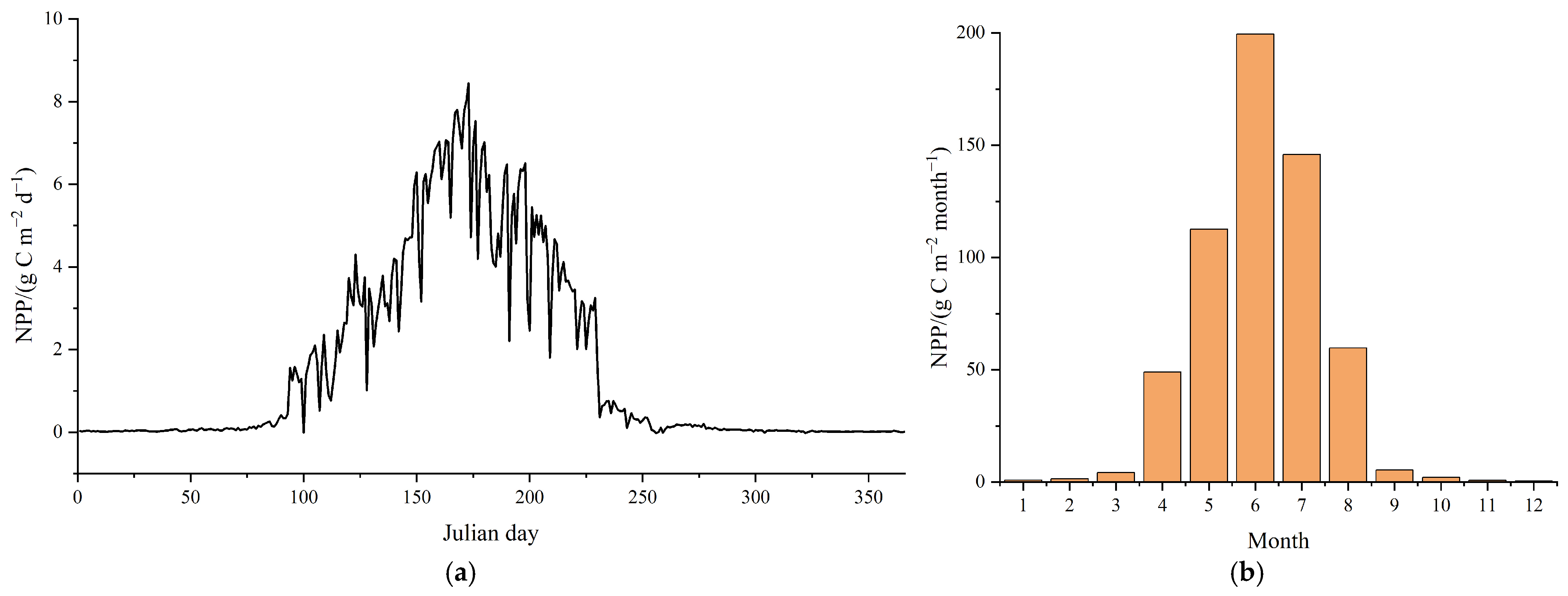
3.1.1. NPP Simulation

The daily NPP of northern Chinese larch showed a single peak trend, with a maximum value of 8.44 g C m−2 d−1 on 20 June, and basically 0 from January to March, November and December, as shown in Figure 6a. In 2020, the total NPP was the highest in June, which was 199.36 8.44 g C m−2, followed by July and May, which were between 100 and 200 g C m−2, and the remaining months were less than 100 g C m−2, as shown in Figure 6b. In 2020, the total NPP was 581.85 g C m−2, and the total NPP from May to July contributed 78.7% of the total annual NPP.

3.1.2. NPP Influencing Factors Analysis

An increase in LAI within a certain range would lead to an increase in solar radiation used in photosynthesis and the surface area of organs involved in photosynthesis, resulting in an increase in NPP. As the range of values of LAI varied from +50% to −50%, the results of NPP decreased accordingly from 767.94 g C m−2 a−1 to 342.81 g C m−2 a−1. The sensitivity of NPP to LAI was 0.722.
The increase in temperature would promote the growth of NPP, but there was a warming threshold. Heating up simultaneously affected photosynthesis and respiration, which in turn affected NPP. As the temperature changed from an increase of 5 +C to a decrease of 5 °C, the NPP results decreased accordingly from 636.93 g C m−2 a−1 to 470.40 g C m−2 a−1.
Radiation provided radiation energy for plant photosynthesis, serving as a signal to regulate several physiological processes of vegetation growth cycle, affecting transpiration of vegetation leaves, and thus affecting NPP. As the range of values of radiation varied from +50% to −50%, the results of NPP decreased accordingly from 624.96 g C m−2 a−1 to 469.63 g C m−2 a−1. The sensitivity of NPP to radiation was 0.233.
Water was a necessary condition for various physiological activities of vegetation. It controlled the opening and closing of stomata and was also a means of transporting plant nutrients. Low or high precipitation would limit vegetation growth. As the range of values of precipitation varied from +50% to −50%, the results of NPP remained virtually unchanged. The sensitivity of NPP to precipitation was 0.0004. The sensitivity levels of NPP influencing factors were shown in Table 2.

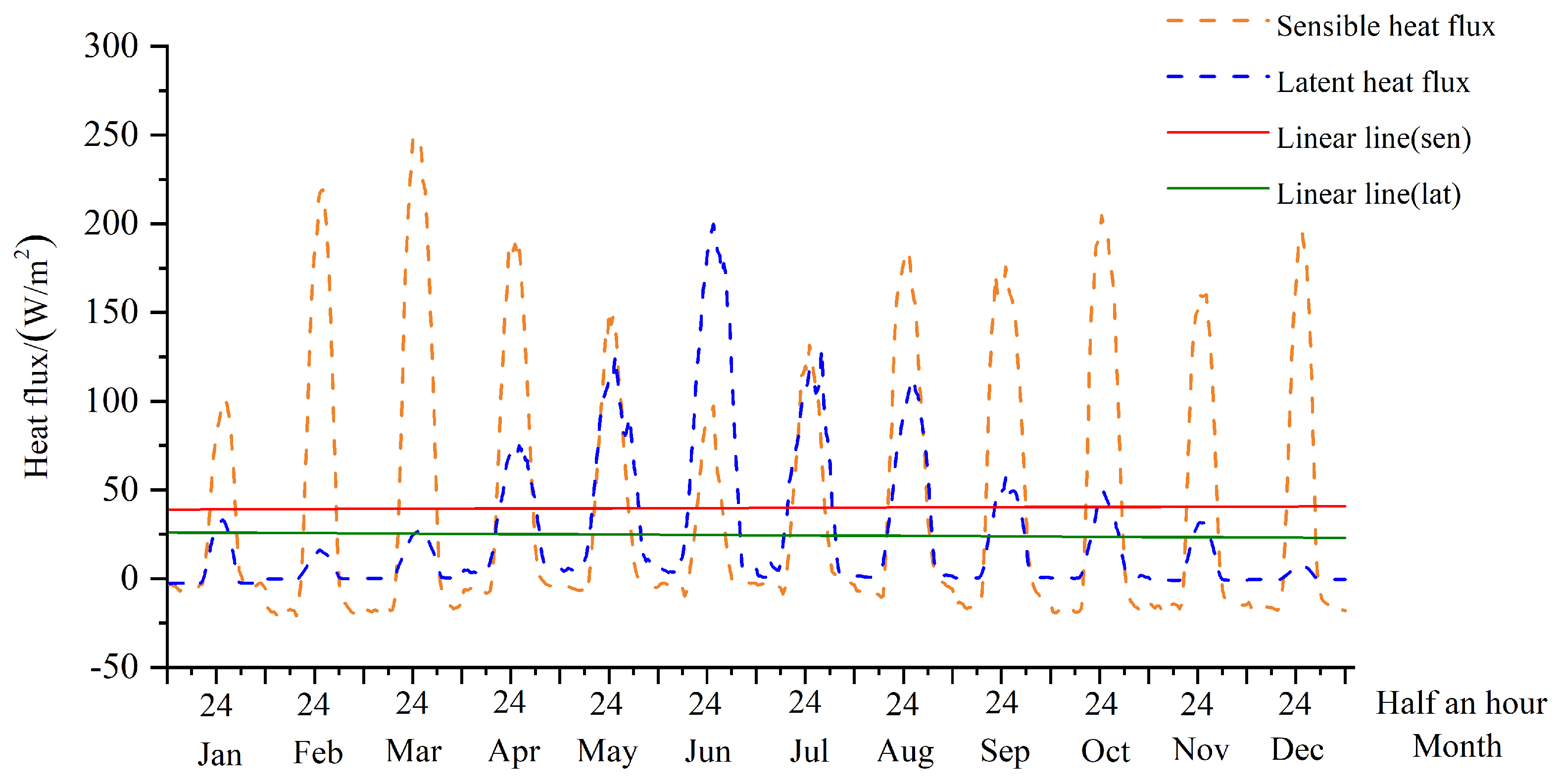
3.1.3. Simulation of Latent and Sensible Heat Fluxes

It can be seen from Figure 7 that the monthly average diurnal variations of latent heat flux and sensible heat flux were both single peak curves, reaching the maximum at noon and lowest at night. Compared with sensible heat flux, the seasonal variation of latent heat flux was more significant, and it was higher in summer vegetation growing season than in non-growing season. The sensible heat flux was higher from February to April and from August to December, and was in a low peak state during the vigorous vegetation period. The monthly average peak of latent heat flux reached the maximum in June, which was 199.98 W/m2, and the monthly average peak of sensible heat flux reached the maximum in March, which was 247.31 W/m2.

3.1.4. Canopy Temperature Simulation

It can be seen from Figure 8 that during the day, the change of overstory canopy temperature was consistent with that of air temperature. The temperature of overstory canopy was slightly higher than that of air during the day, but it was the opposite at night. The understory canopy temperature was significantly higher than the overstory canopy temperature and air temperature at 0–8, basically equal at 8–10, and slightly higher at 10–24. In 2020, the average air temperature of the flux tower was 1 °C, the average temperature of the overstory canopy was 1.1 °C, and the average temperature of the understory canopy was 3.6 °C.

3.2. Regional Scale Simulation

3.2.1. Simulation Results

In 2020, the total NPP in the study area was 4.25 × 10¹¹ g C a−1, with an average of 564.71 g C m−2 a−1. The annual NPP and average NPP of different stand types were different (Table 3). The stand type with the largest average NPP was silver birch, which was 647.84 g C m−2 a−1, followed by coniferous and broad-leaved mixed forest, camphor pine, spruce, evergreen and deciduous coniferous forest, northern Chinese larch, sparse forest and shrub forest. The total NPP was related to the area of the stand type. Because northern Chinese larch was widely planted, the stand type with the largest total NPP was northern Chinese larch, which was 1.73 × 10¹¹ g C a−1, followed by silver birch, camphor pine, coniferous and broad-leaved mixed forest, spruce, sparse forest and shrub forest, evergreen and deciduous coniferous forest. It can be seen that for the primary productivity of each stand type in the study area, broad-leaved forest > coniferous and broad-leaved mixed forest > coniferous forest, evergreen forest > deciduous forest.
As can be seen from Figure 9, the NPP in the study area in 2020 was mainly concentrated in 300~700 g C m−2 a−1, and in a few area it was below 300 g C m−2 a−1, and in some areas it reached more than 700 g C m−2 a−1. The quality of forest land in the eastern part of the study area was high, and its annual average NPP was generally higher than 700 g C m−2 a−1.

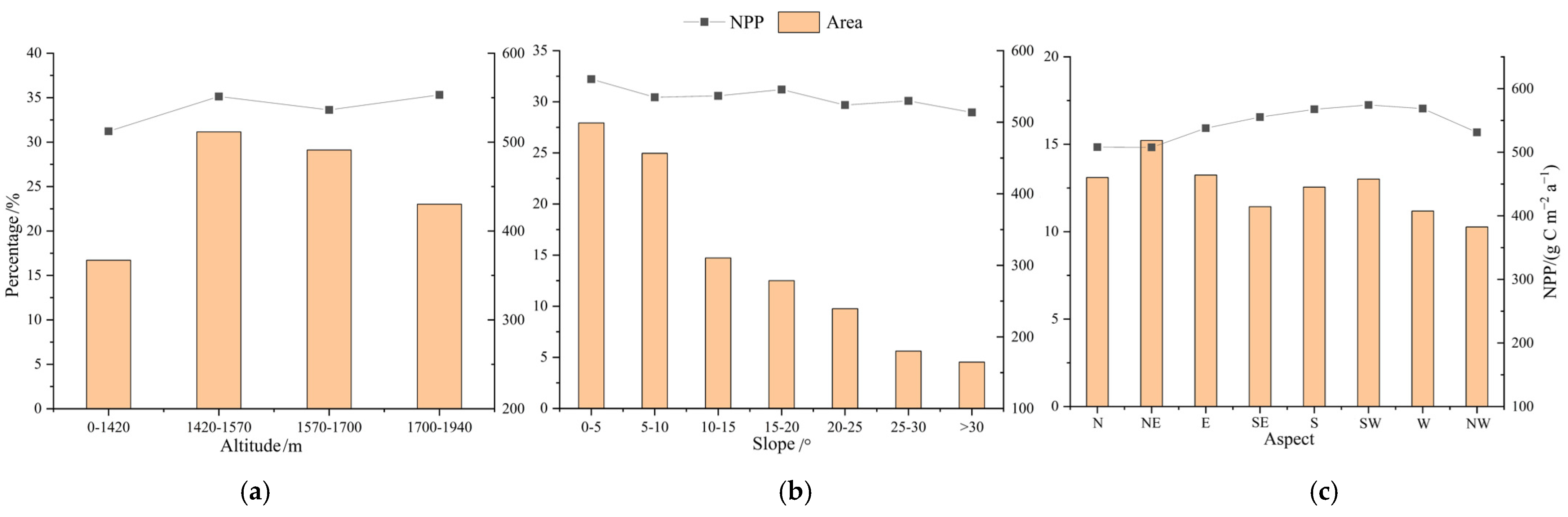
3.2.2. Analysis of the Impact of Topographic Factors on NPP

  • Altitude
The average value of NPP in the study area basically fluctuated up and down with altitude, ranging from 512 to 554 g C m−2 a−1, with a small variation range, as shown in Figure 10a.
2.
Slope
The average value of NPP in the study area showed a decreasing trend with the increase of altitude. When the slope was within the range of 0~5°, the average value of NPP was the largest, which was 560.24 g C m−2 a−1. When the slope was greater than 30°, the average value of NPP was the lowest, which was 513.77 g C m−2 a−1, as shown in Figure 10b.
3.
Aspect
The average NPP values of the northeast slope, the east slope and the north slope were higher, reaching 565–575 g C m−2 a−1, as shown in Figure 10c. The average NPP values of the south slope and the southwest slope were the lowest, reaching 508 g C m−2 a−1. NPP was generally affected by slope aspect as follows: shady slope > sunny slope.

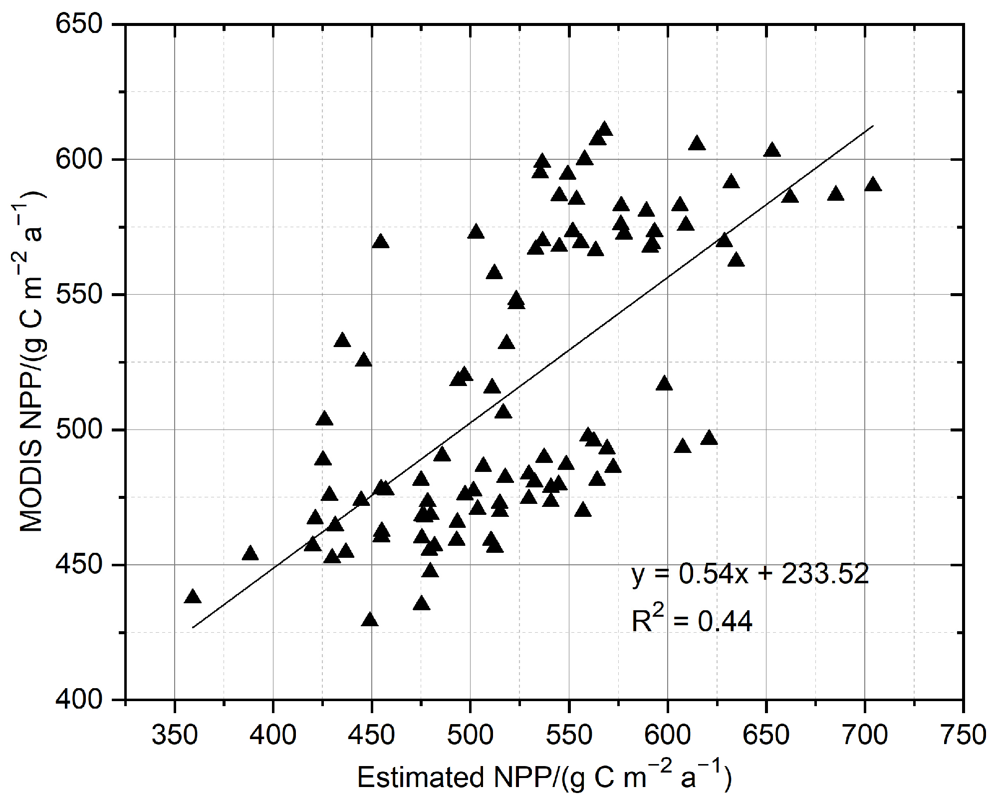
3.2.3. Validation of Estimated NPP

The NPP of the study area in 2020 obtained in this study was basically consistent with the MODIS NPP data products. The NPP of the study area estimated by BEPSHourly ranged from 13.14 to 1117.26 g C m−2 a−1, with an average of 564.71 g C m−2 a−1. MODIS NPP values ranged from 270 to 811 g C m−2 a−1, with an average of 503.96 g C m−2 a−1. As can be seen from Figure 11, the NPP estimated in this study had a good correlation with MODIS NPP. The R2 of the regression equation between MODIS NPP and estimated NPP was 0.44.

4. Discussion

4.1. Diurnal and Seasonal Variations of Latent and Sensible Heat Fluxes

During the course of one day, the latent heat flux became positive at about 6:00, that is, there was a sharp increase in the amount of heat energy dissipated by evaporation. By 13:00, the latent heat flux reached its maximum value, which was due to the rapid increase in latent heat flux values during the day because of the fast temperature rise, strong turbulence and strong ground evaporation and plant transpiration. After 13:00, although the air temperature was still high, the latent heat flux had a sharp decrease. Zhou [36] suggested that one of the reasons for this was that the stomata on the leaf surfaces of the trees closed after the high temperature at 14:00, and transpiration decreased. The latent heat flux only became negative after 20:00, when evapotranspiration stopped and water vapor released heat to the ground through condensation. At night, due to low temperature, weakened turbulence, reduced evaporation and basic cessation of plant transpiration, the absolute value of latent heat flux was smaller and less variable. As for the sensible heat flux from the daily process, the minimum value appeared in the night and was negative, while the maximum value generally appeared from 12:00 to 14:00. This was due to the sensible heat flux of energy coming from the radiant energy, the radiation being the largest before and after noon, the presence of the forest canopy layer increasing the turbulence of the exchange. At night, the forest canopy absorbed heat from the atmosphere by turbulent exchange as the long-wave radiation from the canopy layer lost heat.
The latent heat flux and sensible heat flux of the forest in the study area had obvious seasonal variations [34]. In the growing season, the latent heat flux was larger than the sensible heat flux and dominated, and the forest evapotranspiration dissipated a large amount of latent heat flux. The latent heat flux reached a maximum in June, mainly because the forest growth was in the most vigorous stage, the LAI had reached the maximum value, and there was sufficient rainfall. The leaves began to fall off in September, and the latent heat flux showed a gradual decreasing tendency. In the non-growing season, most of the energy was allocated to the sensible heat flux, which was higher than the latent heat flux, when the evapotranspiration of the forest was small [37].

4.2. The Influence of Slope Aspect on Forest Growth

Some studies have shown that compared with the shady slope, the growth of forest vegetation was better on the sunny slope. This was because there was more light on the sunny slope than on the shady slope. Light has a positive effect on the distribution and productivity of forest vegetation and promotes the growth of forest vegetation. Qi [38] showed that in the Daxing’an Mountains, sunny slope can promote the growth of forest vegetation. Xiong et al. [39] found that the carbon storage and NPP of forest vegetation on Fanjing Mountain in Guizhou Province were higher on sunny slope than on shady slope.
Other studies have shown that forest vegetation grew better on shady slope than on sunny slope. This was because the light intensity on shady slopes was lower than that on sunny slopes. In order to improve their physiological metabolic activities, forest vegetation photosynthetic efficiency on shady slope was higher than that on sunny slope, and vegetation growth was more vigorous than that on sunny slope. This study showed that the NPP of Saihanba mechanized forest farm was higher on the shady slope than on the sunny slope. Yang et al. [40] found that the LAI of different forest types (coniferous forest, broad-leaved forest, coniferous broad-leaved mixed forest) in Saihanba area was higher on shady slope than on sunny slope. In Taiyue Mountain, Yi [41] found that the forest carbon density was higher on the shady slope and lower on the sunny slope. It was considered that the climate in the north was dry and the water evaporation on the shady slope was less than that on the sunny slope, which was conducive to water conservation and vegetation growth. The solar radiation intensity of shady slope was less than that of sunny slope, the water evaporation was slower, and the soil moisture was more conducive to the growth of vegetation. The precipitation in northern China was relatively insufficient, and it was more conducive to reduce water evaporation on shady slopes, and the available water of forest vegetation was more than that on sunny slopes. In this study, the altitude of the study area was 1000–1940 m, the sunshine was strong in summer, the precipitation was rare, and the water evaporation on the sunny slope was higher than that on the shady slope. Therefore, the NPP on the shady slope of the study area was higher than that on the sunny slope.

4.3. Simulation of Forest NPP

In the study area, northern Chinese larch plantation covered the largest area, so in the study of forest NPP, most of the research objects were northern Chinese larch. There were many factors affecting forest NPP, such as age, initial planting density, stand structure and so on. Zhao et al. [42] found that the productivity of northern Chinese larch was different at different ages, with a minimum of 3.22 m3 hm−2 a−1 and a maximum of 5.72 m3 hm−2 a−1. Hu et al. [43] found that the annual average net productivity of coniferous and broad-leaved mixed forests in different site types was different. The lowest value appeared in the forest types with poor site and coniferous broad-leaved ratio of 2:1, which was 4.36 t hm−2 a−1, and the maximum value appeared in the forest types with better site and coniferous broad-leaved ratio of 1:2, which was 9.58 t hm−2 a−1. The result of this study was that the NPP of the forest in the study area was 564.71 g C m−2 a−1, which was consistent with the above results.
NPP simulation results of coniferous forest, broad-leaved forest and coniferous broad-leaved mixed forest by different researchers using different models were summarized, as shown in Table 4. The NPP range of coniferous forest simulated by different researchers was 345–585 g C m−2 a−1, the broad-leaved forest was 624–870 g C m−2 a−1, and the coniferous and broad-leaved mixed forest was 423–928 g C m−2 a−1. The simulation results of this study were within the above ranges. The simulation of vegetation NPP can be affected by tree species composition, different years, geographical location, model adoption, data sources and simulation accuracy.

4.4. Limitations and Direction of Improvements

There was only one flux tower in the study area. Whether its data can cover the whole study area remains to be studied. Since there was no field measurement of NPP, the results of this study were only verified and compared with MODIS NPP and other research results. Other studies [15,47,48] have found that LAI was an important input data of the model, and its accuracy would affect some components of the model, including photosynthesis and vegetation respiration. Therefore, high-precision LAI data was a necessary condition for reliable simulation results. In the future, the accuracy of the results of this study can be improved by improving the above aspects.

5. Conclusions

In this study, we used BEPSHourly model to estimate the NPP of the study area in 2020, analyzed the factors affecting the NPP, and verified the results with MODIS NPP. At the same time, forest latent and sensible heat flux and canopy temperature were simulated. The results showed that within the scale of the flux tower, NPP reached a maximum of 0.33 g C m−2 (0.5 h)−1 in June. Sensitivity analysis showed that NPP was highly sensitive to the change of LAI. Latent heat flux and sensible heat flux showed different seasonal variations. Canopy temperature of the upper forest maintained the consistency of change with air temperature. At the regional scale, the total NPP in the study area in 2020 was 4.25 × 10¹¹ g C a−1, with an average of 564.71 g C m−2 a−1. The annual average NPP of silver birch was the largest, and the total NPP of northern Chinese larch was the largest. The spatial distribution of NPP was affected by topographic factors. This study contributes new aspects to our understanding of the application of the model, helping to improve the accuracy of NPP estimation in future research.

Author Contributions

Conceptualization, Z.Y. and W.L.; methodology, W.L.; software, Z.Y. and L.H.; validation, Z.Y. and Y.Q.; formal analysis, Z.Y.; investigation, Z.Y., H.L. and L.H.; resources, X.H.; data curation, Z.Y., Y.Q., H.L. and W.L.; writing—original draft preparation, Z.Y.; writing—review and editing, X.H. and W.L.; supervision, X.H. and W.L.; project administration, X.H. and W.L.; funding acquisition, X.H. and W.L. All authors have read and agreed to the published version of the manuscript.

Funding

This research was funded by “National Natural Science Foundation of China (Grant number 31700561)” and the National Key R&D Program of China (Grant number 2022YFD2200503).

Institutional Review Board Statement

Not applicable.

Informed Consent Statement

Not applicable.

Data Availability Statement

All data generated or analyzed during this study are included in this published article.

Acknowledgments

Special thanks need to go to the Saihanba Mechanized Forest Farm for providing the forest inventory data.

Conflicts of Interest

The authors declare no conflicts of interest.

References

  1. Feng, X.; Liu, G.; Chen, J.; Chen, M.; Liu, J.; Ju, W.; Sun, R.; Zhou, W. Net primary productivity of China’s terrestrial ecosystems from a process model driven by remote sensing. J. Environ. Manag. 2007, 85, 563–573. [Google Scholar] [CrossRef]
  2. Li, X.; Du, H.; Mao, F.; Zhou, G.; Han, N.; Xu, X.; Liu, Y.; Zhu, D.; Zheng, J.; Dong, L.; et al. Assimilating spatiotemporal MODIS LAI data with a particle filter algorithm for improving carbon cycle simulations for bamboo forest ecosystems. Sci. Total Environ. 2019, 694, 133803.1–133803.14. [Google Scholar] [CrossRef]
  3. Pelt, R.; Sillett, S.; Kruse, W.; Freund, J.; Kramer, R. Emergent crowns and light-use complementarity lead to global maximum biomass and leaf area in Sequoia sempervirens forests. For. Ecol. Manag. 2016, 375, 279–308. [Google Scholar] [CrossRef]
  4. Le Toan, T.; Quegan, S.; Davidson, M.; Balzter, H.; Paillou, P.; Papathanassiou, K.; Plummer, S.; Rocca, F.; Saatchi, S.; Shugart, H. The BIOMASS mission: Mapping global forest biomass to better understand the terrestrial carbon cycle. Remote Sens. Environ. 2011, 115, 2850–2860. [Google Scholar] [CrossRef]
  5. Xue, M.; Chen, Y.; Jia, L.; Wang, X.; Yan, M.; Tian, X. Estimation of net primary productivity by beps model-a case study in fujian province. In Proceedings of the 2017 IEEE International Geoscience and Remote Sensing Symposium (IGARSS), Fort Worth, TX, USA, 23–28 July 2017; pp. 6213–6216. [Google Scholar] [CrossRef]
  6. Running, S.; Coughlan, J. A general model of forest ecosystem processes for regional applications I. Hydrologic balance, canopy gas exchange and primary production processes. Ecol. Model. 1988, 42, 125–154. [Google Scholar] [CrossRef]
  7. Lieth, H. Primary Productivity of the Biosphere; Whittaker, R., Ed.; Spring: New York, NY, USA, 1975. [Google Scholar]
  8. Wang, Z.; Zhou, Y.; Sun, X.; Xu, Y. Estimation of NPP in Huangshan district based on deep learning and CASA model. Forests 2024, 15, 1467. [Google Scholar] [CrossRef]
  9. Sallaba, F.; Lehsten, D.; Seaquist, J.; Sykes, M. A rapid NPP meta-model for current and future climate and CO2 scenarios in Europe. Ecol. Model. 2015, 302, 29–41. [Google Scholar] [CrossRef]
  10. Canadell, J.; Mooney, H.; Baldocchi, D.; Berry, J.; Ehleringer, J.; Field, C.; Gower, S.; Hollinger, D.; Hunt, J.; Jackson, R.; et al. Carbon metabolism of the terrestrial biosphere: A multi-technique appraoch for improved understanding. Ecosystems 2000, 3, 115–130. [Google Scholar] [CrossRef]
  11. Wang, B.; Li, M.; Fan, W.; Zhang, F. Quantitative simulation of C budgets in a forest in Heilongjiang province, China. iForest—Biogeosci. For. 2016, 10, 128–135. [Google Scholar] [CrossRef]
  12. Liu, J.; Chen, J.; Cihlar, J.; Chen, W. Net Primary Productivity Mapped for Canada at 1-km Resolution. Glob. Ecol. Biogeogr. 2002, 11, 115–129. [Google Scholar] [CrossRef]
  13. Zhang, S.; Zhang, J.; Bai, Y.; Kojo, U.; Igbawua, T.; Chang, Q.; Zhang, D.; Yao, F. Evaluation and improvement of the daily boreal ecosystem productivity simulator in simulating gross primary productivity at 41 flux sites across Europe. Ecol. Model. 2018, 368, 205–232. [Google Scholar] [CrossRef]
  14. Liu, J.; Chen, J.; Cihlar, J.; Park, W. A process-based boreal ecosystem productivity simulator using remote sensing inputs. Remote Sens. Environ. 1997, 62, 158–175. [Google Scholar] [CrossRef]
  15. Kojo, U.; Zhang, J.; Maharjan, S.; Bai, Y.; Zhang, S.; Yao, F. Analysis of spatiotemporal dynamics of forest Net Primary Productivity of Nepal during 2000–2015. Int. J. Remote Sens. 2020, 41, 4336–4364. [Google Scholar] [CrossRef]
  16. Guan, D.; Nie, J.; Zhou, L.; Chang, Q.; Cao, J. How to simulate carbon sequestration potential of forest vegetation? A forest carbon sequestration model across a typical mountain city in China. Remote Sens. 2023, 15, 5096. [Google Scholar] [CrossRef]
  17. Holdridge, L. Determination of world plant formations from simple climatic data. Science 1947, 105, 367–368. [Google Scholar] [CrossRef]
  18. Woodward, F.; Williams, B. Climate and plant distribution at global and local scales. Vegetatio 1987, 69, 189–197. [Google Scholar] [CrossRef]
  19. Neilson, R. A Model for Predicting Continental-Scale Vegetation Distribution and Water Balance. Ecol. Appl. 1995, 5, 362–385. [Google Scholar] [CrossRef]
  20. Delire, C.; Foley, J.; Thompson, S. Evaluating the carbon cycle of a coupled atmosphere-biosphere model. Glob. Biogeochem. Cycles 2003, 17, 1012. [Google Scholar] [CrossRef]
  21. Kucharik, C.; Barford, C.; Maayar, M.; Wofsy, S.; Monson, R.; Baldocchi, D. A multiyear evaluation of a Dynamic Global Vegetation Model at three AmeriFlux forest sites: Vegetation structure, phenology, soil temperature, and CO2 and H2O vapor exchange. Ecol. Model. 2006, 196, 1–31. [Google Scholar] [CrossRef]
  22. Xie, X.; Li, A.; Jin, H. The simulation models of the forest carbon cycle on a large scale: A review. Acta Ecol. Sin. 2018, 38, 41–54. [Google Scholar] [CrossRef]
  23. Kucharik, C.; Foley, J.; Delire, C.; Fisher, V.; Coe, M.; Lenters, J.; Young-Molling, C.; Ramankutty, N.; Norman, J.; Gower, S. Testing the performance of a dynamic global ecosystem model: Water balance, carbon balance, and vegetation structure. Glob. Biogeochem. Cycles 2000, 105, 795–825. [Google Scholar] [CrossRef]
  24. Potter, C.; Randerson, J.; Field, C.; Matson, P.; Vitousek, P.; Mooney, H.; Klooster, S. Terrestrial ecosystem production: A process model based on global satellite and surface data. Glob. Biogeochem. Cycles 1993, 7, 811–841. [Google Scholar] [CrossRef]
  25. Parton, W.; Stewart, J.; Cole, C. Dynamics of C, N, P and S in grassland soils: A model. Biogeochemistry 1988, 5, 109–131. [Google Scholar] [CrossRef]
  26. Farquhar, G.; Caemmerer, S.; Berry, J. A biochemical model of photosynthetic CO2 assimilation in leaves of C3 species. Planta 1980, 149, 78–90. [Google Scholar] [CrossRef]
  27. Matsushita, B.; Chen, J.; Kameyama, S.; Tamura, M. Estimation of net primary productivity using Boreal Ecosystem Productivity Simulator—A case study for Hokkaido Island, Japan. In Proceedings of the IEEE Transactions on International Geoscience and Remote Sensing Symposium, Toronto, ON, Canada, 24–28 June 2002; pp. 2346–2348. [Google Scholar] [CrossRef]
  28. Higuchi, K.; Shashkov, A.; Chan, D.; Saigusa, N.; Murayama, S.; Yamamoto, S.; Kondo, H.; Chen, J.; Liu, J.; Chen, B. Simulations of seasonal and inter-annual variability of gross primary productivity at Takayama with BEPS ecosystem model. Agric. For. Meteorol. 2005, 134, 143–150. [Google Scholar] [CrossRef]
  29. Zhou, Y.; Zhu, Q.; Chen, J.; Wang, Y.; Liu, J.; Sun, R.; Tang, S. Observation and simulation of net primary productivity in Qilian Mountain, western China. J. Environ. Manag. 2007, 85, 574–584. [Google Scholar] [CrossRef]
  30. Fu, Y.; Tian, D.; Hou, Z.; Wang, M.; Zhang, N. Review on the evaluation of global forest carbon sink function. J. Beijing For. Univ. 2022, 44, 1–10. [Google Scholar] [CrossRef]
  31. Tan, W.; Zhou, L.; Liu, K. Soil aggregate fraction-based 14C analysis and its application in the study of soil organic carbon turnover under forests of differents ages. Chin. Sci. Bull. 2013, 58, 1936–1947. [Google Scholar] [CrossRef]
  32. Yang, H. Assessment on Plantation Forest Visual Resource of Saihanba Mechanical Plantation. Ph.D. Thesis, Hebei Agricultural University, Baoding, China, 2017. [Google Scholar]
  33. Xiao, F.; Zhang, Q.; Fan, S. Progress of research on carbon fixation and storage of forest ecosystems in China. World For. Res. 2006, 19, 53–57. [Google Scholar] [CrossRef]
  34. Lu, W. Research on Parameter Optimization and Application of Forest Carbon Cycle Model(BEPS) at Hourly Time Steps. Ph.D. Thesis, Northeast Forestry University, Harbin, China, 2016. [Google Scholar]
  35. Mao, X. Study on the Model of Northeast Forest Carbon Cycle at Daily Step and the Integrated Application of Remote Sensing. Ph.D. Thesis, Northeast Forestry University, Harbin, China, 2011. [Google Scholar]
  36. Zhou, M. Research on the Hydrological Process and Laws of Larix Gmelini Ecosystem at the Greater Xingan Mountains. Ph.D. Thesis, Beijing Forestry University, Beijing, China, 2003. [Google Scholar]
  37. Zhang, Y. Energy and Water Budget of a Poplar Plantation in Suburban Beijing. Ph.D. Thesis, Beijing Forestry University, Beijing, China, 2010. [Google Scholar]
  38. Qi, Y. Estimates of Forest Above Ground Carbon Storage Using Remote Sensing in Daxing’an Mountains. Ph.D. Thesis, Northeast Forestry University, Harbin, China, 2014. [Google Scholar]
  39. Xiong, H.; YU, F.; Gu, X.; Wu, X. Biomass, net production, carbon storage and spatial distribution features of different forest vegetation in Fanjing Mountains. Ecol. Environ. Sci. 2021, 30, 264–273. [Google Scholar] [CrossRef]
  40. Yang, H.; Peng, B.; Fan, H.; Gu, J.; Li, R.; Li, W. Study on relationship of topographic factors and leaf area index in different forest type. J. Hebei For. Sci. Technol. 2018, 3, 1–6. [Google Scholar] [CrossRef]
  41. Yi, F. Study on forest carbon density and spatial distribution parttern of Taiyue Mountain in Shanxi Province. J. Shanxi Agric. Sci. 2017, 45, 1814–1817. [Google Scholar] [CrossRef]
  42. Zhao, K.; Wang, L.D.; Wang, L.; Jia, Z.; Ma, L. Stock volume and productivity of Larix principis-rupprechtii in northern and northwestern China. J. Beijing For. Univ. 2015, 37, 24–31. [Google Scholar] [CrossRef]
  43. Hu, J.; Yang, B.; Xu, S. Enhancing carbon sink capacity and promoting green development—Carbon sink change of Saihanba mechanized forest farm based on FORECAST model. For. Sci. Technol. 2023, 48, 48–51. [Google Scholar] [CrossRef]
  44. Tao, B.; Li, K.; Shao, X.; Cao, M. Temporal and spatial pattern of net primary production of terrestrial ecosystems in China. Acta Geogr. Sin. 2003, 58, 372–380. [Google Scholar] [CrossRef]
  45. Liu, M. Land-Use/Land-Cover Change and Terrestrial Ecosystem Phytomass Carbon Pool and Production in China. Ph.D. Thesis, Chinese Academy of Sciences, Beijing, China, 2001. [Google Scholar]
  46. Zhu, W.; Pan, Y.; Zhang, J. Estimation of net primary productivity of Chinese terrestrial vegetation based on remote sensing. Acta Plytoecol. Sin. 2007, 31, 413–424. [Google Scholar] [CrossRef]
  47. Mao, F.; Du, H.; Zhou, G.; Li, X.; Xu, X.; Li, P.; Sun, S. Coupled LAI assimilation and BEPS model for analyzing the spatiotemporal pattern and heterogeneity of carbon fluxes of the bamboo forest in Zhejiang Province, China. Agric. For. Meteorol. 2017, 242, 96–108. [Google Scholar] [CrossRef]
  48. Ge, Z.; Guo, H.; Zhao, B.; Zhang, C.; Peltola, H.; Zhang, L. Spatiotemporal patterns of the gross primary production in the salt marshes with rapid community change: A coupled modeling approach. Ecol. Model. 2016, 321, 110–120. [Google Scholar] [CrossRef]
Figure 1. Location of the study area and the flux tower.
Applsci 14 10912 g001
Figure 2. Land cover types.
Applsci 14 10912 g002
Figure 3. Topographic factor maps of the study area: (a) DEM data; (b) the slope map; (c) the slope aspect map.
Applsci 14 10912 g003
Figure 4. Model structural theory process.
Applsci 14 10912 g004
Figure 5. Schematic diagram of radiation transmission.
Applsci 14 10912 g005
Figure 6. Simulated NPP of the flux tower in 2020: (a) Daily NPP; (b) monthly NPP.
Applsci 14 10912 g006
Figure 7. Monthly averaged daily variation of simulated heat flux of the flux tower.
Applsci 14 10912 g007
Figure 8. Annual average daily variation of air temperature and simulated canopy temperature of the flux tower.
Applsci 14 10912 g008
Figure 9. NPP distribution of the study area in 2020.
Applsci 14 10912 g009
Figure 10. Impact of topographic factors on NPP. (a) Altitude; (b) slope; (c) aspect.
Applsci 14 10912 g010
Figure 11. Regression analysis of estimated and MODIS NPP.
Applsci 14 10912 g011
Table 1. Sensitivity level division.
LevelValue of SMeaning
I0 ≤ S ≤ 0.1Insensitive
II0.1 < S ≤ 0.25Slight Sensitive
III0.25 < S ≤ 0.5Medium Sensitive
IV0.5 < S ≤ 1Highly Sensitive
Table 2. Sensitivity level classification statistics.
Influencing FactorSensitivityLevel
LAI0.722IV
Radiation0.233II
Precipitation0.0004I
Table 3. NPP statistics of different stand types.
Stand TypeAnnual NPP
(g C m−2 a−1)
Total NPP
(g C a−1)
Northern Chinese Larch518.051.73 × 1011
Camphor Pine576.957.81 × 1010
Spruce565.481.95 × 1010
Silver Birch647.841.22 × 1011
Coniferous and Broad-leaved Mixed Forest661.352.52 × 1010
Evergreen and Deciduous Coniferous Forest558.052.46 × 109
Sparse Forest and Shrub Forest292.605.11 × 109
Table 4. Comparison of NPP results for different studies (g C m−2 a−1).
Stand TypeThis StudyTao [44] Liu [45]Zhu [46]
Coniferous Forest518.05–576.95345585447
Broad-leaved Forest647.84624870643
Coniferous and Broad-leaved Mixed Forest661.35423928469
Disclaimer/Publisher’s Note: The statements, opinions and data contained in all publications are solely those of the individual author(s) and contributor(s) and not of MDPI and/or the editor(s). MDPI and/or the editor(s) disclaim responsibility for any injury to people or property resulting from any ideas, methods, instructions or products referred to in the content.

