Article

Artificial Intelligence for Earthquake Prediction: A Preliminary System Based on Periodically Trained Neural Networks Using Ionospheric Anomalies

Department of Cartographic Engineering, Geodesy and Photogrammetry, Universitat Politècnica de València, Camino de Vera s/n, 46022 Valencia, Spain
Appl. Sci. 2024, 14(23), 10859; https://doi.org/10.3390/app142310859
Submission received: 18 October 2024 / Revised: 19 November 2024 / Accepted: 20 November 2024 / Published: 23 November 2024
(This article belongs to the Special Issue Artificial Intelligence for Earthquake Prediction)

Abstract

:
There is increasing evidence that anomalies in the ionosphere could appear a few days before large earthquakes. Many significant successes with using anomalies for predictions have been reported, although they are usually limited, both in space, to a specific geographic area, and in time, to one or a few events. To date, no solution has been presented that consistently yields the location and magnitude of future earthquakes and thus can be used to develop a warning service. The purpose of this research is to improve on the possible use of Global Ionospheric Maps for earthquake prediction. The use of three-dimensional data matrices, having spatiotemporal information to feed a convolutional neural network, is proposed in this contribution. This network was trained on all large earthquakes occurring from the beginning of the year 2011 to the beginning of October 2024 but it is proposed that it be periodically retrained with new data. This network has reached an accuracy of around 60% in the validation data for a division into eight categories of different earthquake magnitudes. Nevertheless, this percentage increases considerably if the classification into neighboring categories is also accepted, something that could be clearly admissible for the purposes of a warning system. The author believes that success in this endeavor has to come from a collaborative effort. For this reason, the training and validation data with three-dimensional matrices (latitude/longitude/time) of total electron content values along with the subsequent earthquake magnitudes are provided in this paper along with the trained network. Researchers are strongly encouraged to improve on the current neural network with or without the inclusion of additional information.

1. Introduction

The rapid development of artificial intelligence in its various forms, from deep learning to generative artificial intelligence, has made it possible in the last few years to perform tasks that previously seemed out of reach or totally impossible. Its immense potential for accelerating scientific discovery cannot be ignored in any branch of scientific research today.
One of the topics considered an impossible task for centuries is the prediction of future earthquakes based on some possible earthquake precursors; however, strange animal behaviors prior to large earthquakes have been documented for many decades, for example [1,2], and it cannot be ruled out that these anomalous behaviors could be triggered by certain changes in the environment that are perceptible in the Earth’s surface, waters, and the atmosphere. Inspired by this idea, some researchers have attained a relative degree of success analyzing certain earthquake precursors. Many successful cases of detection have been published in recent years [3,4,5,6,7,8,9,10,11,12]; however, a method producing consistent results in the long term is still missing.
One of the most promising avenues for earthquake prediction is the study of the ionosphere, the ionized part of the atmosphere, which extends from roughly 50 to 1000 km. In relation to the total thickness of the Earth, the analogy could be given that this layer is like the skin of an apple in terms of relative thickness, Figure 1. Ionospheric anomalies, such as abnormal values in the total electron content (TEC) of the ionosphere—a quantity that can be obtained from the processing of Global Navigation Satellite Systems (GNSS) signals—have been shown to occur a few days before several large earthquakes [3,4,5,6,7,10].
In the last three decades, the literature has well-documented the fact that electromagnetic perturbations reaching the ionosphere precede major earthquakes by a few days [3,4,5,6,7,8,13,14,15,16,17,18]. The physics of the last stages of the earthquake’s preparation process within the Earth’s crust, and the associated physical and chemical transformations in the area, seem to be the reason for these anomalies. Several studies have described in detail particular electrification mechanisms of mechanically stressed crustal rocks that are compatible with the final observation of electromagnetic anomalies in the ionosphere [16,19,20,21,22]. The main idea common to these electrification mechanisms is that tectonic stresses cause mobile dislocations in the rocks, which activate electronic charge carriers (positive holes) that also propagate in the surrounding unstressed rocks. When these electronic carriers reach the Earth’s surface, they trigger a series of additional reactions that result in ionization of the air, injecting massive amounts of primarily positive ions into the atmosphere.
Laboratory tests have also confirmed the plausibility of the mechanism, for example [23,24]. The generation of these stress-activated electronic charge carriers may also cause ion emission by radon decay; this contributes to air ionization up into the ionosphere and other electric field variations in the biosphere, which could explain the unusual, seemingly premonitory behavior observed in animals [16,25].
So far, the studies that have examined these anomalies as earthquake precursors are relatively limited in time (a single or few events) or space (a particular geographic area), for example [3,4,5,6,7,8,9,10]. With these partial successes and the accelerated development of artificial intelligence, one can dream of developing a system for earthquake prediction that consistently delivers the place and magnitude of the forthcoming large earthquakes to happen anywhere on the Earth, much as the weather forecast services.
Starting from the idea that although the underlying processes are not exactly known, there may be sufficient features in the observed ionospheric anomalies to predict large earthquakes in the coming days (until approximately one week later), I want to build a prediction model based on some significant points of consensus already summarized in a previous contribution [26]:
  • Anomalous TEC values are observed from around one week to some hours before a large earthquake with particular signatures that seem to start to be observable above a magnitude of Mw = 6 (even for Mw = 5 in some cases), and much more clearly for magnitudes above Mw = 7 [4,5,6,7,8,13,14,17,18,21,26,27,28].
  • The area of the ionosphere in which the anomaly is perceived is usually approximately centered in the vertical of the epicenter [3,7,17,18,21] due to the injection of ions into the atmosphere subsequent to the tectonic stresses produced beneath, and its extension depends on the magnitude of the earthquake Mw so that its radius is approximately given by the following [3,26]:
    r = e M w
    where e is the base of the natural logarithm, or by the equivalent (as demonstrated in [26]) Dobrovolsky formula [14,17,18,21,29]:
    r = 10 0.43 M w
Although TEC values can be directly estimated from the observations of a GNSS network, in the current work, it was preferred to use Global Ionospheric Maps (GIMs) computed by the International GNSS Service, which are openly distributed to the users in the form of daily files [30,31]. These GIMs were employed for their reliability, worldwide coverage, and availability for many years, which allows for performing the current long-term analysis.
Since TEC variations in both spatial and temporal components are going to be analyzed, the data structures will be 3D matrices, containing the TEC values for the different latitudes and longitudes in the different rows and columns, respectively, and in the third component, the different values for the different times (for example, every 2 h).
Deep learning methods, in particular Convolutional Neural Networks (CNN)—which have shown a great performance in image classification, for example [32]—will be used to construct a system with predictive abilities of future large earthquakes using TEC anomalies from GIMs of the preceding days (approximately one week).
The rest of the paper is organized as follows. In Section 2, I describe the source of the data and the preparation before they are used by the neural network presented. In particular, it is explained how the three-dimensional matrices (latitude/longitude/time) of the TEC values, along with the subsequent earthquake magnitudes for all large earthquakes that have occurred since the beginning of 2011 until the beginning of October 2024, are obtained (in Section 2.1 and Section 2.2, respectively). These data are subsequently prepared in the form of 3D matrices, X, and corresponding scalar values, Y, respectively, and separated into training and validation sets as explained in Section 2.3. The architecture of the neural network used for this study is presented in Section 2.4. The results are presented and discussed in Section 3 and Conclusions are given in Section 4, among which it is highlighted the accuracy of nearly 60% obtained for the validation set.
It should be noted that neither the network nor its solution is intended to be optimal due to, among other factors, the limited resources of the author’s personal computer with which the computations were performed. For this reason, the training and validation data, as well as the trained neural network, are provided as Supplementary Materials. Researchers are strongly encouraged to improve on the current solution with or without the inclusion of additional information.

2. Materials and Methods

2.1. TEC Values

Anomalies in the TEC of the ionosphere can be obtained from the processing of continuously operating reference station GNSS networks or provided in the form of GIM files by the IGS and its various Analysis Centers (ACs) [30,31]. As explained previously, these GIMs are used for the current study due to their reliability, global coverage, and availability for many years. From the different GIM files computed by the different ACs—namely the Chinese Academy of Science (CAS), the Center for Orbit Determination in Europe (CODE), the European Space Agency (ESA), the Jet Propulsion Laboratory (JPL), the Universitat Politècnica de Catalunya (UPC), and Wuhan University (WHU)—or the IGS average product, the rapid solution computed by UPC (files with the extension “uprg” downloadable from [31]) is used. For the 13.7 years under study, that is, from 1 January 2011 to 1 October 2024, these files provide TEC values in latitudinal and longitudinal grids of 2.5-degree spacing in the latitude (from 87.5° S to 87.5° N) and 5-degree spacing in the longitude (from −180° W to 180° E, being the extremes coincident). These were consistently computed every two hours (it is worth mentioning that GIM files from other ACs changed at some point from 2 h to 1 h) for the entire period of the study, with the exception of day 283 of 2018 to day 205 of 2019, where there is a data gap also present for the other IGS ACs. The latency for the user to access these files is about 2 days (the same for the other IGS ACs), which should be enough for most of the predictions, taking into account the above-mentioned forecast period of up to one week.
Beyond the tectonic stresses leading to an earthquake, there are other sources of anomalies in the TEC of the ionosphere coming from solar and geomagnetic activity, for example [14,26]. Some indicators of them are the F10.7 index (representative of solar activity), the Disturbance Storm Time (Dst) index, which measures the severity of magnetic storms, the Kp index of global geomagnetic activity, and the Interplanetary Magnetic Field (IMF), which refers to the magnetic field carried by the solar wind as it passes through interplanetary space. While these variables could also be considered for the prediction, I can make use of the usually different signatures of TEC anomalies of seismic origin and those of other geomagnetic or solar origin that have been documented: while seismo-ionospheric disturbances usually last a few hours [14,33,34], ionospheric disturbances of solar and other geomagnetic origin usually last from several hours to a few days [35,36]. It is therefore assumed that a detailed analysis of GIM files can be sufficient for earthquake prediction, at least for the largest events.
Let us imagine that we would like to predict possible future earthquakes close to a location of latitude φ = 28° N and longitude λ = 84° N (indeed an earthquake of magnitude Mw = 7.8 happened on 25 April 2015, for example, with a quite close epicenter of φ = 28.231° N and longitude λ = 84.731° N). Considering a spherical Earth of radius R = 6371 km, some increments in latitude Δφ and longitude Δλ correspond to distances along the meridian dm and the parallel dp given, respectively, by the following:
d m = R Δ φ
d p = R cos φ Δ λ
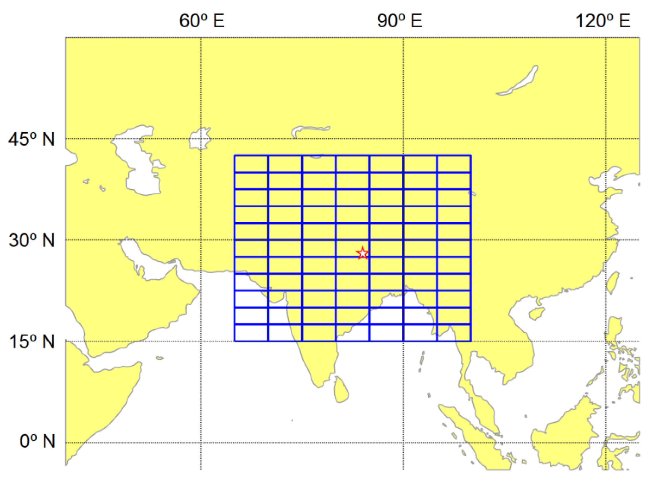
The substitution of these dm and dp by the r in Equation (1) for a particular magnitude of a subsequent earthquake (say Mw = 8) gives the possible area of disturbance in the ionosphere to be looked for in the prior GIM files, Figure 2. That is, for Mw = 8 in Equation (1) the radius r results in 2981 km. According to Equation (3), with dm equal to this length of 2981 km along the meridian and Earth’s radius R of 6371 km, this supposes an increment in latitude Δφ of 0.467894833 rad or 26.8° both north and south of the potential location of the epicenter. Taking into account the 2.5-degree spacing in the latitude of the TEC values in the GIM files, this represents some 10 cells north and south of the epicenter’s latitude. Similarly, according to Equation (4), with dp equal to this length of 2981 km along the 28° N parallel and Earth’s radius R of 6371 km, this supposes an increment in longitude Δλ of 0.529923675 rad or 30.4° both east and west of the potential location of the epicenter. Taking into account the 5-degree spacing in the latitude of the TEC values in the GIM files, this represents some 5 cells east and west of the epicenter’s longitude. Please note that, for the purposes of better visualization, the cell grid size in Figure 2 has been enlarged so that it does not correspond to the set of cells of 2.5° size in the latitude and 5° size in the longitude, while the total extent of the affected area is represented fairly faithfully.
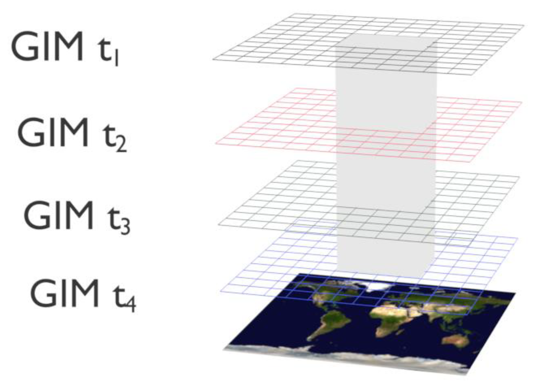
In fact, the situation is a bit more complicated: as TEC variations in both spatial and temporal components need to be analyzed, the data structures will be 3D matrices, having in the different rows and columns the TEC values for the different latitudes and longitudes, respectively, and in the third component, the different values for different times (for example every 2 h) as taken from the GIM files. This idea is depicted in Figure 3, where, instead of using a 2D matrix, a 3D matrix with the geographical area of interest for different available times in the GIMs (from the most recent one back to several days before, as seen for the purpose of prediction).

2.2. Earthquake Catalog

Now it has become clear how to retrieve the data to be analyzed in order to predict a single earthquake, I want to explain how to obtain the complete earthquake dataset that has been compiled for this study and, in the next subsection, how to work with it.
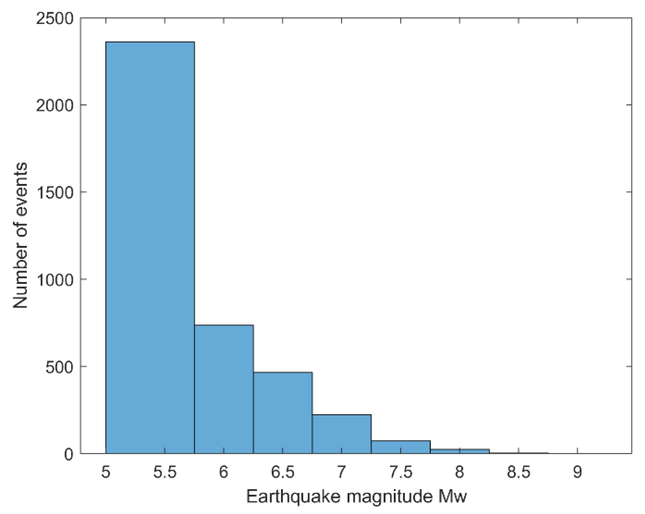
The United States Geological Survey earthquake catalog [37] was used to retrieve the set of earthquakes of magnitude Mw 5.0 or higher from 1 January 2011 to 1 October 2024, that is, almost the last 14 years. Earthquakes of magnitudes around Mw 5.5 or lower (with those below Mw 5.0 simply excluded from this study) are understood to be little significant for the prediction. To overcome a part of the overwhelming dominance of these lower-magnitude events—which could hamper the estimation capabilities of the events with the largest magnitudes—as well as to alleviate the computational requirements where possible, I have simplified the list of earthquakes to deal with by randomly selecting only 10% of the events with magnitudes below or equal to Mw 5.5; 15% of the events with magnitudes from Mw 5.6 to Mw 6.0; 50% of the events with magnitudes from Mw 6.1 to Mw 6.5; and all the events with magnitudes higher than Mw 6.5. After this operative simplification, the list of earthquakes used for training the network displays a magnitude distribution, as shown in Table 1 and Figure 4.
The earthquakes in the first group are essentially understood as having little significance for prediction purposes, so they are considered “non-significant earthquakes” for the scope of this study. Instead, this study aims to explore the largest magnitudes, with those in the groups of 7.0 and above as the main targets.

2.3. Training and Validation Data

The largest earthquake in the period of this study is the Mw 9.1 Japan earthquake that occurred on 11 March 2011, UTC 5:46, with an epicenter of latitude 38.297° N and longitude 142.373° E. This magnitude of Mw 9.1 is set to define the extent of the geographic area to search for anomalies during the whole study; that is, according to Equation (1), an abnormal area with a radius r of 8103 km is conservatively used to define the increments in latitude Δφ and longitude Δλ from the epicenter by means of Equations (3) and (4), after equating the distances along the meridian dm and the parallel dp to this radius r, to define an area of influence (refer to Figure 2, but in this case, a larger extension).
Now the idea is to go one by one through the whole earthquake list compiled previously (refer to Table 1 and Figure 4) and, for each earthquake, to construct the following:
  • A predictor variable, denoted as the X variable, from the use of the GIM files of the previous few days (excluding the file of the day of the earthquake)—that is, from 7 days before to 1 day before to predict the maximum earthquake. This X variable turns out to be a 3D matrix with the following features:
    -
    60 rows, corresponding to the latitude range explained before;
    -
    73 columns. Since the length of the parallel arc depends on its latitude different numbers of columns were obtained for the different latitudes, with high latitudes needing the whole column range in the GIM, 73. Completing with zeros the other column ranges was necessary to have a consistent size;
    -
    84 values in the third dimension, corresponding to the 7 days with data every 2 h in the GIM files;
  • A predicted variable, denoted as the Y variable, which is obtained from the earthquake list as the highest magnitude of the earthquake occurring in the area from 7 days before to 4 days after the earthquake under analysis. This is because there could be aftershocks even larger than the selected earthquake, or previous events of greater magnitude, and the predictor should capture them. The earthquake magnitude is categorized in one of eight categories named as group number in Table 1 and this category is stored as the Y variable.
It is worth mentioning that some earthquakes in the list could not be analyzed due to the lack of GIMs for those days (data gaps already mentioned in Section 2.1) leaving the total list of events to be predicted with available GIMs at 3815.
From the whole set of (X, Y) variables, 80% and 20% were selected as training and validation sets, respectively.

2.4. Convolutional Neural Networks

As previously mentioned, Convolutional Neural Networks have demonstrated a high performance in image classification. The current problem of forecasting the magnitude of future earthquakes from a number of GIMs (refer to Figure 3, which shows the data used for the prediction) can also be understood as a problem of image classification (into the categories of Table 1) from a number of GIMs that are the analog of the 3-channel RGB images.
In a previous work [26], the author presented an estimator with significant success for large earthquake prediction after the extensive testing of all earthquakes of magnitudes Mw of 4.0 or higher that occurred worldwide during the years 2011 to 2018 in the form of a nonlinear regression model. Unfortunately, the application to subsequent years has proved to be quite disappointing. Whatever the reason for this limitation, it is clear that some data typically change or evolve, as is the case for TEC values, which are certainly higher these days than between 2011 and 2018 (due to the solar cycle), and any approach, whatever it is, must evolve over time and allow for the incorporation of recent data and not remain frozen in the past.
This is why, with the solution presented here—which has been trained with data from 1 January 2011 to 1 October 2024—it is understood that it should be trained periodically with updated data.
We use a network of four convolutional layers, the first with 16, the second with 32, the third with 64, and the fourth with 128 feature maps, all of them with filters of sizes 5 × 5 and zero padding equal to one. There is also a fully connected layer which is connected to a softmax output layer, Figure 5. The Stochastic Gradient Descent with Momentum (SGDM) is used for the adjustment. The training, validation, and testing that will be later explained were all performed using the Matlab Deep Learning Toolbox [38].
Although the solutions tested so far have by no means been exhausted, the CNN approach for regression testing was not successful, while the approach with the CNN for classification has been successful, as presented later. Many ideas to improve the network design may be possible. In the spirit of a collaborative effort of this presentation, the training and validation data (that is, both the three-dimensional matrices and the magnitudes of the subsequent earthquake magnitudes for the entire dataset) are provided in this paper along with the trained network (in Matlab format) for other researchers to try to improve the design of the network to enhance the prediction results that will be presented next.

3. Results and Discussion

The neural network has been trained with the training variables mentioned in Section 2.3, which are available for the readers in Supplementary Materials S1 and S2, respectively (Xtraining and Ytraining). They comprise 80% of the earthquake-related information for the period under study (from 1 January 2011 to 1 October 2024). The remaining 20% of the information has been used for validation, these are the validation variables mentioned in Section 2.3, which are available for the readers in Supplementary Materials S3 and S4, respectively (Xvalidation and Yvalidation). As acknowledged in Section 2.2, the number earthquakes of the smallest magnitudes (mainly those below Mw 6.0) have been reduced to provide a more manageable dataset; first, because their representation in the dataset is still very abundant, and second, because following the expressions in use, Equations (1)–(4), the areas affected by earthquakes of these magnitudes are comparatively much smaller than those of the largest magnitudes. Please remember, in this regard, anomalies that could be triggered by events of magnitudes below Mw 5.5 are considered in the same group as calm periods (refer to group number 1 in Table 1) since this research is mainly aimed at the potential detection of very large earthquakes.
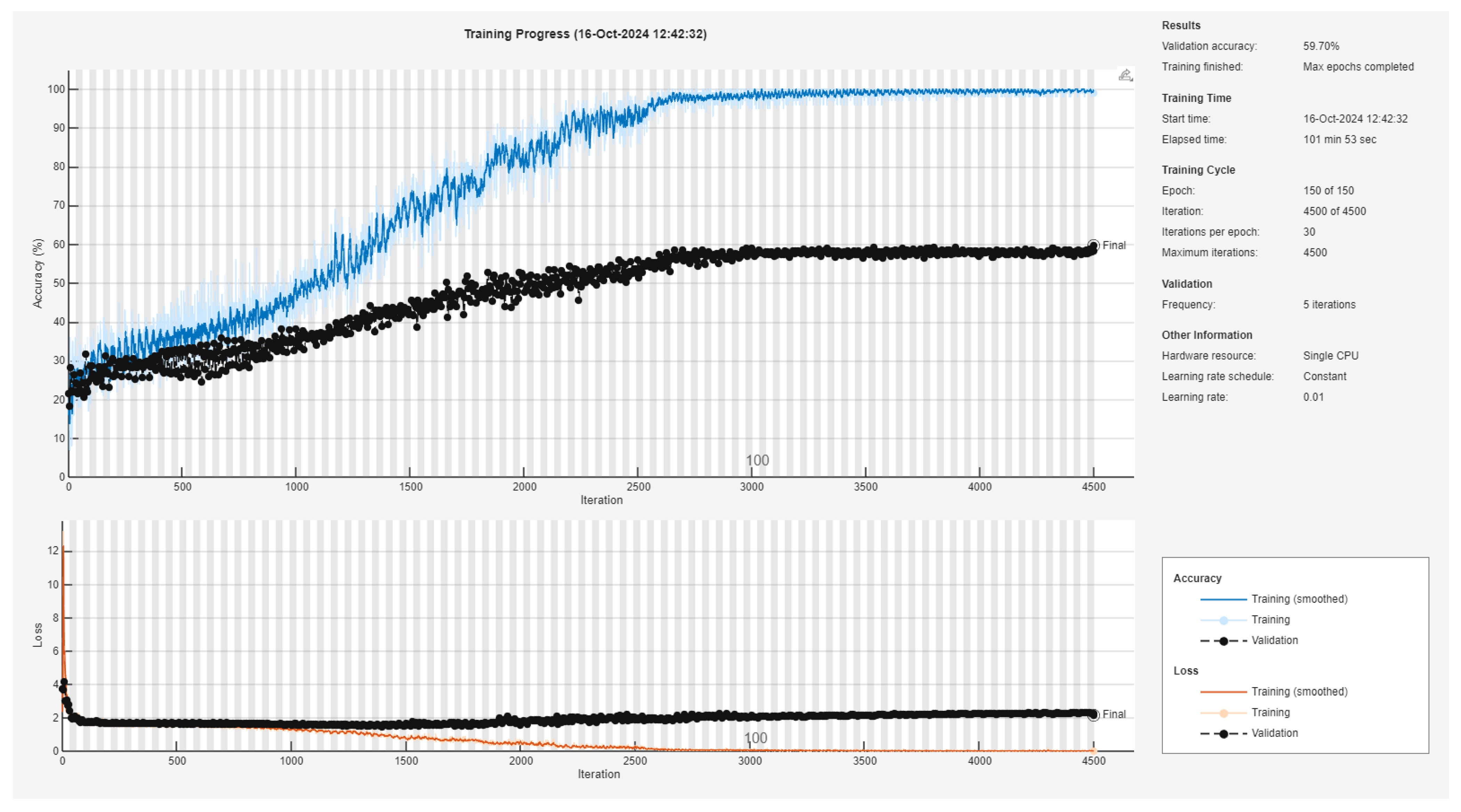
The training and validation process was performed using the Matlab Deep Learning Toolbox [38] on a standard personal computer; Figure 6 shows its evolution.
The Stochastic Gradient Descent with Momentum optimizer has been used to update the weights. It has a validation frequency of 5, which helps maintain a strong link between the validation data and training data without excessively increasing the computational burden of validation, and a minibatch size of 100, which is a value in the mid-size range commonly used for image classification. A relatively large number of epochs (150) and iterations (4500 in total, 30 per epoch) have been selected, although the accuracy of both the training and validation sets tend to stabilize a bit after reaching the middle of the calculation. Until then, a fairly gradual increase in accuracy for both the training and the validation sets is observed.
After 150 epochs, a validation accuracy of 59.70% is achieved. This is a greater success than it may seem since first, having eight categories (those in Table 1), the incorrect prediction of an earthquake with a neighboring category could also serve for the purpose of a warning system, and, second, because the magnitude values close to the interval limits (for example, a magnitude value of Mw 6.2, which belongs to category 2 but is very close to belonging to category 3, see Table 1) can be, almost equally well, attributed to both categories.
Overall, the confusion matrix obtained for the whole dataset is shown in Figure 7, where the color intensity gives an indication of the reliability according to the number of instances in each classification: in different intensities of blue for diagonal values, which refer to correct classification, and in different intensities of red for off-diagonal values, which imply misclassification and are rather pale in this case, with darker values indicating a higher number of classification errors.
As can be seen, the diagonal values clearly dominate the matrix, with adjacent categories having the second main importance. It must be considered that in the current implementation, the attributed category is the one to which the network attributes a higher probability. Other alternatives, such as performing a weighted average considering the probabilities of the different classes, could also be explored in the future.
Please remember that a single event (like the only one with a magnitude Mw above 9) can be predicted several days before (not only one day before). Figure 7 does not represent the number of earthquakes in each category but the prediction versus true numbers for the different tests.
The trained neural network is also offered to the readers in Supplementary Materials S5 in the Matlab .mat format.

4. Conclusions

Based on the proven evidence that large earthquakes are often preceded by ionospheric anomalies, the idea of an earthquake warning system based on periodically trained neural networks using GIMs has been presented. The necessary information to be collected for this purpose—three-dimensional matrices from the GIM files for the analysis of the space–time anomalies—has been introduced. The training and validation data—also using an earthquake catalog—for the whole period from 1 January 2011 to 1 October 2024 have been offered to the readers, as well as the neural network that has been trained for this purpose. The network has reached an accuracy of around 60% in the validation data for a division into eight categories of different earthquake magnitudes, a percentage that increases considerably if the classification in the neighboring categories is also accepted, something that could be clearly admissible for the purposes of a warning system.
Many ideas to enhance the network design may be possible, these are left to the reader along with the network and dataset used for the current study in order to see how much the performance can be improved, either with or without the inclusion of additional information such as, for example, indices of geomagnetic activity. The periodic updating of the network with updated GIMs, for example once a month, is in any case necessary for its application to an earthquake warning service. Although the research leading to a feasible earthquake warning system is clearly unfinished, it is firmly believed that such a system will be developed sooner or later and that one of its key components will be based, in one way or another, on a significant amount of information from the ionosphere.

Supplementary Materials

The following supporting information can be downloaded at: https://doi.org/10.5281/zenodo.14196868, Data file S1: Xtraining.mat, X variables used for training; Data file S2: Ytraining.mat, Y variables used for training; Data file S3: Xvalidation.mat, X variables used for validation; Data file S4: Yvalidation.mat, Y variables used for validation; Data file S5: net24f.mat, trained network.

Funding

This research received no external funding.

Institutional Review Board Statement

Not applicable.

Informed Consent Statement

Not applicable.

Data Availability Statement

The original contributions presented in this study are included in the Supplementary Materials, further inquiries can be directed to the author.

Conflicts of Interest

The author declares no conflicts of interest.

References

  1. Buskirk, R.E.; Frohlich, C.L.; Latham, G.V. Unusual animal behavior before earthquakes: A review of possible sensory mechanisms. Rev. Geophys. 1981, 19, 247–270. [Google Scholar] [CrossRef]
  2. Grant, R.A.; Halliday, T. Predicting the unpredictable; evidence of pre-seismic anticipatory behaviour in the common toad. J. Zool. 2010, 281, 263–271. [Google Scholar] [CrossRef]
  3. Zakharenkova, I.E.; Shagimuratov, I.I.; Krankowski, A. Features of the ionosphere behavior before the Kythira 2006 earthquake. Acta Geophys. 2007, 55, 524–534. [Google Scholar] [CrossRef]
  4. Zakharenkova, I.E.; Shagimuratov, I.I.; Krankowski, A.; Lagovsky, A.F. Precursory phenomena observed in the total electron content measurements before great Hokkaido earthquake of September 25, 2003 (M = 8.3). Stud. Geophys. Geod. 2007, 51, 267–278. [Google Scholar] [CrossRef]
  5. Liu, J.Y.; Chen, Y.I.; Chen, C.H.; Liu, C.Y.; Chen, C.Y.; Nishihashi, M.; Li, J.Z.; Xia, Y.Q.; Oyama, K.I.; Hattori, K.; et al. Seismoionospheric GPS total electron content anomalies observed before the 12 May 2008 Mw7.9 Wenchuan earthquake. J. Geophys. Res. 2009, 114, A04320. [Google Scholar] [CrossRef]
  6. Lin, J.W. Latitude-Time Total Electron Content Anomalies as Precursors to Japan’s Large Earthquakes Associated with Principal Component Analysis. Int. J. Geophys. 2011, 2011, 763527. [Google Scholar] [CrossRef]
  7. Guo, J.; Yu, H.; Li, W.; Liu, X.; Kong, Q.; Zhao, C. Total Electron Content Anomalies Before Mw 6.0+ Earthquakes in the Seismic Zone of Southwest China between 2001 and 2013. J. Test. Eval. 2017, 45, 131–139. [Google Scholar] [CrossRef]
  8. Jia, D.; Yu, H.; Zhao, B.; Ma, Y. Geothermal Anomalies and Coupling with the Ionosphere before the 2020 Jiashi Ms6.4 Earthquake. Appl. Sci. 2023, 13, 3019. [Google Scholar] [CrossRef]
  9. Pura, T.; Güneş, P.; Güneş, A.; Hameed, A.A. Earthquake Prediction for the Düzce Province in the Marmara Region Using Artificial Intelligence. Appl. Sci. 2023, 13, 8642. [Google Scholar] [CrossRef]
  10. Fuso, F.; Crocetti, L.; Ravanelli, M.; Soja, B. Machine learning-based detection of TEC signatures related to earthquakes and tsunamis: The 2015 Illapel case study. GPS Solut. 2024, 28, 106. [Google Scholar] [CrossRef]
  11. Pizza, M.; Ferrario, F.; Michetti, A.M.; Velázquez-Bucio, M.M.; Lacan, P.; Porfido, S. Intensity Prediction Equations Based on the Environmental Seismic Intensity (ESI-07) Scale: Application to Normal Fault Earthquakes. Appl. Sci. 2024, 14, 8048. [Google Scholar] [CrossRef]
  12. Huang, Y.; Zhu, P.; Li, S. Feasibility Study on Earthquake Prediction Based on Impending Geomagnetic Anomalies. Appl. Sci. 2024, 14, 263. [Google Scholar] [CrossRef]
  13. Tronin, A.A.; Hayakawa, M.; Molchanov, O.A. Thermal IR Satellite Data Application for Earthquake Research in Japan and China. J. Geodyn. 2002, 33, 519–534. [Google Scholar] [CrossRef]
  14. Pulinets, S.; Boyarchuk, K. Ionospheric Precursors of Earthquakes; Springer: Berlin, Germany, 2004; pp. 1–315. [Google Scholar]
  15. Nemec, F.; Santolík, O.; Parrot, M.; Berthelier, J.J. Spacecraft observations of electromagnetic perturbations connected with seismic activity. Geophys. Res. Lett. 2008, 35, L05109. [Google Scholar] [CrossRef]
  16. Grant, R.A.; Halliday, T.; Balderer, W.P.; Leuenberger, F.; Newcomer, M.; Cyr, G.; Freund, F.T. Ground Water Chemistry Changes before Major Earthquakes and Possible Effects on Animals. Int. J. Environ. Res. Public Health 2011, 8, 1936–1956. [Google Scholar] [CrossRef]
  17. Picozza, P.; Conti, L.; Sotgiu, A. Looking for Earthquake Precursors from Space: A Critical Review. Front. Earth Sci. 2021, 9, 676775. [Google Scholar] [CrossRef]
  18. Ouzounov, D.; Pulinets, S.; Davidenko, D.; Rozhnoi, A.; Solovieva, M.; Fedun, V.; Dwivedi, B.N.; Rybin, A.; Kafatos, M.; Taylor, P. Transient Effects in Atmosphere and Ionosphere Preceding the 2015 M7.8 and M7.3 Gorkha–Nepal Earthquakes. Front. Earth Sci. 2021, 9, 757358. [Google Scholar] [CrossRef]
  19. Freund, F. Charge generation and propagation in rocks. J. Geodyn. 2002, 33, 545–572. [Google Scholar] [CrossRef]
  20. Freund, F.T.; Takeuchi, A.; Lau, B.W. Electric currents streaming out of stressed igneous rocks—A step towards understanding pre-earthquake low frequency EM emissions. Phys. Chem. Earth 2006, 31, 389–396. [Google Scholar] [CrossRef]
  21. Freund, F.T.; Kulahci, I.G.; Cyr, G.; Ling, J.; Winnick, M.; Tregloan-Reed, J.; Freund, M.M. Air ionization at rock surfaces and pre-earthquake signals. J. Atmos. Sol. Terr. Phys. 2009, 71, 1824–1834. [Google Scholar] [CrossRef]
  22. Freund, F.T. Toward a unified solid state theory for pre-earthquake signals. Acta Geophys. 2010, 58, 719–766. [Google Scholar] [CrossRef]
  23. Warwick, J.W.; Stoker, C.; Meyer, T.R. Radio emission associated with rock fracture: Possible application to the Great Chilean Earthquake of May 22, 1960. J. Geophys. Res. Solid Earth 1982, 87, 2851–2859. [Google Scholar] [CrossRef]
  24. King, B.V.; Freund, F. Surface charges and subsurface space charge distribution in magnesium oxide containing dissolved traces of water. Phys. Rev. B 1984, 29, 5814–5824. [Google Scholar] [CrossRef]
  25. Philippetis, A.L. Electromagnetic signals before rupture and their possible interconnection with bioeffects. Modern Phys. Lett. B 2009, 23, 1431–1436. [Google Scholar] [CrossRef]
  26. Baselga, S. A combined estimator using TEC and b-value for large earthquake prediction. Acta Geod. Geophys. 2020, 55, 63–82. [Google Scholar] [CrossRef]
  27. Şentürk, E.; Çepni, M.S. A statistical analysis of seismo ionospheric TEC anomalies before 63 Mw ≥ 5.0 earthquakes in Turkey during 2003–2016. Acta Geophys. 2018, 66, 1495–1507. [Google Scholar] [CrossRef]
  28. Yao, Y.; Chen, P.; Wu, H.; Zhang, S.; Peng, W. Analysis of ionospheric anomalies before the 2011 Mw 9.0 Japan earthquake. Chin. Sci. Bull. 2012, 57, 500–510. [Google Scholar] [CrossRef]
  29. Dobrovolsky, I.R.; Zubkov, S.I.; Myachkin, V.I. Estimation of the size of earthquake preparation zones. Pure Appl. Geophys. 1979, 117, 1025–1044. [Google Scholar] [CrossRef]
  30. Hernández-Pajares, M.; Juan, J.M.; Sanz, J.; Orus, R.; Garcia-Rigo, A.; Feltens, J.; Komjathy, A.; Schaer, S.C.; Krankowski, A. The IGS VTEC maps: A reliable source of ionospheric information since 1998. J. Geod. 2009, 83, 263–275. [Google Scholar] [CrossRef]
  31. Ionosphere. International GNSS Service. Available online: https://igs.org/wg/ionosphere (accessed on 17 October 2024).
  32. Maurício, J.; Domingues, I.; Bernardino, J. Comparing Vision Transformers and Convolutional Neural Networks for Image Classification: A Literature Review. Appl. Sci. 2023, 13, 5521. [Google Scholar] [CrossRef]
  33. Pulinets, S.A.; Legen’ka, A.D.; Gaivoronskaya, T.V.; Depuev, V.K. Main phenomenological features of ionospheric precursors of strong earthquakes. J. Atmos. Sol. Terr. Phys. 2003, 65, 1337–1347. [Google Scholar] [CrossRef]
  34. Akhoondzadeh, M.; Saradjian, M.R. TEC variations analysis concerning Haiti (January 12, 2010) and Samoa (September 29, 2009) earthquakes. Adv. Space Res. 2011, 47, 94–104. [Google Scholar] [CrossRef]
  35. Gopinath, S.; Prince, P.R. Nonextensive and distance-based entropy analysis on the influence of sunspot variability in magnetospheric dynamics. Acta Geod. Geophys. 2018, 53, 639–659. [Google Scholar] [CrossRef]
  36. Paul, B.; De, B.K.; Guha, A. Latitudinal variation of F-region ionospheric response during three strongest geomagnetic storms of 2015. Acta Geod. Geophys. 2018, 53, 579–606. [Google Scholar] [CrossRef]
  37. Earthquake Catalog. U.S. Geological Survey. Available online: https://earthquake.usgs.gov/earthquakes/search/ (accessed on 17 October 2024).
  38. Deep Learning Toolbox—MATLAB—MathWorks. Available online: https://www.mathworks.com/products/deep-learning.html (accessed on 17 October 2024).
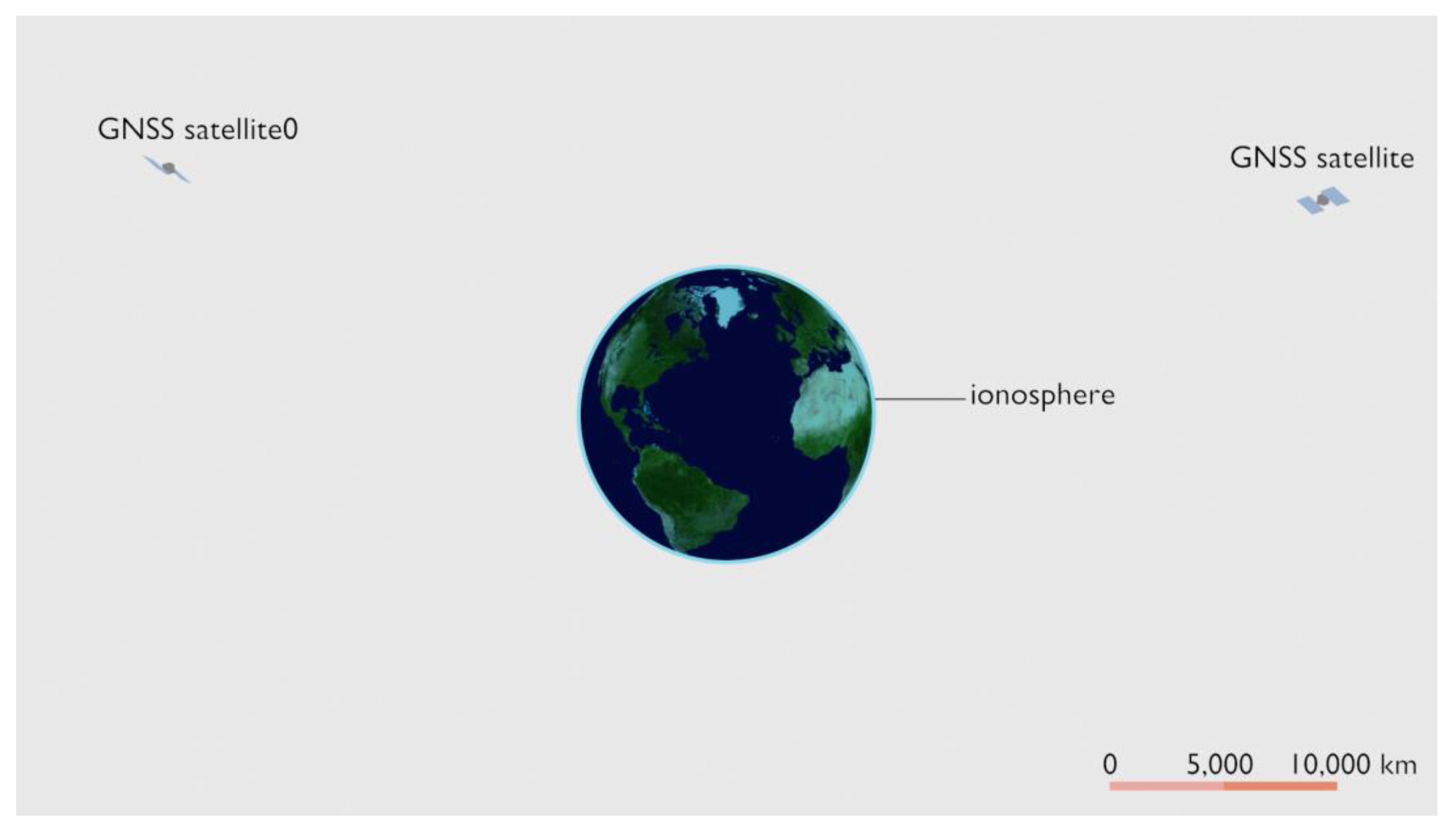
Figure 1. Earth, the ionosphere, and two example GNSS satellites at true scale (except for satellite size). It can be observed that the ionosphere compared to the total terrestrial size is as thin as the skin of an apple is compared to the whole apple, which is a reason for the strong electromagnetic coupling between the lithosphere and the ionosphere. GNSS satellites orbit the Earth at much higher altitudes but their observations at different frequencies in the L-band are sensitive to the ionosphere, since it acts as a dispersive medium.
Applsci 14 10859 g001
Figure 2. Example GIM subgrid to analyze for possible TEC anomalies. A star indicates the location of the epicenter of the earthquake of magnitude Mw = 7.8 that actually occurred on 25 April 2015.
Applsci 14 10859 g002
Figure 3. Illustration of a 3D matrix for enclosing a geographical area during several epochs t1, t2, t3, t4 included in the GIM files.
Applsci 14 10859 g003
Figure 4. Histogram of earthquake magnitudes.
Applsci 14 10859 g004
Figure 5. Scheme of the network layers.
Applsci 14 10859 g005
Figure 6. Evolution of the network training.
Applsci 14 10859 g006
Figure 7. Confusion matrix for the eight categories (here named with the central Mw values) as defined in Table 1.
Applsci 14 10859 g007
Table 1. Distribution of earthquakes under study in terms of their magnitudes.
Group NumberApproximate Magnitude MwMagnitude Mw LimitsNumber of Events
15.5 or less<5.752362
26.0[5.75, 6.25)736
36.5[6.25, 6.75)466
47.0[6.75, 7.25)224
57.5[7.25, 7.75)74
68.0[7.75, 8.25)24
78.5[8.25, 8.75)3
89.0≥8.751
Disclaimer/Publisher’s Note: The statements, opinions and data contained in all publications are solely those of the individual author(s) and contributor(s) and not of MDPI and/or the editor(s). MDPI and/or the editor(s) disclaim responsibility for any injury to people or property resulting from any ideas, methods, instructions or products referred to in the content.