Article

Accuracy of Dynamic Modulus Models of Asphalt Mixtures Containing Reclaimed Asphalt (RA)

1
Faculty of Civil Engineering, Czech Technical University in Prague, 166 29 Prague, Czech Republic
2
Polytechnic Department of Engineering and Architecture (DPIA), University of Udine, 33100 Udine, Italy
*
Authors to whom correspondence should be addressed.
Appl. Sci. 2024, 14(22), 10505; https://doi.org/10.3390/app142210505
Submission received: 7 August 2024 / Revised: 5 November 2024 / Accepted: 7 November 2024 / Published: 14 November 2024
(This article belongs to the Special Issue Rheology of Binders and Asphalt Mixtures)

Abstract

:
The dynamic modulus (∣ E * ∣) is a fundamental mechanical parameter for studying the performance of hot mix asphalt and simulating its viscoelastic behaviour under different loading and thermal conditions. It is a primary tool to replicate road surface behaviour under vehicle traffic loading and temperature variations. Though, laboratory testing to determine this parameter is time-consuming and costly. Several predictive models have been developed to estimate the dynamic modulus, ranging from rheological to empirical regression models. This research was dedicated to studying two predictive models for determining the master curve of the dynamic modulus of hot mix asphalt used in a regular pavement binder course containing different reclaimed asphalt contents (0%, 30%, 40%, and 50%). Laboratory experiments were conducted to assess their accuracy. The results show that Witczak’s sigmoid function provided the best accuracy for the master curves, while the Generalized Huet-Sayegh (2S2P1D) model showed less accurate predictions, particularly at the range of low and high frequencies.

1. Introduction

The dynamic modulus ( E * ) is a fundamental material property used to characterize the stiffness and elastic response of viscoelastic materials, such as hot mix asphalt (HMA) [1]. It is an essential parameter in the design and analysis of road pavements as it quantifies a material’s ability to resist deformation under dynamic (cyclic) loading conditions, commonly experienced by road surfaces due to vehicle traffic and temperature variations. The ∣ E * ∣ is typically determined through laboratory testing and is defined as the ratio of dynamic stress (σ) to dynamic strain (ε) experienced by a material under sinusoidal loading (see Figure 1) conditions at various temperatures [2]. Mathematically, it is represented as in Equation (1).
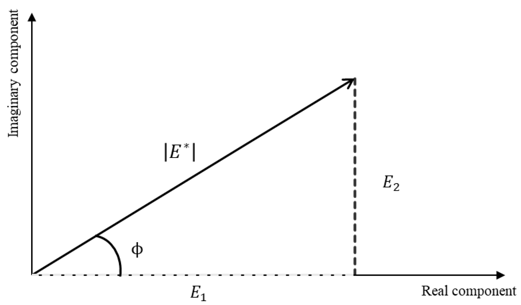
Under the noted conditions—sinusoidal loading at various temperatures—the asphalt mix behaves mainly in a linear viscoelastic manner, meaning that the material’s response to sinusoidal stress is sinusoidal, with a phase lag (Φ) between strain and stress (deformation and applied stress). Given this, the dynamic modulus ( E * ) is calculated. E * has a real part ( E 1 ) and an imaginary part ( E 2 ), as shown in Figure 2, providing essential information about the elastic, viscous, and linear viscoelastic behaviour of an asphalt mixture over a wide range of temperatures and loading frequencies.
Various test methods exist to proceed with the calculation of this modulus, with loading type varying depending on the specific test protocol. The load can be applied either in compression (axial loading) in the case of an indirect tension dynamic test or in bending in the case of 2- and 4-point bending tests. In this research, the 4-point bending test (according to EN 12697-26 Annex B) was performed, the dynamic modulus was calculated, and the master curve was then generated [3]. However, dynamic tests, including the 4-point bending test, are known to be lengthy and costly. Therefore, many researchers have explored methods for predicting the modulus, with a view to obtaining an order of magnitude that can be used in pavement design [4,5,6,7,8]. Investigations have established that there are three main methods of prediction: empirical prediction equations (based on regression analyses), meso-mechanical prediction methods (based on composite material theory), and numerical simulation (based on computer technology) [9].
In the past few years, research focusing on predicting the dynamic modulus of asphalt mixtures containing RA has increased significantly. These studies utilize various techniques, such as empirical, mechanistic, and machine learning-based, as well as hybrid models, to improve the accuracy of predictions of RA-based asphalt mixtures. To name a few, Wu et al. [9] presented an n-layer-inclusions meso-mechanical model to predict the E * of reclaimed asphalt materials. They recommended dividing asphalt layers into N = 50 layers for better prediction since the growth rate of reclaimed asphalt (predicted E * ) decreased significantly and became closer and closer after N = 50. Hossain et al. [10] evaluated the viscoelastic properties of RA-blended asphalt binders and studied the Witczak model’s ability to estimate the dynamic modulus master curves of asphalt mixtures containing reclaimed asphalt. They concluded that the Witczak model is capable of predicting E master curves of these types of mixtures. Finally, Dao et al. [11] used various machine learning-based algorithms such as support vector machines (SVMs), artificial neural networks (ANNs), ensemble boosted trees (Boosted), and Gaussian process regression (GPR) to predict the dynamic modulus of warm mix asphalt with different contents of reclaimed asphalt. They found that the Boosted algorithm provided the best simulation of E * compared to the other above-mentioned algorithms.
The Witczak statistical model [5] and the Hirsch model [12] were among the first models used to evaluate the dynamic modulus and phase shift angle at specific temperatures and stresses, taking into account the characteristics of the mix.
The Witczak 1-37A [13] and Witczak 1-40D [5] models are the most popular models for predicting the dynamic modulus of a conventional virgin asphalt mixture. These two empirical regression models are based on a sigmoidal function. The good prediction ability of these methods has led to their incorporation into the Mechanistic–Empirical Pavement Design Guide (MEPDG) for pavement design.
E * = σ ε
where σ represents the dynamic stress applied to the material and ε represents the dynamic strain or deformation of the material.
Maxwell, Kelvin–Voigt, Di Benedetto–Neifer (2S2P1D), Huet–Sayegh, and Prony series present the linear viscoelastic behaviour of bituminous materials and model the dynamic modulus as a composition of springs and the elastic elements and linear dampers as the Newtonian viscous elements.
All the aforementioned models proved to have some limitations depending on the mixture properties and temperature level (especially at high and low temperatures). In this context, it is necessary to study the accuracy of some of these predictive models on different asphalt mixtures [14,15,16].
This research was therefore dedicated to studying the accuracy of some of the predictive models: Witczak and generalized Huet–Sayegh models to predict the master curve on asphalt mixtures (asphalt concrete—AC) containing different contents of reclaimed asphalt.

2. Theoretical Background: Predictive Models

2.1. Witczak Model: Sigmoid Function

Research conducted at the University of Maryland [17] demonstrated that the master curve of asphalt can be represented by a sigmoid function. This method, established by Pellinen and Witczak [17], involves constructing the master curve by adjusting the parameters of the sigmoid function based on laboratory measurements of the dynamic modulus measured using a nonlinear regression method.
L o g E * = δ + α 1 + e β γ L o g f r ,
E * is the dynamic modulus (MPa); α ,   β ,   γ , and δ are the regression parameters; and f r is the reduced frequency (Hz) defined by the following relation.
f r = a T × f L o g f r = L o g a T + L o g f ,
a T is the shift factor, f is the tested frequency at the temperature T (Hz), and T is the tested temperature (°C).
This sigmoid model varies between L o g E * m i n   δ and L o g E * m a x   δ + α of the mix, based on two shape parameters ( β   ,   γ ), depending on the reduced frequency f r , as determined according to the principle of time–temperature superposition. In this equation, the parameter γ influences the slope of the function (the rate of variation between the maximum and the minimum), while the parameter β influences the horizontal position of the point of rotation (Figure 3). In addition, the coefficients α and δ depend on the particle size composition of the mixture, the asphalt binder content, and the air void content. The coefficients β and γ depend on the properties of the binder and the magnitude of δ and α . The determination of these parameters is simply performed using the SOLVER function of Microsoft Excel 2016, which involves varying the parameter values in order to fit the measured data.
Many methods existing in the literature help define the shift factor, such as the Williams–Landel–Ferry (WLF) equation, the Arrhenius equation, Generalized Time–Temperature Superposition (GTTS), and empirical or semi-empirical methods. In the case of this study, graphic determination was used. The isotherms were translated horizontally until they fit an adjacent isotherm relative to a fixed temperature (in this study, the reference temperature was set to 20 °C), based on the principle of time–temperature superposition. With this method, the translation factors were dependent on the adjustment criteria.

2.2. Generalized Huet–Sayegh Model (2S2P1D)

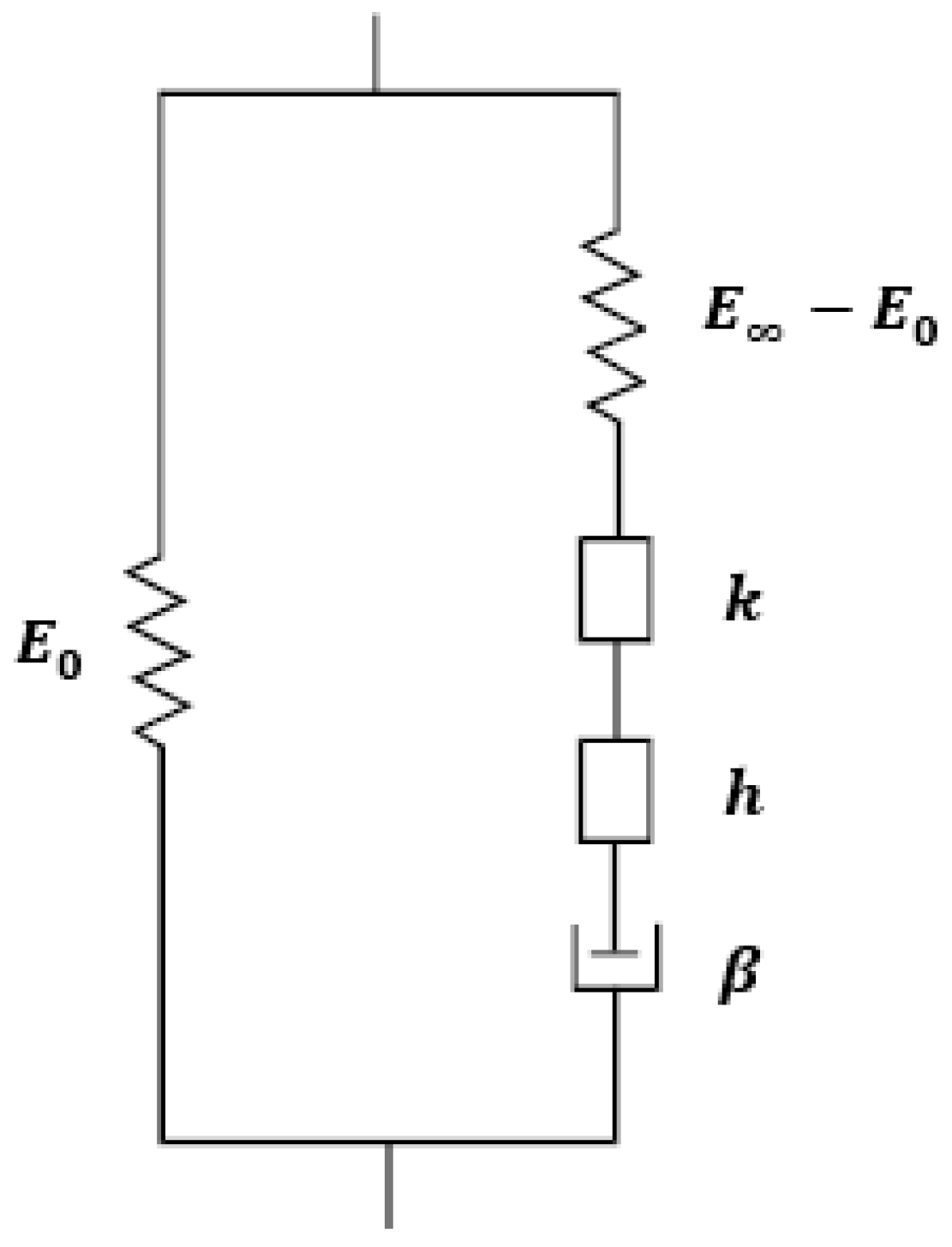
The 2S2P1D model consists of two springs, two parabolic elements, and one dashpot, hence the name. It is an adaptation of the Huet–Sayegh model, with an additional linear dashpot placed in a series with the parabolic elements and the spring of rigidity (see Figure 4). This model is suitable for characterizing the viscoelastic properties of asphalt mixtures and asphalt binders, which exhibit both elastic and viscous responses under dynamic loading [19]. This simplified model can be used for analysis and design purposes in pavement engineering to predict a material’s behaviour under various loading conditions.
The dynamic module of the Generalized Huet–Sayegh model is given by the following expression:
E * i ω = E 0 + E E 0 1 + α   ( i ω τ ) k + ( i ω τ ) h + ( i ω τ β ) 1 ,
The model consists of nine parameters, from which six are expressed explicitly in the previous equation: E 0 is the high-temperature stiffness; E is the purely elastic modulus; α ,   k ,   a n d   h are characteristics of the parabolic elements and set as 0 < k < h < 1 ; and β is the Newtonian viscosity of the dashpot. As for the other three parameters, they are determined implicitly using τ , the time characteristic, and calculated as follows.
L n τ = a + b T + c T ² ,
a ,   b , and c are regression constants representing the material characteristics.
The parameters of the 2S2P1D model were fitted by non-linear regression and successive approximations until a good visual fit was obtained between the curve given by the models and the experimental results. The method for determining these parameters involved minimizing the sum of the distances between the experimental dynamic modulus and that of the model, introduced at N points of pulsation ωi (Least Square Method). This minimisation was performed at the reference temperature TR = 20 °C using the MS Excel SOLVER function as follows:
M i n   i = 1 N ( E 1 e x p ω i E 1 m o d e l ω i 2 + E 2 e x p ω i E 2 m o d e l ω i 2 ,
E 1 e x p   and E 2 e x p   are, respectively, the real and imaginary parts of the experimental dynamic modulus E * e x p . E 1 m o d e l   and E 2 m o d e l   are, respectively, the real and imaginary parts of the dynamic modulus E * m o d e l given by the Generalized Huet–Sayegh model.

3. Experimental Materials and Testing

In this study, dynamic modulus tests were conducted on four asphalt mixtures with varying RA contents (0%, 30%, 40%, and 50%). The test data were used to determine the parameters of both models—sigmoid and Generalized Huet–Sayegh (2S2P1D)—and the accuracy of these models was evaluated.
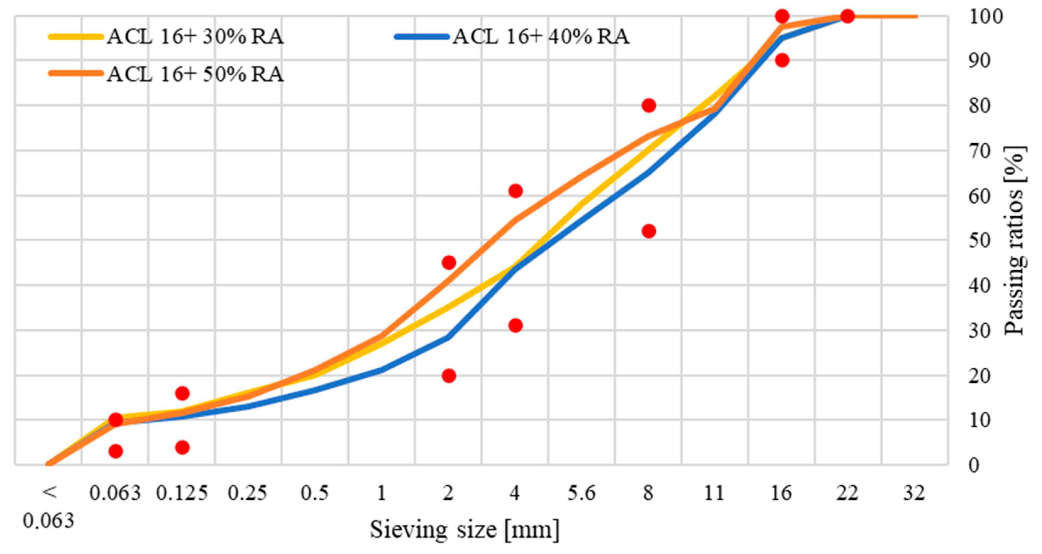
The used asphalt mixtures were graded with a nominal maximum aggregate size of 16 mm, as shown in Figure 5, and were described as shown in Table 1. All mixtures had a targeted binder content of 4.5% by weight, distributed between binder reactivated from reclaimed asphalt and added virgin binder. The added asphalt binder was 50/70 paving-grade asphalt binder, which is the most commonly used asphalt binder in the Czech Republic (see Table 2).
Table 1. Basic used mixture’s characteristics.
0%30%40%50%EN Standard
Bulk density [g.cm−3]2.3922.3682.4002.390EN 12697-6 [20]
Maximum density [g.cm−3]2.5382.5202.5242.553EN 12697-5 [21]
Voids content [%-vol.]5.76.04.96.4
Moisture susceptibility, ITSR [%]94.077.471.479.6EN 12697-12 [22]
Stiffness @15 °C [MPa]765410,76011,15917,497EN 12697-26, annex C [3]
Fracture toughness [N/mm3/2]35393839EN 12697-44 [23]
Added virgin asphalt binder [% mass]02.72.01.6
Total asphalt binders in the mix [% mass]4.54.54.54.5
Table 2. Asphalt binder 50/70 properties.
50/70 Asphalt Binder PropertiesEN Standard
Penetration @25 °C [0.1 mm]54EN 1426 [24]
Softening point (R&B) [°C]50EN 1427 [25]
Figure 5. Aggregate gradation of the asphalt mixture (red dots represent ACL aggregate gradation limits according to ČSN 73 6121:2019 [26].
Applsci 14 10505 g005
The reclaimed asphalt was collected from a cooperating asphalt mixing plant and its grading was characterized according to EN 13 108-1 [27] and CSN 73 6121 [26] standards (see Table 3). RA was then fractionated and stored in the laboratory in two fractions: fine/medium fraction (0/8 mm) and coarse fraction (8/16 mm) and characterized as follows:
A steel segment roller was used to compact a slab measuring 405 mm in length, 300 mm in width, and 50 mm, in accordance with EN 12697-33 [28]. This slab was then cut into 5 prismatic samples, each measuring 405 mm in length, 50 mm in width, and 50 mm in height.
The dynamic modulus test was conducted under a controlled strain with a fixed value of 50 micro-strains according to the European Standard EN 12697-26 at four temperatures, 0 °C, 10 °C, 20 °C, and 30 °C, and at eleven selected frequencies, 50 Hz, 30 Hz, 20 Hz, 15 Hz, 10 Hz, 8 Hz, 5 Hz, 3 Hz, 2 Hz, 1 Hz, and 0.1 Hz, for each temperature, using a Cooper research technology setup. During this test, the asphalt mixture sample was fixed at two endpoints, and sinusoidal loading was applied to two central points. The required force of deformation was measured as a function of time and phase lag. The dynamic modulus was then calculated:
E * = E 1 2 + E 2 2 ,
The phase angle was calculated as follows:
Φ = tan 1 E 2 E 1 ,

4. Experimental Results: Master Curve Construction

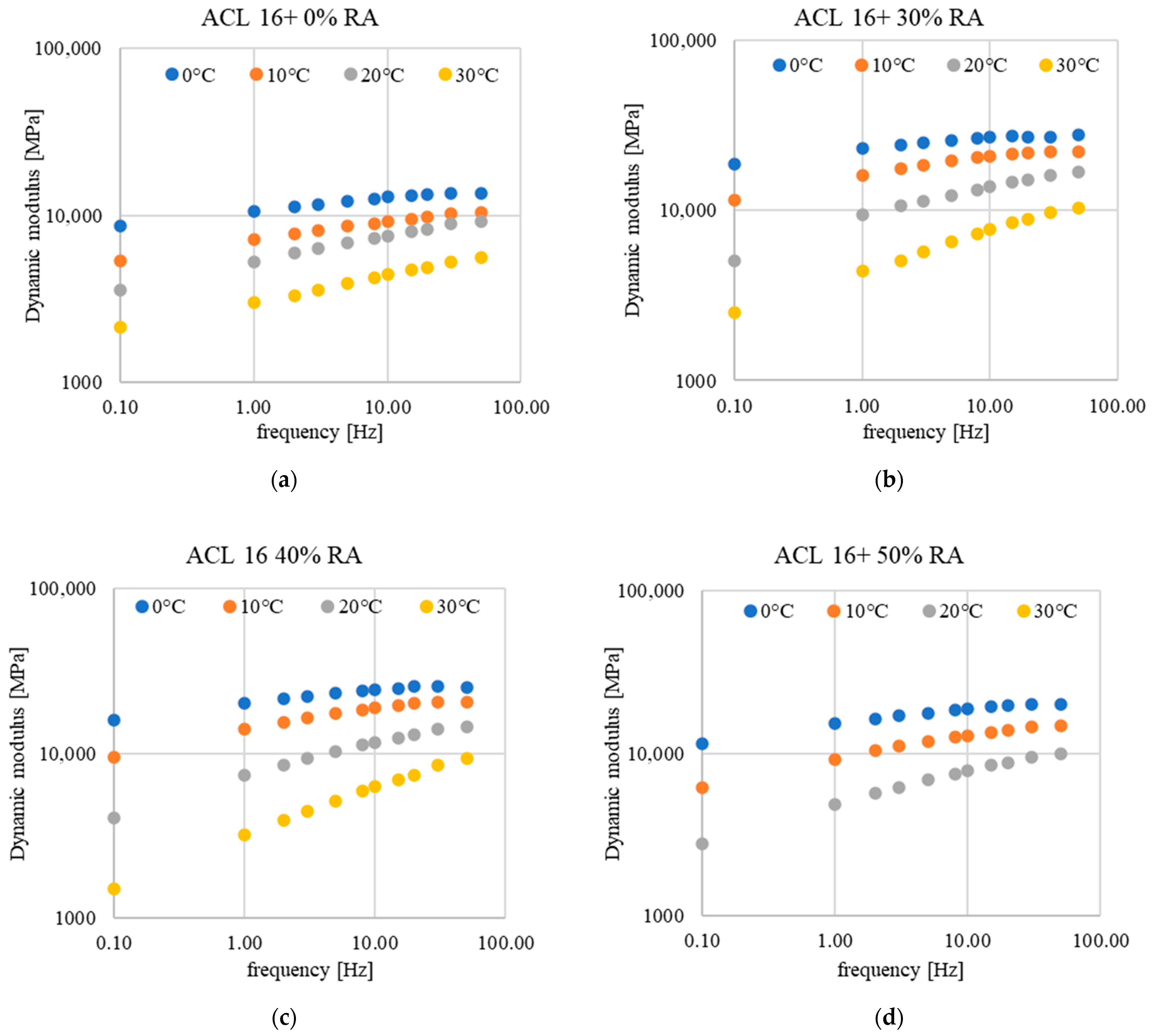
From the tested data ( E 1 and E 2 ), the dynamic modulus ( E * ) of each asphalt mixture was calculated and then plotted as a function of frequency for each temperature, T. These curves are called isothermal curves. Figure 6 shows the isothermal curves for all tested mixtures. For the mixture with 50% RA, the isothermal curve at 30 °C is missing due to inconsistencies in the dynamic values around that temperature compared to the former temperatures.
Using the principle of time–temperature superposition, the isothermal curves were shifted to create a single smooth curve, referred to as the master curve. This curve provides a clearer understanding of the deformation behaviour of asphalt mixtures across a broader range of conditions. It also establishes a relationship between the dynamic modulus and reduced frequency on a log–log scale. The reduced frequency ( ω r ) was calculated as follows:
ω r = ω × 10 log a T ,
where ω r is the reduced frequency at a defined temperature (Hz), ω is the frequency (Hz), log a T is the shift factor, and T is the Temperature (°K).
As for the shift factor, it was defined as the amount of horizontal shifting required for each isothermal curve at each temperature to be shifted following the defined temperature called the reference temperature T R . In this study, T R   = 20 °C [29]. These shifts were determined manually using Microsoft Excel, as shown in Table 4, and the master curves were plotted (see Figure 7).

5. Parameter Acquisition

5.1. Time–Temperature Superposition

In dynamic modulus prediction models, the concept of “time–temperature superposition” (referred to as “characteristic time”) is used to interpret the influence of temperature on material properties and predict their behaviour at different loading rates. This concept is important for asphalt mixtures, as they exhibit significant viscoelastic behaviour and are sensitive to temperature changes.
The characteristic time (τ) is the time scale used to shift the isothermal curves in the previous sections and generate the master curve. It is calculated as follows:
L n τ = a + b T + c T ² ,
a ,   b , and c are regression constants representing the material characteristics.
In this part, the resulting regression constants are presented for the tested asphalt mixtures in Table 5. It is shown that the values of “a” and “b” were close to each other for the different reclaimed asphalt mixtures, but the values of “c” were different.

5.2. Witczak Model: Sigmoid Function

To plot the master curve of the mixtures, the regression coefficients α, β, γ, and δ of the sigmoid function (predefined in 0) were determined using the nonlinear regression method in Microsoft Excel’s SOLVER function. These regression coefficients are presented in Table 6 for each asphalt mix tested at the same reference temperature, TR = 20 °C.
These coefficients, α, β, γ, and δ, were close for both asphalt mixtures with 0% RA and 30% RA, but they were different for the rest. The difference between these parameters could have been due to the fact that the addition of 30% RA and less has proven negligible influence on the mechanical properties of asphalt mixtures compared to higher reclaimed asphalt content mixtures.
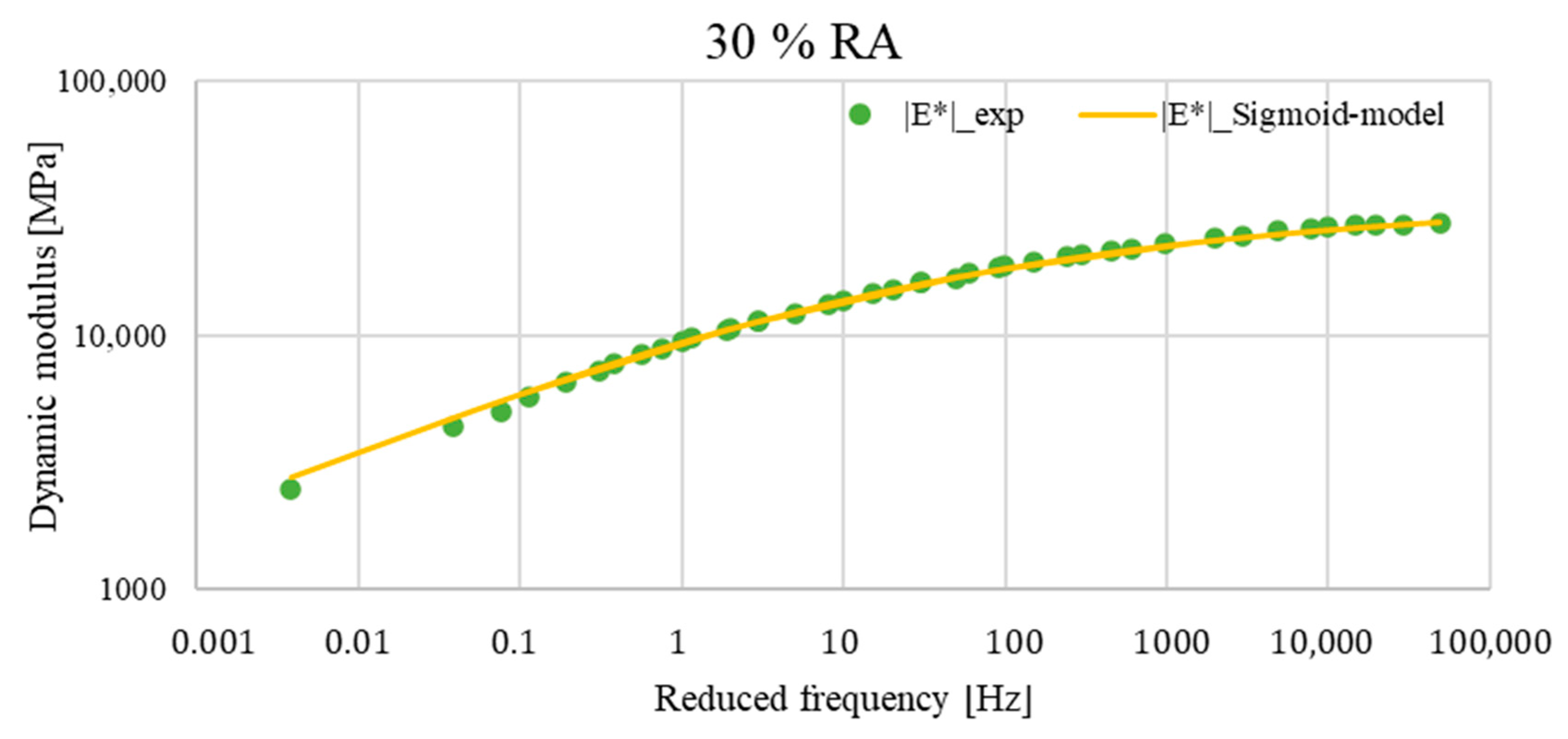
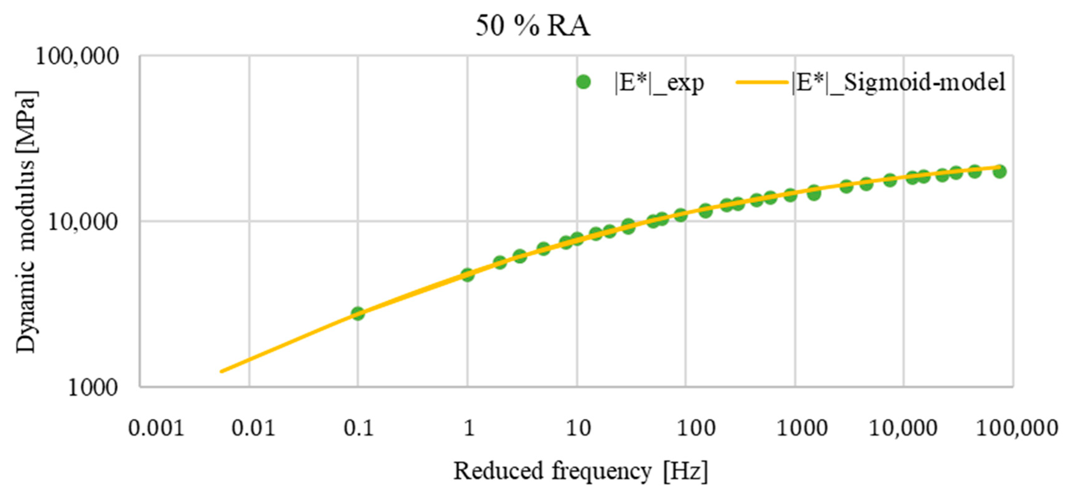
The master curves of E * for the different asphalt mixtures tested are presented as a function of reduced frequency at the reference temperature of 20 °C in Figure 8, Figure 9, Figure 10 and Figure 11.
The evaluation of the master curves showed that the dynamic modulus estimated by the sigmoid function was almost identical to the actual measurement of the dynamic modulus determined in the laboratory. The worst fit was observed for the mixture with 0% reclaimed asphalt content, where the sigmoid model overestimated the dynamic modulus values across the entire range of frequencies and, thus, temperatures. Nevertheless, the sigmoidal model effectively captured the viscoelastic behaviour.
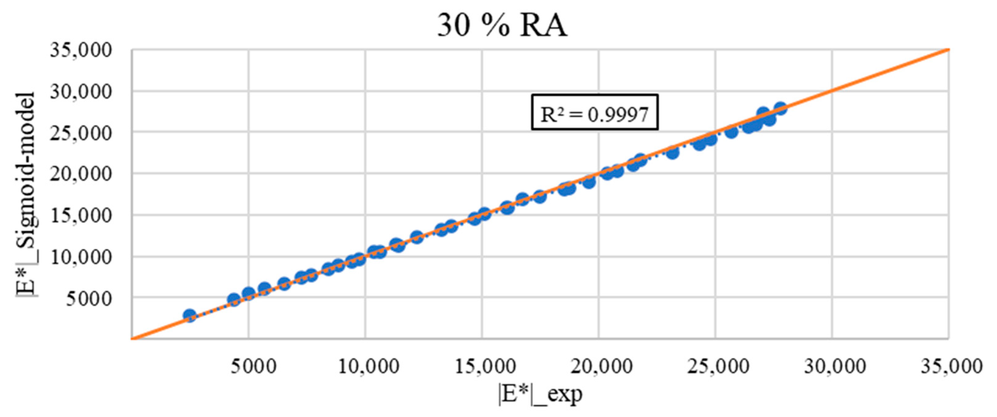
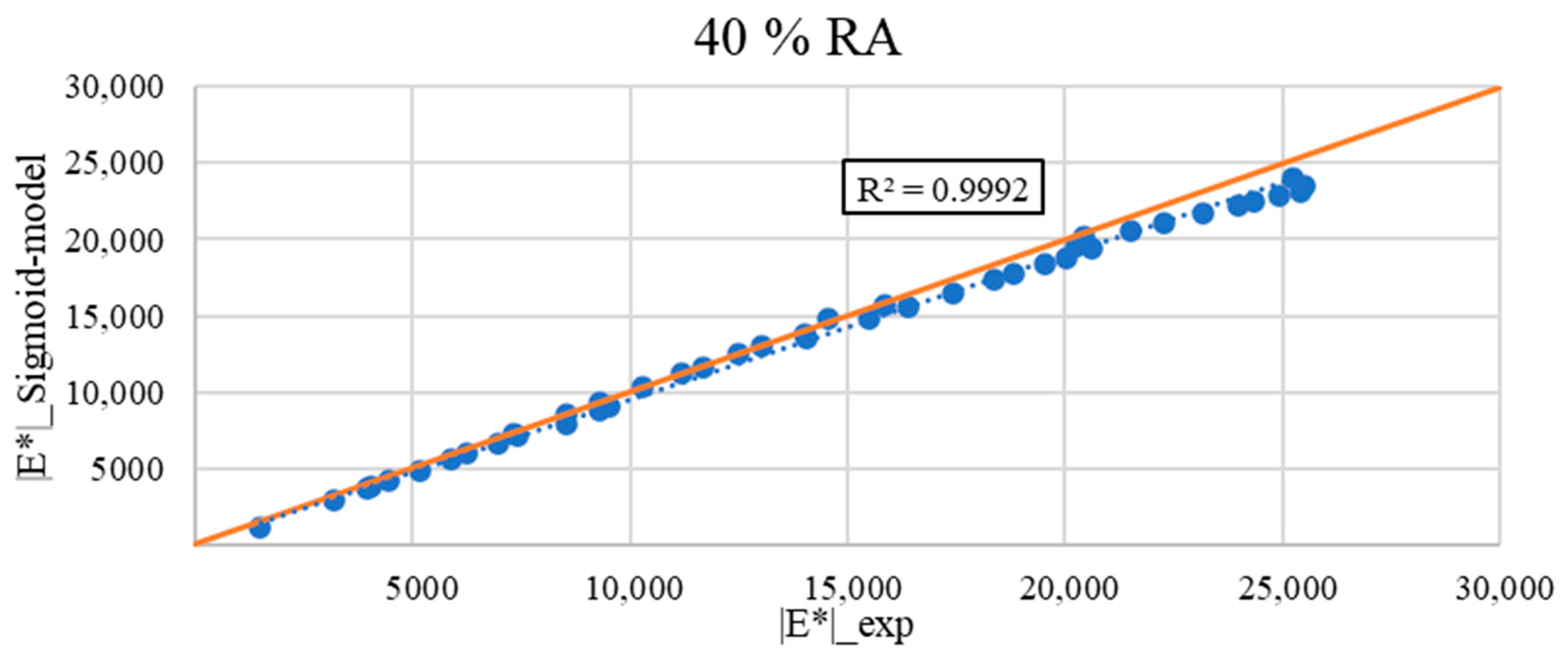
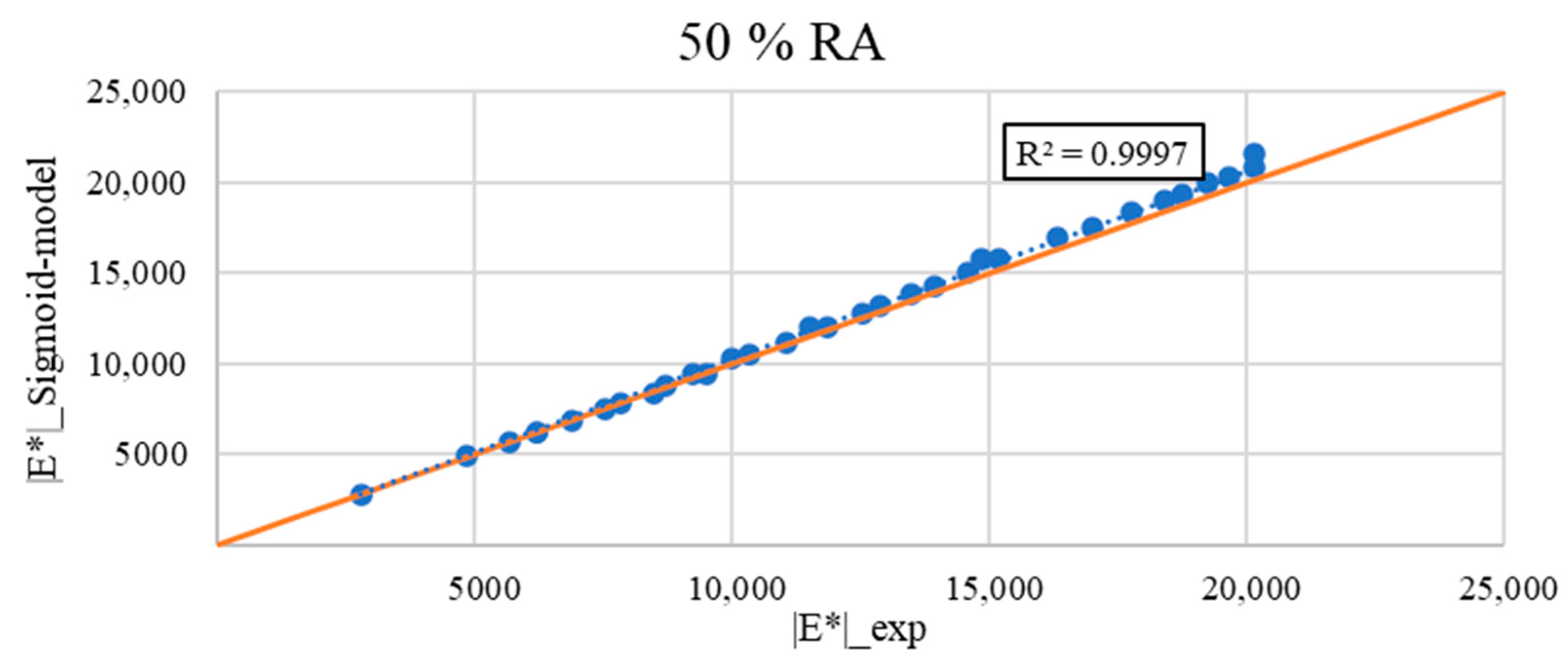
Figure 12, Figure 13, Figure 14 and Figure 15 show the calculated E *   as a function of the measured E * of all the asphalt mixes tested. The figures demonstrate good accuracy and correlations between the measured and calculated dynamic moduli for all the tested mixtures, except for the virgin mixture. Yet, the coefficient of determination (R2) for all the mixtures was around 0.99. For all the asphalt mixes, it can be observed that the points are almost perfectly aligned along a straight line where y = x.

5.3. Generalized Huet–Sayegh Model (2S2P1D)

For the second model, the 2S2P1D model, the regression coefficients α, β, k, and h were determined to plot the master curve of the mixtures. These coefficients, predefined as 0, were obtained using the nonlinear regression method with the SOLVER function in Microsoft Excel. The coefficients for each asphalt mix are provided in Table 7, with the same reference temperature, TR = 20 °C.
The k parameter affected the left asymmetry of the Cole–Cole curve and the height of the Black space curve, while the h parameter affected the radius of the Black space and Cole–Cole curves. The α parameter affected the height of the Cole–Cole curve and the right asymmetry of the Black curve, and the β typically represented the distribution of relaxation times in the material, describing the overall shape of the relaxation spectrum.
Additionally, the Cole–Cole diagram and Black space diagram helped to obtain the dynamic modulus limits, i.e., E0 and Einf. The Black space diagram is the result of plotting the dynamic modulus |E*| versus the phase angle Φ (Figure 16a). The Cole–Cole diagram (Figure 16b) illustrates the storage modulus E1 and the loss modulus E2. These two diagrams are considered valuable tools since they evaluate the materials independently of the time–temperature superposition principle.
It is evident that all the mixtures shared almost the same value for the parameter β. It is also clear that the model parameters for the mixtures with 30% RA and 40% RA were close to each other, which could have been due to the slight difference in the reclaimed asphalt compared to the other mixtures.
The E *   master curves for the tested asphalt mixes are presented as a function of frequency for the reference temperature of 20 °C in Figure 17, Figure 18, Figure 19 and Figure 20.
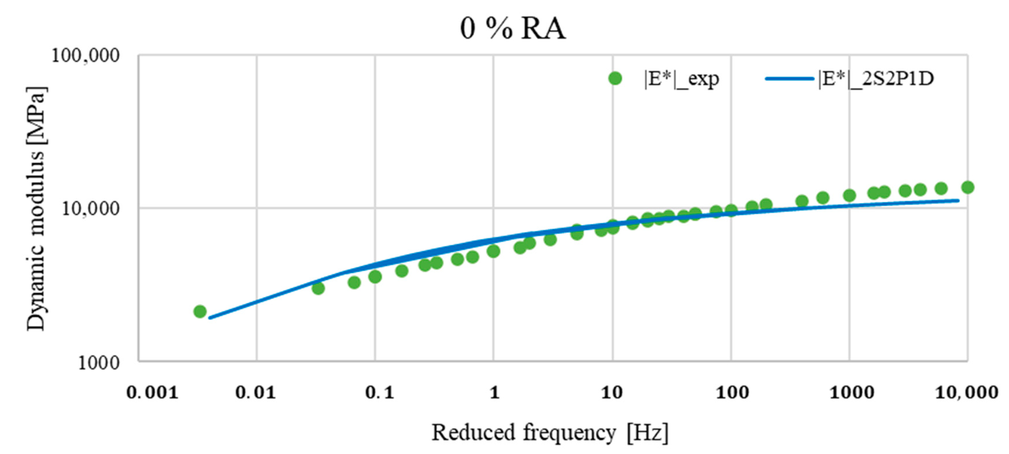
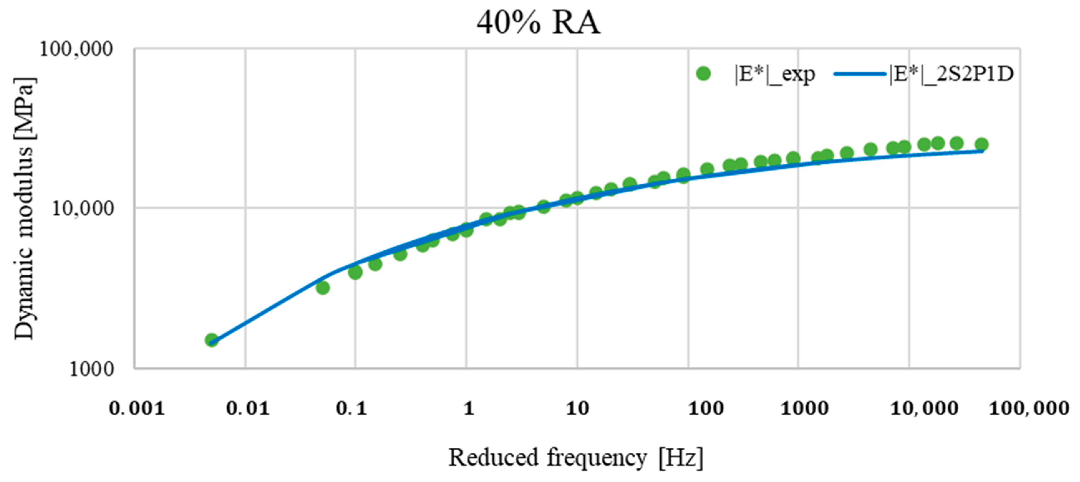
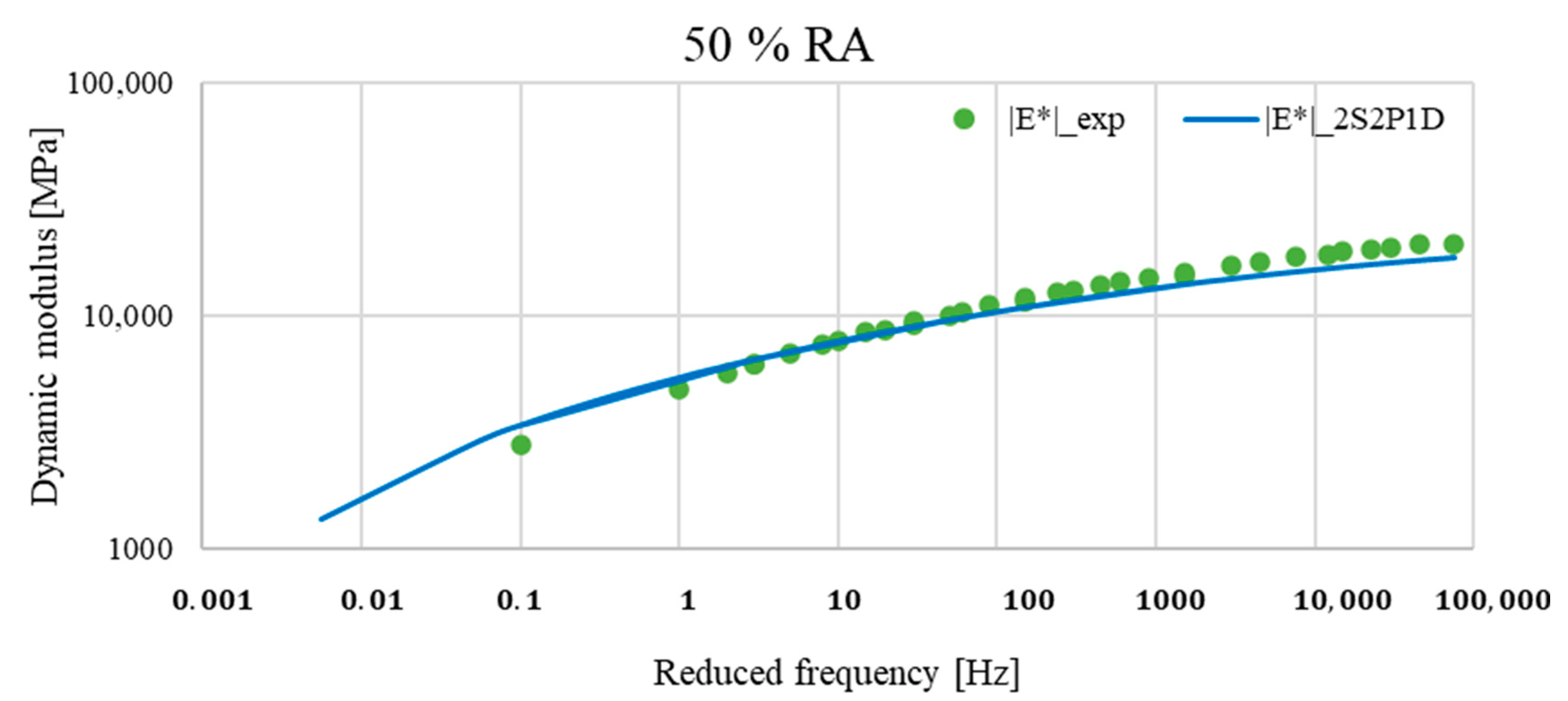
The evaluation of the master curves showed that the dynamic modulus estimated by the Generalized Huet–Sayegh model differed from the actual laboratory measurements, particularly in the range of low and high frequencies. However, these differences varied from one mixture to another.
This suggests that the 2S2P1D model did not represent the linear behaviour of asphalt mixes at low and high frequencies, and modifications to the model are required.
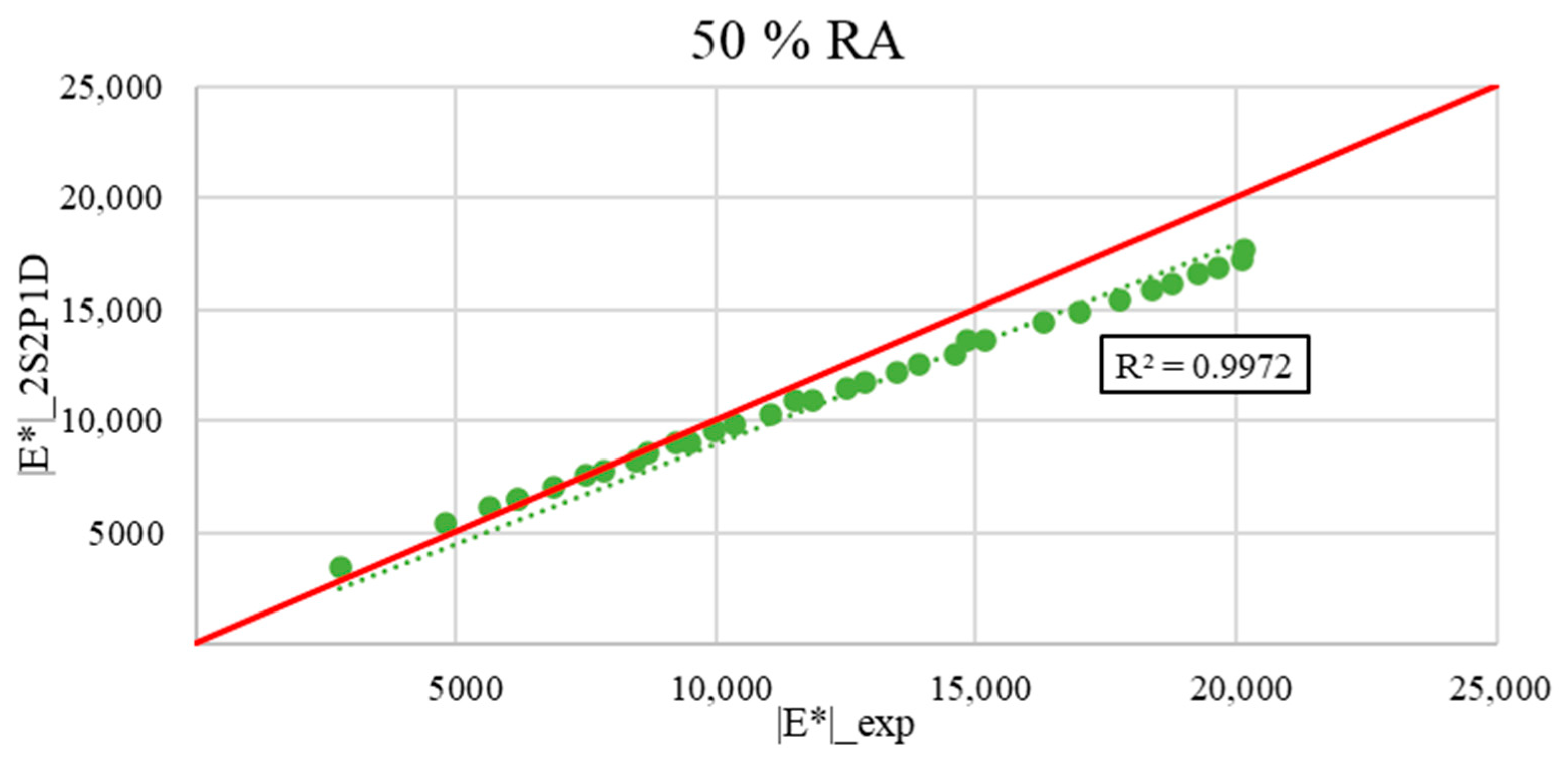
Figure 21, Figure 22, Figure 23 and Figure 24 show the calculated E * as a function of the measured E * for all the asphalt mixes tested.
The figures demonstrate good accuracy and correlations between the experimental dynamic moduli and those estimated by the Generalized Huet–Sayegh model at low frequencies. At the range of the high frequencies, the data fall below the line of the identity function. Yet, the difference is not too high.

6. Conclusions

This study examined the accuracy of two different types of dynamic modulus master curve prediction models: the sigmoid function proposed by the Witczak model and the Generalized Huet–Sayegh model, also known as the 2S2P1D model. These models were applied to four asphalt mixtures with identical aggregate types but varying reclaimed asphalt contents (0% RA, 30% RA, 40% RA, and 50% RA), all of the same gradation and binder content.
It was proven that the sigmoid function is the most effective for characterizing the master curves of reclaimed mixtures. The comparison of the measured modulus vs. the calculated modulus along the identity function confirmed this conclusion. All the tested data achieved R² values close to 1, with almost perfect alignment along the line of best fit.
On the other hand, the 2S2P1D model showed a less accurate prediction of the dynamic master curves, especially at low and high frequencies. In these ranges, the model tended to underestimate the dynamic modulus of the reclaimed mixtures. Nevertheless, the overall fitting was quite good. Further optimization of the model is required.

Author Contributions

Conceptualization, M.B. and J.V.; methodology, M.B. and J.V.; investigation, M.B.; resources, J.V. and N.B.; data curation, M.B.; writing—original draft preparation, M.B.; writing—review and editing, J.V. and N.B.; visualization, M.B., J.V. and N.B.; supervision, J.V. and N.B.; project administration, J.V. and N.B. All authors have read and agreed to the published version of the manuscript.

Funding

This study was conceptualized and developed as part of activities related to the project GA22-04047K funded by the Czech Scientific Foundation (GACR).

Institutional Review Board Statement

Not applicable.

Informed Consent Statement

Not applicable.

Data Availability Statement

The data that support the findings of this study are available from the corresponding author upon reasonable request.

Conflicts of Interest

The authors declare no conflicts of interest.

References

  1. Pellinen, T.K. Investigation of the Use of Dynamic Modulus as an Indicator of Hot Mix Asphalt; Arizona State University: Tempe, AZ, USA, 2001. [Google Scholar]
  2. Witzcak, M.W. Simple Performance Test for Superpave Mix Design; Transportation Research Board: Washington, DC, USA, 2002; Volume 465. [Google Scholar]
  3. EN 12697-26; Bituminous Mixtures—Test Methods for Hot Mix Asphalt—Part 26: Stiffness. European Committee for Standardization: Brussels, Belgium, 2012.
  4. Witczak, M.W.; Bari, J. Development of a Master Curve (E*) Database for Lime Modified Asphaltic Mixtures; Arizona State University Research Report; Arizona State University: Tempe, AZ, USA, 2004. [Google Scholar]
  5. Bari, J. Development of a New Revised Version of the Witczak E* Predictive Models for Hot Mix Asphalt Mixtures. Ph.D. Dissertation, Arizona State University, Tempe, AZ, USA, 2005. [Google Scholar]
  6. Shu, X.; Huang, B. Micromechanics-based dynamic modulus prediction of polymeric asphalt concrete mixtures. Compos. Part B Eng. 2008, 39, 704–713. [Google Scholar] [CrossRef]
  7. Cho, Y.H.; Park, D.W.; Hwang, S.D. A predictive equation for dynamic modulus of asphalt mixtures used in Korea. Constr. Build. Mater. 2010, 24, 513–519. [Google Scholar] [CrossRef]
  8. Zhu, H.; Sun, L.; Yang, J.; Chen, Z.; Gu, W. Developing master curves and predicting dynamic modulus of polymer-modified asphalt mixtures. J. Mater. Civ. Eng. 2011, 23, 131–137. [Google Scholar] [CrossRef]
  9. Wu, H.; Zhan, Y.; Song, W.; Xu, S.; Chen, X.; Liao, H. Prediction modelling on dynamic modulus of recycled asphalt mixtures based on meso-mechanical analysis. J. Clean. Prod. 2024, 469, 143200. [Google Scholar] [CrossRef]
  10. Hossain, Z.; Zaman, M. Prediction of Dynamic Modulus of Hot Mix Asphalts with Reclaimed Asphalt Pavement. Adv. Civ. Eng. 2020, 2020, 8672654. [Google Scholar] [CrossRef]
  11. Dao, D.V.; Nguyen, N.L.; Ly, H.B.; Pham, B.T.; Le, T.T. Cost-effective approaches based on machine learning to predict dynamic modulus of warm mix asphalt with high reclaimed asphalt pavement. Materials 2020, 13, 3272. [Google Scholar] [CrossRef] [PubMed]
  12. Al-Khateeb, G.; Shenoy, A.; Gibson, N.; Harman, T. A new simplistic model for dynamic modulus predictions of asphalt paving mixtures. Assoc. Asph. Paving Technol. 2006, 75. [Google Scholar]
  13. Witczak, M.W.; Fonseca, O.A. Revised predictive model for dynamic (complex) modulus of asphalt mixtures. Transp. Res. Rec. 1996, 1540, 15–23. [Google Scholar] [CrossRef]
  14. Far, M.S.S. Development of New Dynamic Modulus (E*) Predictive Models for Hot Mix Asphalt Mixtures; North Carolina State University ProQuest Dissertations Publishing: Raleigh, NC, USA, 2011. [Google Scholar]
  15. Schwartz, C.W. Evaluation of the Witczak dynamic modulus prediction model. In Proceedings of the 84th Annual Meeting of the Transportation Research Board, Washington, DC, USA, 9–13 January 2005. [Google Scholar]
  16. Ceylan, H.; Schwartz, C.W.; Kim, S.; Gopalakrishnan, K. Accuracy of predictive models for dynamic modulus of hot-mix asphalt. J. Mater. Civ. Eng. 2009, 21, 286–293. [Google Scholar] [CrossRef]
  17. Garcia, G.; Thompson, M. HMA Dynamic Modulus Predictive Models (A Review); FHWA-ICT-07-005; Illinois Center for Transportation: Rantoul, IL, USA, 2007. [Google Scholar]
  18. Tóth, C.; Ureczky, J. Determination of master curves for asphalt mixtures by means of IT-CY tests. Period. Polytech. Civ. Eng. 2010, 54, 137–142. [Google Scholar] [CrossRef]
  19. Benedetto, H.D. Modelling the rheological properties of bituminous binders using the 2S2P1D Model. Constr. Build. Mater. 2013, 38, 395–406. [Google Scholar]
  20. EN 12697-6; Bituminous Mixtures—Test Methods—Part 6: Determination of Bulk Density of Bituminous Specimens. European Committee for Standardization: Brussels, Belgium, 2018.
  21. EN 12697-5; Bituminous Mixtures—Test Methods—Part 5: Determination of the Maximum Density. European Committee for Standardization: Brussels, Belgium, 2018.
  22. EN 12697-12; Bituminous Mixtures—Test Methods—Part 12: Determination of the Water Sensitivity of Bituminous Specimens. European Committee for Standardization: Brussels, Belgium, 2018.
  23. EN 12697-44; Bituminous Mixtures—Test Methods—Part 44: Crack Propagation by Semi-Circular Bending Test. European Committee for Standardization: Brussels, Belgium, 2019.
  24. EN 1426; Bitumen and Bituminous Binders—Determination of Needle Penetration. European Committee for Standardization: Brussels, Belgium, 2015.
  25. EN 1427; Bitumen and Bituminous Binders—Determination of the Softening Point—Ring and Ball Method. European Committee for Standardization: Brussels, Belgium, 2015.
  26. ČSN 73 6121:2019; Road Building—Asphalt Pavement Courses—Construction and Conformity Assessment. Česká agentura pro Standardizaci: Prague, Czech Republic, 2019.
  27. EN 13 108-1; Bituminous Mixtures—Material Specifications–Part 1: Asphalt Concrete. European Committee for Standardization: Brussels, Belgium, 2017.
  28. EN 12697-33; Bituminous Mixtures—Test Method—Part 33: Specimen Prepared by Roller Compactor. European Committee for Standardization: Brussels, Belgium, 2019.
  29. Booshehrian, A.; Mogawer, W.S.; Bonaquist, R. How to Construct an Asphalt Binder Master Curve and Assess the Degree of Blending between RAP and Virgin Binders. J. Mater. Civ. Eng. 2013, 25, 1813–1821. [Google Scholar] [CrossRef]
  30. Adams, Y.E.; Zeghal, M.; El Hussein, H.M. Complex Modulus Test Protocol and Procedure for Determining Huet-Sayegh Model Parameters; NRC-CNRC; National Research Council of Canada: Ottawa, ON, Canada, 2006. [Google Scholar]
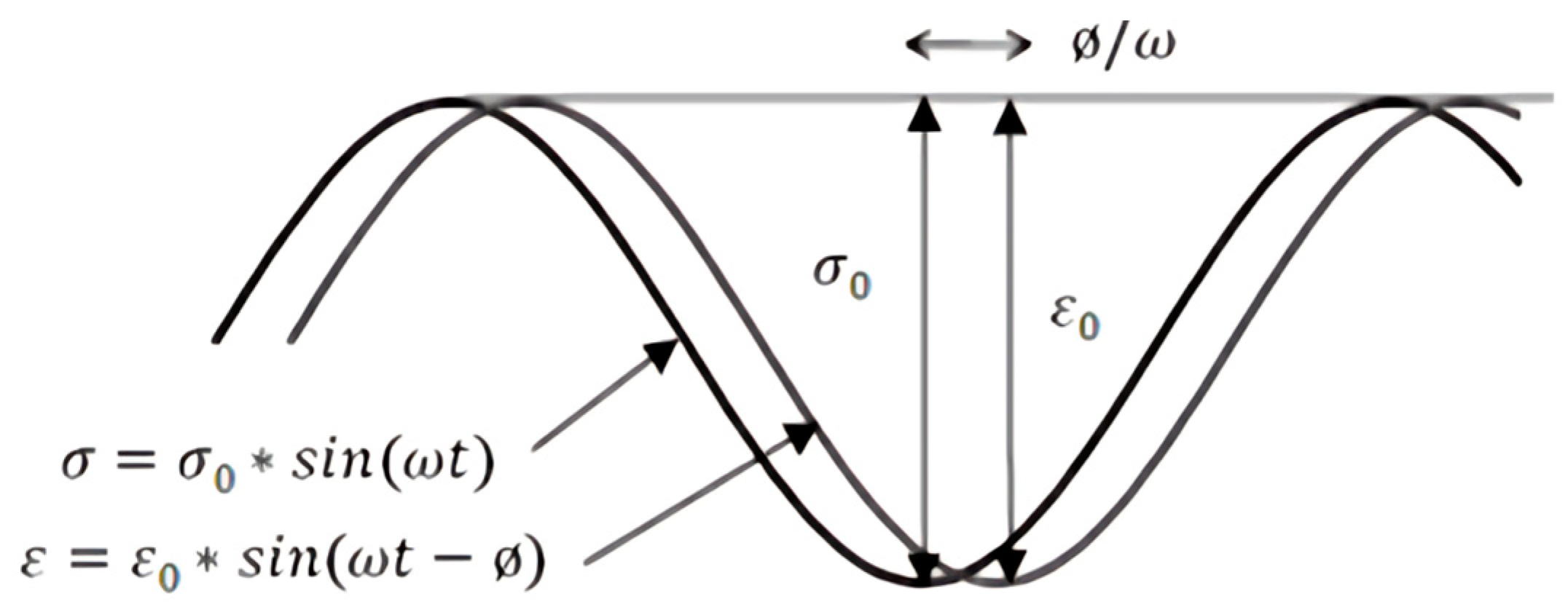
Figure 1. Sinusoidal stress ( σ ) and strain ( ε ) waveform in time ( σ is the stress, σ 0 is the amplitude of the stress, ε is the strain, ε 0 is the amplitude of the strain, ω is the angular frequency of the oscillation, t is the time variable, and ϕ is the phase angle).
Applsci 14 10505 g001
Figure 2. Graphic representation of the dynamic modulus components including the phase angle Φ.
Applsci 14 10505 g002
Figure 3. Parameterization of the sigmoid function [18].
Applsci 14 10505 g003
Figure 4. Generalized Huet–Sayegh rheological model (2S2P1D).
Applsci 14 10505 g004
Figure 6. Isothermal curves of asphalt mixtures with (a) 0% RA, (b) 30% RA, (c) 40% RA, and (d) 50% RA.
Applsci 14 10505 g006
Figure 7. Master curves of asphalt mixtures with 0% RA, 30% RA, 40% RA, and 50% RA.
Applsci 14 10505 g007
Figure 8. Comparison between the master curves of the experimental data and those of the sigmoid function of the asphalt mixture with 0% RA at TR = 20 °C.
Applsci 14 10505 g008
Figure 9. Comparison between the master curves of the experimental data and those of the sigmoid function of the asphalt mixture with 30% RA at TR = 20 °C.
Applsci 14 10505 g009
Figure 10. Comparison between the master curves of experimental data and those of the sigmoid function of the asphalt mixture with 40% RA at TR = 20 °C.
Applsci 14 10505 g010
Figure 11. Comparison between the master curves of experimental data and those of the sigmoid function of the asphalt mixture with 50% RA at TR = 20 °C.
Applsci 14 10505 g011
Figure 12. Comparison between measured |E*|_exp and calculated |E*|_Sigmoid model for the asphalt mixture with 0% RA (the red line represents the identity function y = x).
Applsci 14 10505 g012
Figure 13. Comparison between measured |E*|_exp and calculated |E*|_Sigmoid model for the asphalt mixture with 30% RA (the red line represents the identity function y = x).
Applsci 14 10505 g013
Figure 14. Comparison between measured |E*|_exp and calculated |E*|_Sigmoid model for the asphalt mixture with 40% RA (the red line represents the identity function y = x).
Applsci 14 10505 g014
Figure 15. Comparison between measured |E*|_exp and calculated |E*|_Sigmoid model for the asphalt mixture with 50% RA (the red line represents the identity function y = x).
Applsci 14 10505 g015
Figure 16. Graphical representation of Huet–Sayegh model parameters in (a) Cole–Cole diagram and (b) Black diagram [30].
Applsci 14 10505 g016
Figure 17. Comparison between the master curves of the experimental data and those of the Generalized Huet–Sayegh (2S2P1D) model for asphalt mixture with 0% RA at TR = 20 °C.
Applsci 14 10505 g017
Figure 18. Comparison between the master curves of the experimental data and those of the Generalized Huet–Sayegh (2S2P1D) model for asphalt mixture with 30% RA at TR = 20 °C.
Applsci 14 10505 g018
Figure 19. Comparison between the master curves of the experimental data and those of the Generalized Huet–Sayegh (2S2P1D) model for asphalt mixture with 40% RA at TR = 20 °C.
Applsci 14 10505 g019
Figure 20. Comparison between the master curves of the experimental data and those of the Generalized Huet–Sayegh (2S2P1D) model for asphalt mixture with 50% RA at TR = 20 °C.
Applsci 14 10505 g020
Figure 21. Comparison between measured |E*|_exp and calculated |E*|_2S2P1D model for the asphalt mixture with 0% RA (the green dotted line represents the trend line of the comparison data, and the red line represents the identity function y = x).
Applsci 14 10505 g021
Figure 22. Comparison between measured |E*|_exp and calculated |E*|_2S2P1D model for the asphalt mixture with 30% RA (the green dotted line represents the trend line of the comparison data, and the red line represents the identity function y = x).
Applsci 14 10505 g022
Figure 23. Comparison between measured |E*|_exp and calculated |E*|_2S2P1D model for the asphalt mixture with 40% RA (the green dotted line represents the trend line of the comparison data, and the red line represents the identity function y = x).
Applsci 14 10505 g023
Figure 24. Comparison between measured |E*|_exp and calculated |E*|_2S2P1D model for the asphalt mixture with 50% RA (the green dotted line represents the trend line of the comparison data, and the red line represents the identity function y = x).
Applsci 14 10505 g024
Table 3. Basic used reclaimed asphalt characterization.
Reclaimed Asphalt
Asphalt binder content5.7–5.9%
Asphalt binder propertiesPEN 16 to 24 and softening point 65 to 72 °C
Grading0/8 mm
Table 4. Shift factor determination for asphalt mixtures with different RA contents.
RA (%)0 °C10 °C20 °C30 °C
a(T)log(a(T))a(T)log(a(T))a(T)log(a(T))a(T)log(a(T))
02002.30150.699100.033−1.481
309802.991301.477100.038−1.420
409002.954301.477100.05−1.301
5015003.176301.47710--
Table 5. Regression constants representing the material characteristics (polynomial second degree).
RA (%)Regression Parameters Representing the Material Characteristics
(Polynomial Second Degree)
abc
02.217−0.1300.0003010.98
302.992−0.1540.0002351.00
402.963−0.1560.0004401.00
503.176−0.1810.0011091.00
Table 6. Regression parameters of the sigmoid function.
RA (%)Regression Parameters of the Sigmoid Function
δαβγ
02.3732.032−0.775−0.361
302.4472.087−0.996−0.451
400.0044.451−1.862−0.473
501.3533.149−1.055−0.373
Table 7. Generalized Huet–Sayegh model parameters.
RA (%)Generalized Huet–Sayegh Model Parameters
E0Einfkhαβ
076013,9660.1570.5391.4692,259,955
30115427,7170.2150.7492.7282,259,953
4021426,1050.2420.7253.5592,259,961
501623,9350.1950.6704.6442,259,953
Disclaimer/Publisher’s Note: The statements, opinions and data contained in all publications are solely those of the individual author(s) and contributor(s) and not of MDPI and/or the editor(s). MDPI and/or the editor(s) disclaim responsibility for any injury to people or property resulting from any ideas, methods, instructions or products referred to in the content.