Abstract
In the field of aeronautics, aircraft, as a critical aviation tool, exert a decisive influence on the structural integrity and safety of the entire system. Accurate prediction of the stress field distribution and variations within the aircraft structure is of great importance to ensuring its safety performance. To facilitate such predictions, a rapid assessment method for stress fields based on a multilayer perceptron (MLP) neural network is proposed. Compared to the traditional machine learning algorithm, the random forest algorithm, MLP demonstrates superior accuracy and computational efficiency in stress field prediction, particularly exhibiting enhanced adaptability when handling high-dimensional input data. This method is applied to predict stresses in the wing rib structure. By performing finite element meshing on the wing ribs, the angle of attack, inflow velocity, and node coordinates are utilized as input tensors for the model, enabling it to learn the stress distribution in the wing ribs. Additionally, a peak stress prediction model is separately established for regions experiencing peak stresses. The results indicate that the MAPE of the stress field prediction model is within 5%, with a coefficient of determination R2 exceeding 0.994. For the peak stress model, the MAPE is within 2%, with an R2 exceeding 0.995. This method offers faster computation and greater flexibility, presenting a novel approach for structural strength assessment.
1. Introduction
Airplanes are subjected to complex mechanical loads during flight, influenced by factors such as flight speed, altitude, ambient temperature, and atmospheric pressure. Consequently, stress analysis of aircraft structures is a crucial step in ensuring the overall structural health of the aircraft. The traditional approach to stress analysis involves using finite element method (FEM) software (patran 2018) to simulate the aircraft structure under various operating conditions to obtain the stress field response for corresponding flight scenarios, followed by an evaluation of the aircraft’s structural strength [1,2,3]. While FEM-based methods are effective in capturing changes in the aircraft’s stress field, they are computationally intensive and time-consuming, especially for different aircraft structural models and systems that vary in complexity [4]. The process can become highly resource-demanding. Real-time structural life management requires continuous access to and monitoring of structural stress data, making traditional methods costly and time-prohibitive. Therefore, there is a pressing need to establish a method capable of rapidly predicting the aircraft’s stress conditions to provide effective data support for aircraft structural health monitoring and service life analysis.
With the rapid advancement of artificial intelligence, big data, and information technology, data-driven approaches to structural strength assessment, supported by powerful computational capabilities and vast datasets, have proven highly effective in monitoring the health of structures [5]. For instance, structural health monitoring techniques are employed to continuously track the condition of aircraft structures [6]. This method involves real-time monitoring through advanced sensor networks, which collect structural health data in real time. Signal processing techniques are then used to analyze these signals, enabling the detection of structural conditions, identification of damage or performance degradation, and assessment of the remaining lifespan of the aircraft structure [7].
Broer et al. conducted an analysis of the current state of the art in structural health inspection for aerospace vehicles, identifying two critical aspects of aircraft compliance with the maturity of materials in the structural field. They proposed a multi-sensor data fusion concept and demonstrated a conceptual design study of a fusion-based structural health monitoring (SHM) system. The results indicate that the multi-sensor data fusion concept can significantly benefit condition-based maintenance (CBM) applications in the aircraft industry, particularly in advancing the field of composite aircraft structures [8].
Weijiang et al. developed a nonlinear unsteady aerodynamic model and proposed a theoretical method based on static aeroelasticity, utilizing flight data mining and a fuzzy logic modeling technique. This method assists in the certification of competency holders in aircraft maintenance facilities by enabling them to monitor static aeroelastic behavioral changes and address flight safety warning issues in aging transport aircraft. Additionally, it serves as a valuable tool in structural maintenance programs, enhancing aviation safety as well as operational efficiency [9].
Digital twin technology creates a virtual model of a physical entity by integrating finite element analysis, sensor technology, and visualization techniques. This virtual model enables the simulation, analysis, and prediction of structural behavior, as well as the online and offline monitoring of the structure’s operation. As a result, it facilitates real-time monitoring and management of the aircraft’s structural health, significantly enhancing maintenance and operational decision-making [10].
Lai et al. [11] constructed the measurement-computation combined digital twin (MCC-DT) framework by integrating measurement and computational data. The construction process consists of four key steps. First, an artificial-intelligence-driven load recognition method is employed to identify the loads applied to physical entities, using both measurement and computational data, with two recognition methods proposed: one based on a single-fidelity agent model and the other on deep learning. Second, a multi-fidelity surrogate model (MFS) is applied to enhance the accuracy of the MCC-DT, with two implementation approaches presented, along with an analysis of their respective advantages and disadvantages. Third, an algorithm is developed to estimate cumulative damage to the physical entity in near real time, allowing for damage assessment. Finally, the data generated from the first three steps is integrated into a 3D scene using a web-based graphics library, providing an intuitive visualization of the MCC-DT. An airplane model is used to validate the applicability and effectiveness of this framework [11].
Data prediction methods based on learning algorithms analyze both the linear and nonlinear relationships among input data features, enabling the discovery of underlying correlations between individual features and the prediction of aircraft structural strength [12,13]. Common learning algorithms include clustering, random forests, and neural networks. The primary objective is to understand the data structure and fit it into models that are interpretable and useful for researchers [14,15]. These algorithms are trained on input data sources, employing statistical analysis techniques to generate output values within a specified range. Structural models are then developed from sample data, automating the decision-making process.
Zhen et al. investigated a method for predicting the stress field of a two-dimensional linear elastic cantilever structure using volume data and neural networks. The study employed two distinct prediction architectures: a single-channel input network and a multi-channel input network. By comparing the predictive performance of these models, it was observed that the multi-channel input network exhibited a significantly lower prediction error compared to the single-channel input network. This study indicates that deep learning models could serve as an effective alternative to traditional prediction methods [16].
To provide effective data input for engine turbine disk life management and subsequent engineering applications, Xu et al. developed a turbine disk stress prediction model for aero-engines, leveraging dimensionality reduction and random forest techniques grounded in statistical learning and machine learning methods. The model uses measurable parameters as initial features and performs dimensionality reduction through correlation analysis, principal component analysis, and cluster analysis to extract key control factors. A prediction model is then constructed using the random forest algorithm. The results demonstrate that this approach achieves higher prediction accuracy compared to a random forest model without dimensionality reduction, highlighting its effectiveness in turbine disk stress prediction and its significant technical value for aero-engine life management [17].
Ultrasonic nanocrystalline surface modification (UNSM) is a surface treatment technique that uses ultrasonic vibrational energy to enhance the mechanical properties of materials. The dynamic nature of UNSM induces deformation in the surface and sub-surface layers at very high strain rates, making direct observation of residual stresses and refinement layers challenging. Sembiring et al. proposed an alternative approach using artificial neural networks (ANNs) to predict residual stresses and hardness in various nickel-based alloys treated with UNSM. After training and validating the ANN with experimental data, the model demonstrated strong predictive capability. The study concludes that an ANN can serve as a more accurate alternative in the absence of a mathematical model, providing a useful tool for optimizing UNSM processing parameters [18].
In the design, analysis, and optimization of aerodynamics, flow fields are typically simulated using computational fluid dynamics (CFD). However, CFD simulations are often computationally expensive, memory-intensive, and time-consuming, which limits the exploration of the design space and possibilities for interactive design. Guo et al. employed a convolutional neural network (CNN) to construct an approximate model capable of predicting non-uniform steady laminar flows in 2D or 3D domains in real time, while exploring various geometric representations and network architectures. The results demonstrate that the CNN is two orders of magnitude faster than a GPU-accelerated CFD solver and four orders of magnitude faster than a CPU-based CFD solver in predicting the velocity field, all while maintaining a low error rate. This approach offers a valuable reference for real-time design iterations in the early stages of design development [19].
Wang et al. sought to enhance the full-envelope acceleration performance of a gas turbine engine (GTE) by integrating an input selection strategy (CIS) with a multilayer perceptron (MLP). The CIS strategy is employed to identify the most relevant inputs, which, combined with a weighted integral loss function, results in the design of a highly accurate and robust full-envelope acceleration schedule (FEAS). The MLP further improves the accuracy of the FEAS. Compared to other classical machine learning models, the MLP network demonstrates superior effectiveness in enhancing FEAS accuracy [20].
Wang et al. developed an MLP model for accurately predicting the stress and temperature of a compressor disk using artificial neural network techniques. Engine measurable parameters were used as input for the MLP model, and the back-propagation (BP) neural network algorithm was applied for training. The study also examined the impact of various optimization algorithms on the model’s prediction performance. The results indicate that the model’s predictions are highly consistent with traditional finite element calculations, with relative deviations under 1%, coefficients of determination exceeding 0.95, and root-mean-square errors (JRMSE) within 5. Additionally, the computational time was reduced from hours to minutes or seconds, significantly enhancing the efficiency of the engineering applications. This approach is essential for the life analysis of engine compressor disks and provides a critical foundation for future engineering practices [21].
Existing studies have demonstrated that artificial-neural-network-based modeling methods are increasingly being adopted by scholars in various fields of research. However, there is relatively limited literature in the area of structural stress prediction, where convolutional neural networks (CNNs) are commonly used for prediction modeling. Although CNNs perform well in field prediction tasks, they impose strict requirements on the input and output data structures, which limits the model’s flexibility, particularly when handling unstructured data or multidimensional feature combinations. This increases the complexity of training and the time required. While traditional machine learning methods offer good performance and speed in regression tasks, they face challenges in dealing with complex nonlinear relationships and high-dimensional data, often necessitating intricate feature analysis and processing, which not only increases the workload but can also result in information loss. In the context of aircraft structural health management, real-time, reliable data sources and rapid prediction capabilities are essential.
The MLP possesses strong fitting capabilities and excels at complex nonlinear mapping [22,23]. Compared to other machine learning algorithms, MLP is more adept at capturing intricate nonlinear relationships between input and output when processing high-dimensional data. Additionally, the flexible architecture and numerous adjustable parameters of MLP allow for effective optimization across different application scenarios, making it suitable for adapting to the complex environmental factors and flight conditions encountered by aircraft during operation. However, MLP is highly dependent on data quality and quantity; the presence of noise or incomplete data can reduce prediction accuracy, and insufficient data can lead to overfitting. The ideal application scenario for MLP involves predicting aircraft structural stresses with reliable, high-quality, and sufficient data to ensure model accuracy and reliability. With advancements in big data and health monitoring technologies, the large datasets required for MLP training are increasingly available, supporting its broader application.
To enable rapid prediction of stresses in aircraft structures, this paper establishes a stress prediction model using an MLP neural network, capable of quickly forecasting the stress field. By performing finite element meshing of the wing ribs, the angle of attack, incoming flow velocity, and node coordinates are used as input tensors to the model, allowing it to learn the stress distribution of the wing ribs. The successful application of this model also opens the door for its potential use in predicting stresses in other structural components of the aircraft, such as rotor blades, tail blades, and other wing structures, thereby enhancing the structural safety and reliability of the aircraft.
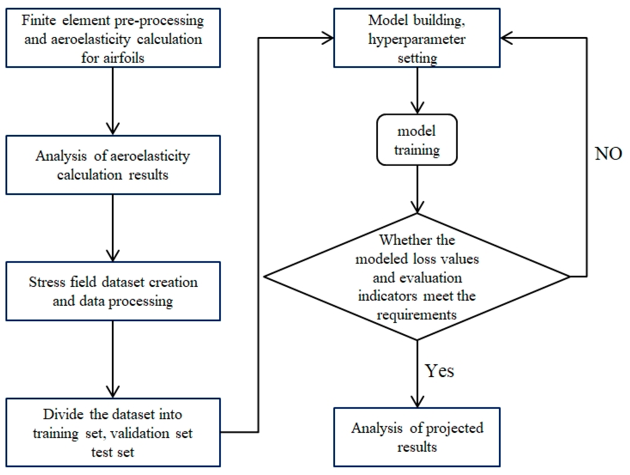
In this study, a finite element model is developed based on the wing design requirements of an air-to-air aircraft. Through the analysis of aerodynamic elasticity results, the equivalent stress distribution patterns of the wing ribs are summarized. A static aerodynamic elasticity calculation is employed to generate a wing rib stress dataset, comprising 173,700 data samples across 300 flight conditions. The MLP neural network is then utilized to construct a prediction model for the wing rib stress field, as well as a model for predicting the peak stress of the wing ribs. The dataset is used for training and prediction. The primary workflow of this paper is illustrated in Figure 1, and the key steps are as follows:
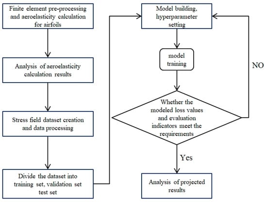
Figure 1.
Data Preparation and Model Workflow.
- Perform finite element modeling and static aerodynamic elasticity calculations of the wing based on the design requirements, followed by an analysis of the stress distribution.
- Establish the wing stress field dataset from the numerical simulation results and divide the dataset into training, validation, and test sets according to standard dataset partitioning practices.
- Identify the input variables for the model and build the MLP model, setting the hyperparameters based on the structure of the input variables. Different hyperparameters are tested to observe the model loss and performance indicators, and the model with the best overall performance is selected to predict the wing’s stress.
- Use common deep learning loss functions and evaluation metrics to assess and fine-tune the model.
- Train the model and compare the predictions of the trained model with those of the RF model for further analysis.
2. Finite Element Modeling and Static Aeroelasticity Calculation for Airfoils
The finite element software Nastran is employed to perform static aerodynamic elasticity calculations on the wing of a composite fixed-wing aircraft currently in the design phase [24,25]. The wing’s design parameters are as follows: a chord length of 1.45 meters, a wingspan of 10.46 meters, and a total airfoil area of 15.167 square meters. According to the design requirements for the air-to-air aircraft, under ultimate load conditions, the vertical displacement of the wing tip must not exceed 6% of the wingspan, and the stress around the bolt holes at the root of the wing beam must not exceed 60% of the material’s compressive strength [26,27].
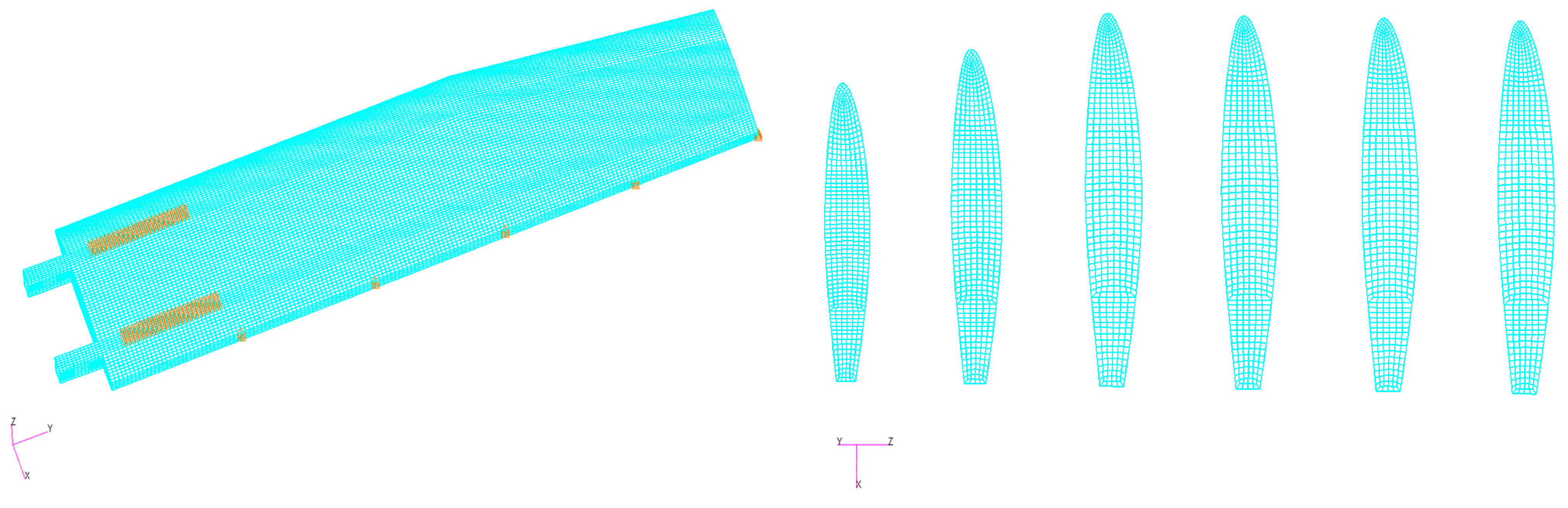
A 3D finite element model of the wing and the wing ribs is shown in Figure 2. Fixed constraints are applied to the bolt holes at the beam root. The wing is meshed using quadrilateral shell cells for the airfoil, wing ribs, and beam. To ensure calculation accuracy, grid independence was verified during the initial design stage using 18,000, 32,000, and 56,000 meshes, with equivalent stress used as the evaluation criterion. For a flight condition of zero altitude, a flight speed of 150 km/h, and an angle of attack of 0°, the grid correlation verification results are shown in Table 1. The findings reveal that the maximum equivalent stress difference between 18,000 and 56,000 grids is less than 2%, indicating that grid independence has been achieved. To reduce computational cost, 32,000 grids are selected for further numerical simulations. The detailed grid cell distribution is presented in Table 2, with the airfoil containing 19,040 cells, the wing ribs containing 3048 cells, and the beam containing 8716 cells. The maximum cell size for the entire wing grid is 27 mm, while the minimum cell size is 2 mm. Based on the design specifications of the aircraft, with flight conditions at zero altitude, a speed range of 150 to 240 km/h, and an angle of attack range of 1 to 10 degrees, the wing stresses are solved under varying conditions.
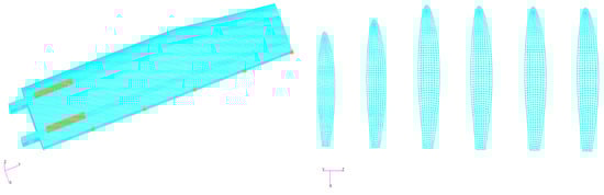
Figure 2.
Structural FEM Model of the Wing.

Table 1.
Grid correlation verification results.
Table 2.
Grid Element Information.
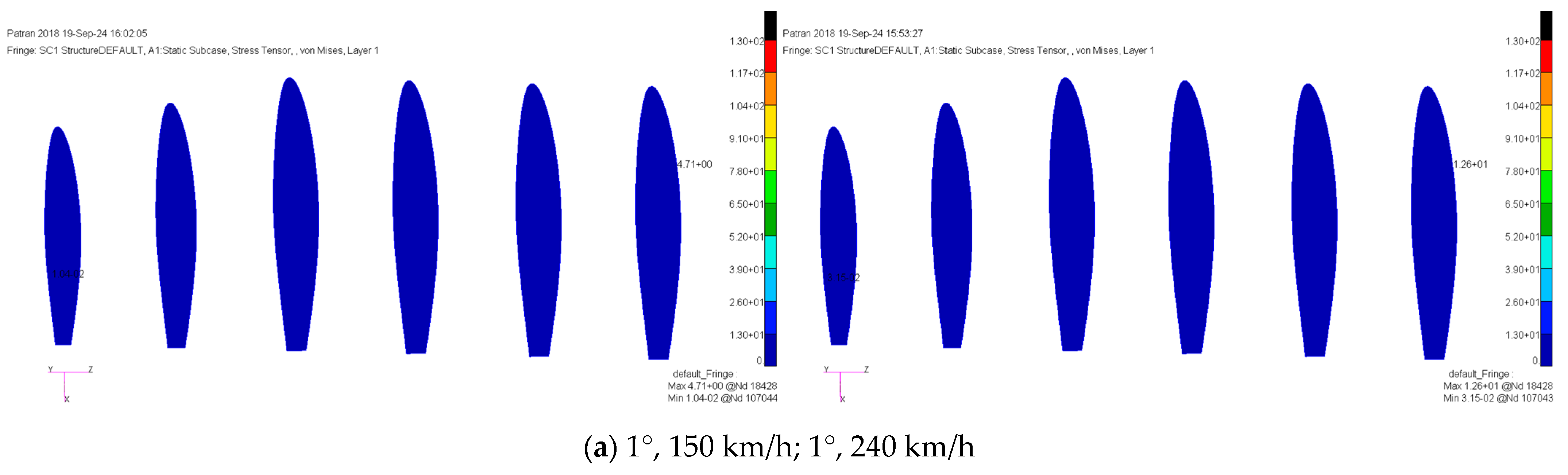
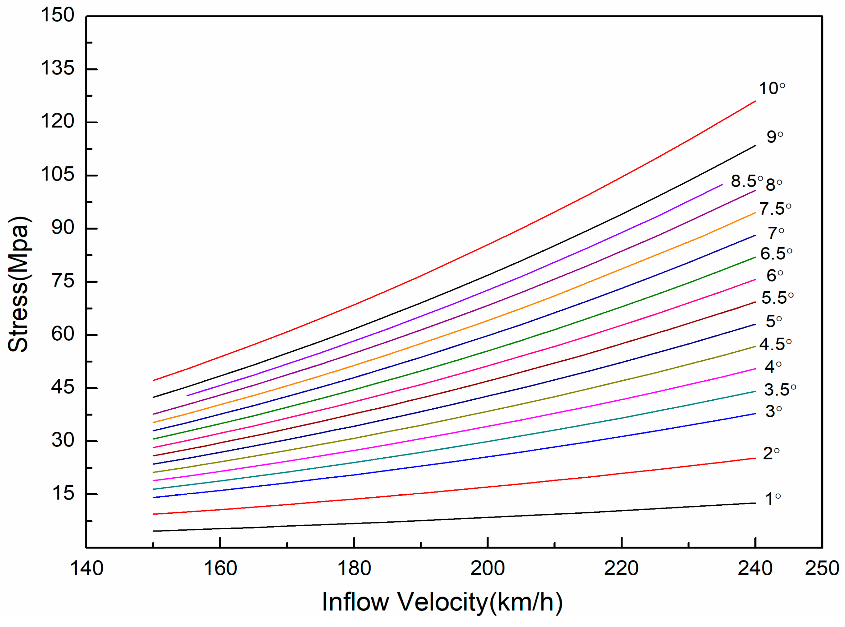
The results for typical working conditions were analyzed, with Figure 3 illustrating the equivalent stress distribution for different angles of attack and flow velocities. The stress distribution in the wing rib is significantly affected by changes in angle of attack and inflow velocity. As these parameters change, the equivalent stress tends to concentrate at the contact points where the wing rib meets the skin and the beam. Stress values increase closer to the wing root, particularly at the contact area between the wing rib, skin, and beam. The peak stress node for the wing rib is at node 18,428 of the first wing rib. Figure 4 shows the stress variation at this node with respect to angle of attack and inflow velocity. At a constant inflow velocity, the equivalent stress at this node increases nonlinearly with the angle of attack. For a fixed angle of attack, the equivalent stress at this node rises with increasing inflow velocity, following an upward trend consistent with observed trends.
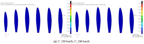
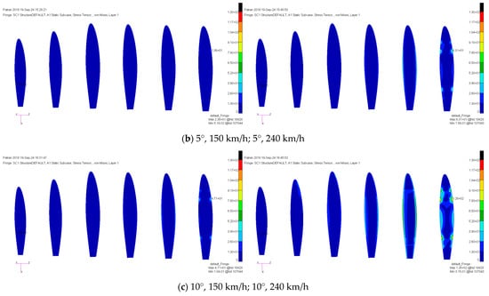
Figure 3.
Simulation Stress Contours at Various Angles of Attack and Inflow Velocities.
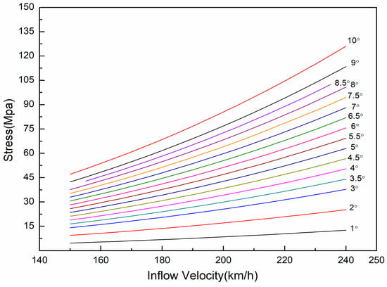
Figure 4.
Nodal stress vs. angle of attack and inflow velocity at node No. 18428.
3. Dataset Creation and Model Variable Definition
3.1. Dataset Creation
Finite element computational data for 300 flight conditions were selected for the wing rib experiencing the highest stress load to establish the stress dataset for this component. The dataset was divided into training, validation, and test sets in an 8:1:1 ratio. To ensure the model can effectively learn the impact of variations in angle of attack and inflow velocity on stress magnitude and distribution, the training and test sets primarily consist of data from angles of attack ranging from 1 to 8 degrees. Additionally, to evaluate the model’s predictive performance under flight conditions not included in the training and validation sets, as well as to address high-load scenarios, data for angles of attack of 9 and 10 degrees were reserved for the test set.
The grid node coordinates of the finite element model of the wing rib, along with the angle of attack and inflow velocity, were used as input parameters for the neural network, while the stress magnitude served as the output. The model evaluation function was employed to compare the predicted stress values with the actual results, thereby assessing the overall performance of the neural network model.
3.2. Model Variables
In structural analysis, node coordinates serve as fundamental information for describing the geometry of a structure. The stress distribution within the structure is influenced by both its geometry and the external loads applied. Consequently, the positional information of the nodes directly impacts the stress distribution. In complex aeronautical structures, abrupt changes in geometry can lead to stress concentrations. In cruise conditions, the stress levels in the wing structure are predominantly influenced by aerodynamic loads, with the angle of attack and inflow velocity being critical parameters affecting the distribution of these loads. To enhance the accuracy of stress magnitude and distribution predictions, node coordinates can be integrated with the angle of attack and inflow velocity. The expressions for the eigenvectors are provided below, and the ranges of the parameters in these eigenvectors are detailed in Table 3.
Table 3.
Model input layer parameters.
In the equation, and represent the node position information, while and denote the angle of attack and flow velocity, respectively. Thus, the stress prediction model can be represented as a function:
In the equation, represents the predicted von Mises stress, is the model function, denotes the model parameters, indicates the weight matrix learned by the model, and is the bias matrix.
4. Model Construction and Result Analysis
4.1. MLP Model Architecture and Hyperparameter Settings
To enhance learning efficiency and accelerate model convergence, it is essential to adjust the input parameters to maintain a similar order of magnitude as the stress data and to normalize the input data. In this study, the MLP model is constructed using TensorFlow version 2.0 within a Conda environment. The model configuration and hyperparameters are detailed in Table 4. The architecture consists of one input layer, one output layer, and ten hidden layers. The input layer contains four nodes, while the output layer has one node. The ReLU activation function is implemented in the hidden layers to improve the network’s nonlinear representation, allowing it to more effectively capture complex feature relationships. Conversely, a linear activation function is utilized in the output layer to ensure the model can produce continuous stress values, thereby yielding accurate prediction results. To mitigate the risk of overfitting due to the high number of neurons, L2 regularization is applied to hidden layers three through ten.
Table 4.
Stress field model structure and hyperparameter settings.
The RMSprop optimizer, known for its superior convergence performance, is selected to enhance the model training process, significantly improving computational efficiency and convergence speed, which aids in finding the optimal solution more quickly. To optimize the overall performance of the model, a grid search is conducted for the learning rate and momentum parameters. Table 5 presents the combinations of momentum parameters and learning rates chosen based on the outcomes of trial calculations and their corresponding scores on the test set. Ultimately, Combination III is selected as the optimal learning rate and momentum parameter pair for the network.
Table 5.
Learning rate and momentum parameter trial scores.
4.2. Random Forest Model
The random forest regression (RF) model is composed of multiple decision trees, each built independently during the training phase. The final prediction is obtained by averaging the predictions from all individual decision trees. To enhance the model’s fitting ability, the data are normalized and standardized. The optimal model and its parameters are identified through a grid search. The grid search intervals and model hyperparameter settings are detailed in Table 6.
Table 6.
RF Model Parameter Settings.
4.3. Loss Function and Evaluation Metrics
In this study, mean squared error (MSE) is utilized as the model’s loss function, and it is defined as follows:
where represents the predicted value from the MLP model, denotes the computed value from the FEM, and is the total number of samples.
To evaluate the model’s performance and explanatory power, three metrics are employed: mean absolute error (MAE), mean absolute percentage error (MAPE), and the coefficient of determination (). These metrics are defined as follows:
where denotes the average of the FEM-calculated values. MAE visualizes the deviation between predicted results and calculated results; MAPE quantifies the extent of deviation between the predicted and calculated results; and measures the proportion of variance in the dependent variable explained by the independent variable, thereby assessing the explanatory power of the statistical model. The integration of these three evaluation metrics provides a comprehensive assessment of the model’s performance.
4.4. Prediction Results and Analysis
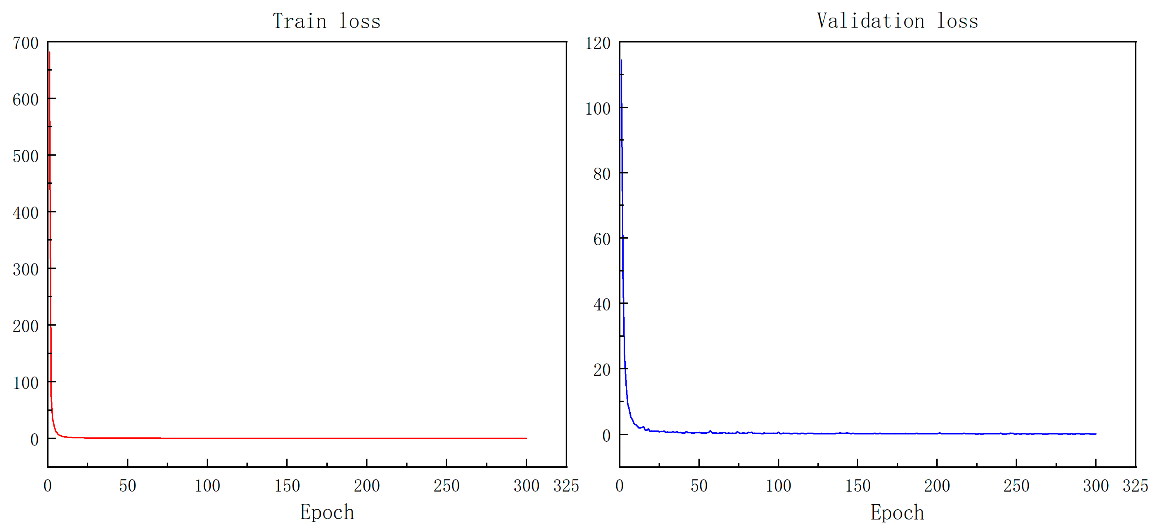
Figure 5 illustrates the decline in loss values for both the training and validation sets. Initially, the loss values decrease rapidly, followed by a gradual reduction as the number of iterations reaches 25 steps. After approximately 90 steps, the loss values stabilize. Following this stabilization, both the training and validation set losses fluctuate within a narrow range without changing by an order of magnitude, indicating that the model has converged. The model updates the network weights using the training data, resulting in significantly lower initial loss for the validation set compared to the training set. To enhance model performance, multiple early stopping criteria are employed to monitor the training process, ensuring that the best model for stress prediction is preserved.
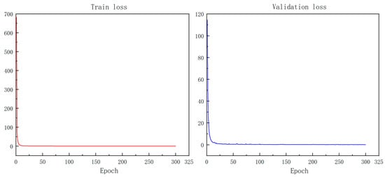
Figure 5.
Training and Validation Loss Curves for MLP Model.
The scores of the MLP model and the RF model on the validation set and test set for each evaluation metric are presented in Table 7. Both models demonstrate a strong fitting performance on the validation set, with MSE metrics below 0.26 MPa, MAE within 0.5 MPa, and MAPE below 5%. In contrast, on the test set, the performance metrics for the MLP model significantly outperform those of the RF model. These results indicate that the MLP model exhibits superior generalization capabilities and a greater ability to capture nonlinear relationships compared to the RF model.
Table 7.
Results of Various Metrics on Validation and Test Sets.
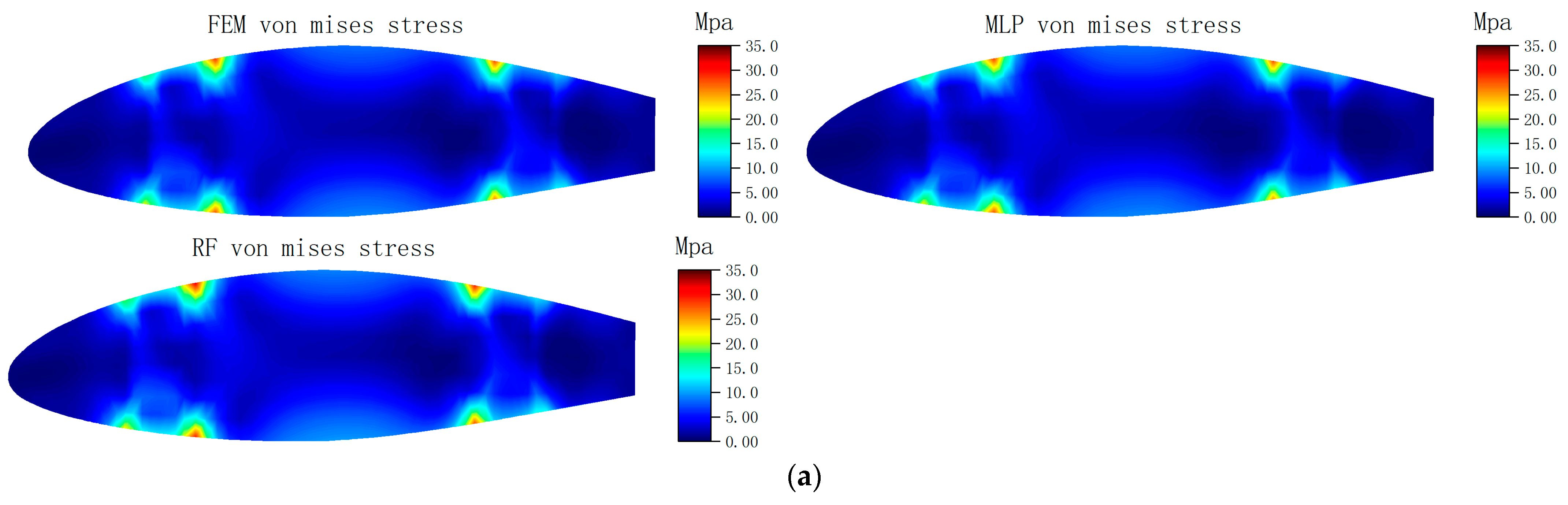
Figure 6 illustrates the stress prediction cloud and relative error cloud for both models under typical working conditions. A comparison of Figure 6a,b reveals that the equivalent stress distribution predictions on the airfoil ribs generated by the MLP model and the RF model align closely with the results obtained from FEM calculations, indicating that both models effectively capture the overall trend. However, Figure 6c,d demonstrate that while the MLP model exhibits lower relative errors compared to the RF model across most regions, some localized areas show relatively large discrepancies when compared to the FEM results.

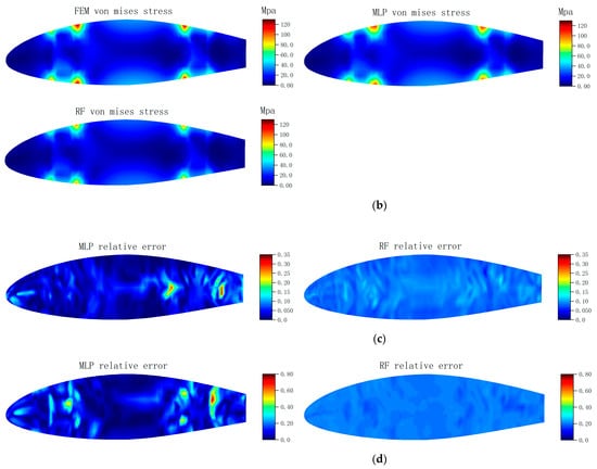
Figure 6.
Stress Prediction Results for Typical Operating Conditions. (a) Angle of Attack: 5°; inflow Velocity: 165 km/h, (b) Angle of Attack: 10°; inflow Velocity: 240 km/h, (c) Angle of Attack: 5°; inflow Velocity: 165 km/h, (d) Angle of Attack: 10°; inflow Velocity: 240 km/h.
This observation can be attributed to the use of MSE as the loss function during the training of the MLP model. This choice tends to produce a more uniform distribution of errors across the overall region, resulting in smaller errors in higher stress areas compared to the true values. The variation in MSE magnitude is influenced by the differences in stress values across regions. Although certain localized areas exhibit errors, the MLP model manages to maintain a low relative error in regions of higher stress, highlighting its strength in handling complex stress distributions.
In summary, based on the analysis of the cloud map results, the MLP model demonstrates superior prediction performance compared to the RF model in high-stress regions, while its performance remains relatively consistent across the overall region. This reflects both its potential and limitations in equivalent stress prediction.
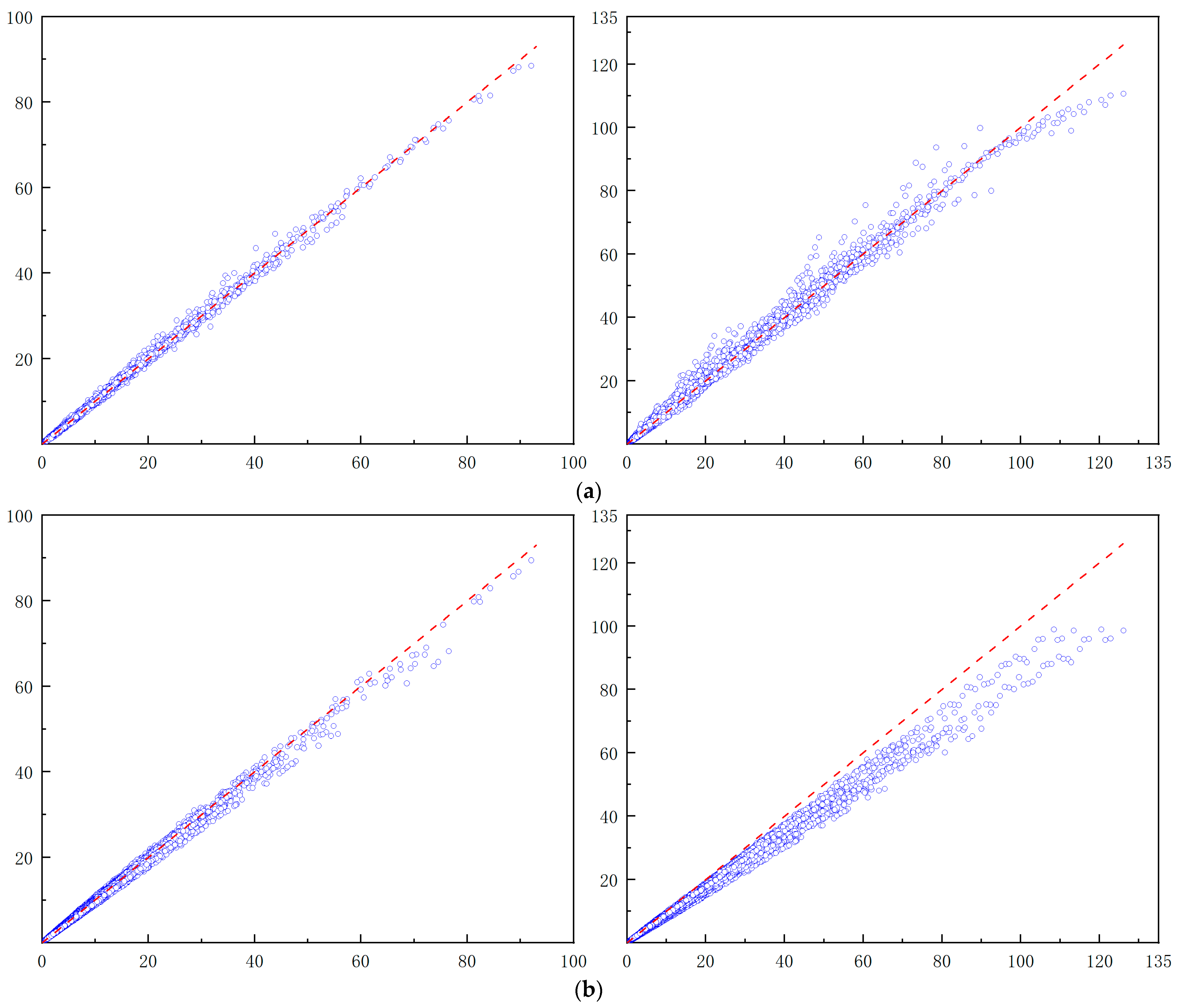
Figure 7 presents scatter plots illustrating the prediction results of the MLP model and the RF model on the training and validation sets. Both models demonstrate strong prediction performance on the validation set; however, the MLP model significantly outperforms the RF model on the test set that includes limit case data. Notably, the prediction error of the RF model on the test set increases as the load rises, particularly after the stress value exceeds 20 MPa. In contrast, the prediction error of the MLP model begins to increase significantly only after the stress value surpasses 100 MPa.
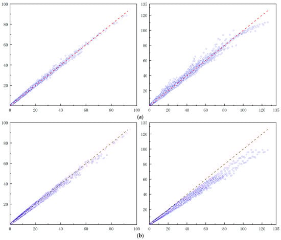
Figure 7.
Scatter Plot of Stress Prediction by MLP Model and RF Model. (a) MLP Model Prediction Results; (b) RF Model Prediction Results.
This discrepancy can be attributed to the nonlinear characteristics exhibited by the variation of loads on the wing ribs as they approach the ultimate operating condition. The MLP model is better equipped to capture these nonlinear dynamics compared to the RF model, which results in a higher threshold for the significant increase in prediction error for the MLP model relative to the RF model.
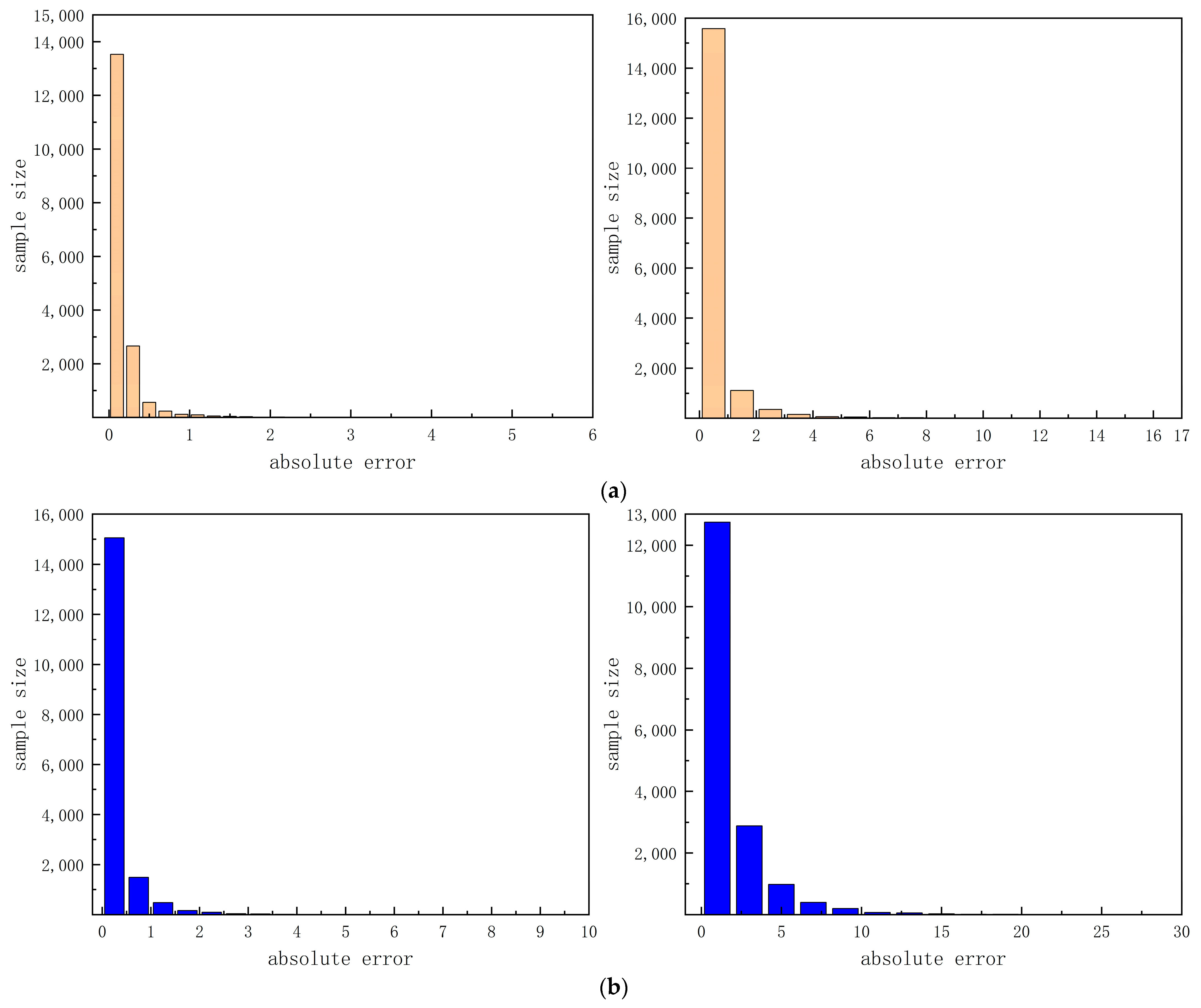
Figure 8 illustrates the distribution of absolute errors for the MLP model and the RF model across the validation and test sets. The MLP model demonstrates strong prediction accuracy on the validation set, with 95% of the regions exhibiting absolute errors of less than 0.6 MPa. However, in the test set, this increases to 95% of the regions showing absolute errors of less than 2 MPa, indicating robust adaptability to new data. In contrast, the RF model also performs well on the validation set, with 95% of the regions having an absolute error of less than 1 MPa. However, in the test set, this increases to 99% of the regions experiencing absolute errors of less than 6 MPa, highlighting its poor adaptability when confronted with unseen data. Consequently, the MLP model consistently outperforms the RF model across both datasets, particularly in handling complex data, demonstrating greater flexibility and stability.
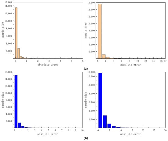
Figure 8.
Absolute Error Distribution for Stress Prediction. (a) Absolute Error Distribution for Validation and Test Sets in MLP Model; (b) Absolute Error Distribution for Validation and Test Sets in RF Model.
4.5. Peak Node Stress Prediction
In engineering practice, the peak value of equivalent stress is particularly critical. Although the wing rib stress field prediction model established in Section 4.4 provides a good overall prediction of the wing rib stress field, the prediction error is somewhat higher in areas of stress concentration. Simulation results indicate that node 18,428 exhibits the maximum stress value on the wing rib. To enhance the accuracy of predicting the equivalent stress peak, an MLP neural network model is developed specifically for stress peak prediction. This model is compared with the RF model. The structure and parameter settings of the MLP model are detailed in Table 8.
Table 8.
Structure and Hyperparameters of Node Prediction Model.
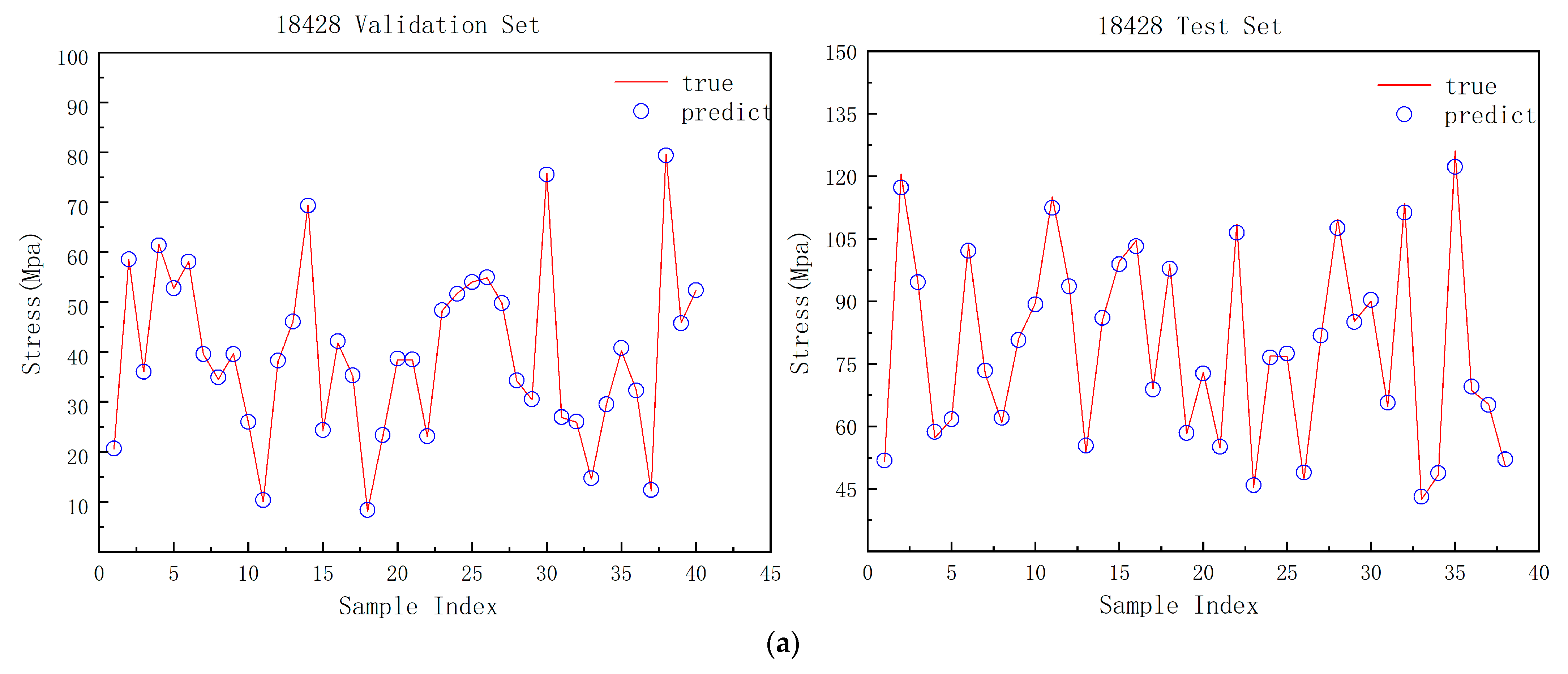
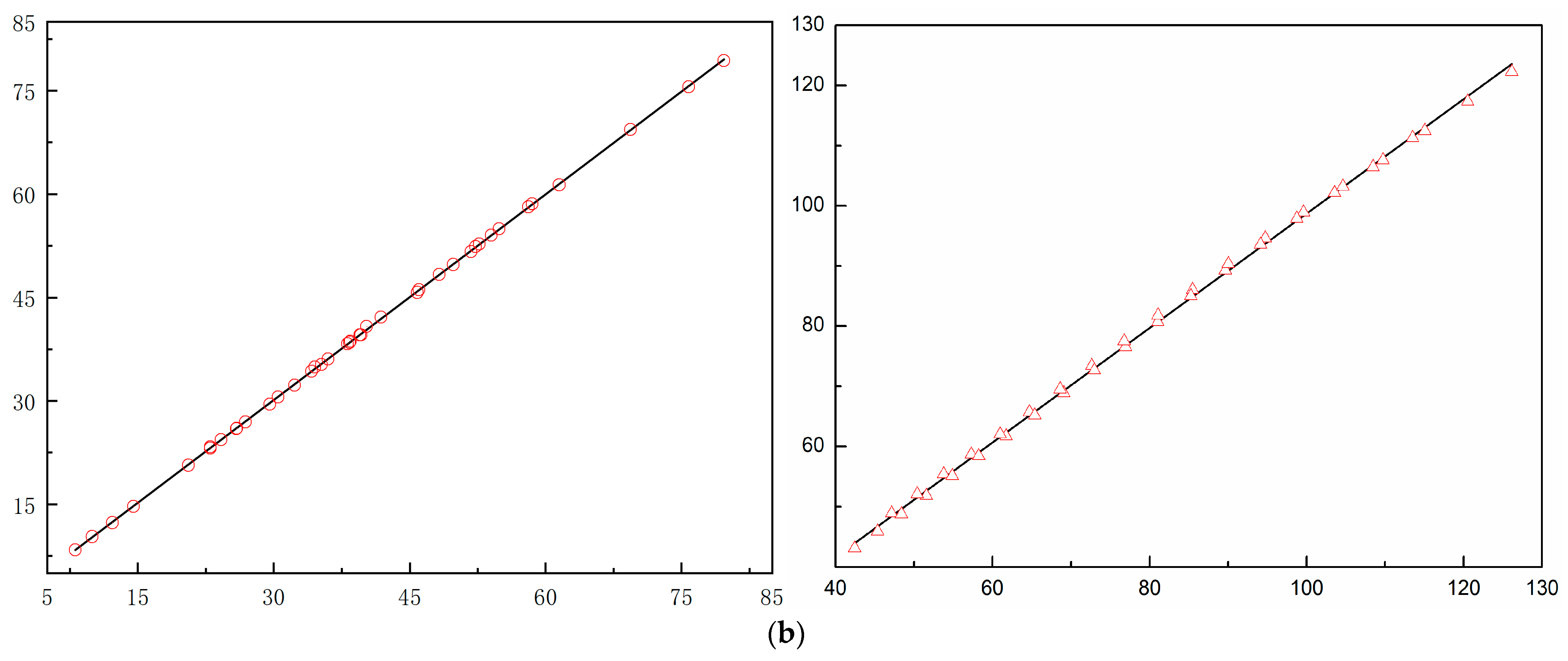
Table 9 presents the scores of the MLP and RF models on the validation and test sets for peak stress prediction. Analysis reveals that the MLP model exhibits a smaller prediction error and significantly higher accuracy compared to the RF model, reflecting its superior fitting ability and complex nonlinear mapping capabilities. Figure 9a illustrates the predictions of the MLP model on the training and test sets, while Figure 9b depicts the regression of peak equivalent force prediction. The correlation coefficients between the peak equivalent force and the MLP-predicted peak equivalent force are 0.999 for the validation set and 0.996 for the test set. The comparison graph and regression plots indicate that, while the MLP model accurately predicts various sizes of equivalent force values on the validation set, larger prediction errors are observed for higher equivalent force values on the test set.
Table 9.
Performance Metrics of MLP and RF Models.
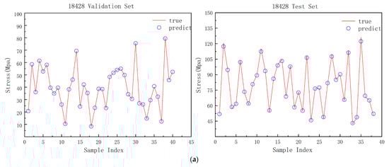
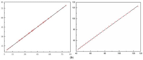
Figure 9.
Peak Stress Prediction Results for MLP Model on Validation and Test Sets. (a) Comparison of Peak Stress Predictions Using MLP; (b) Stress Peak Regression Analysis.
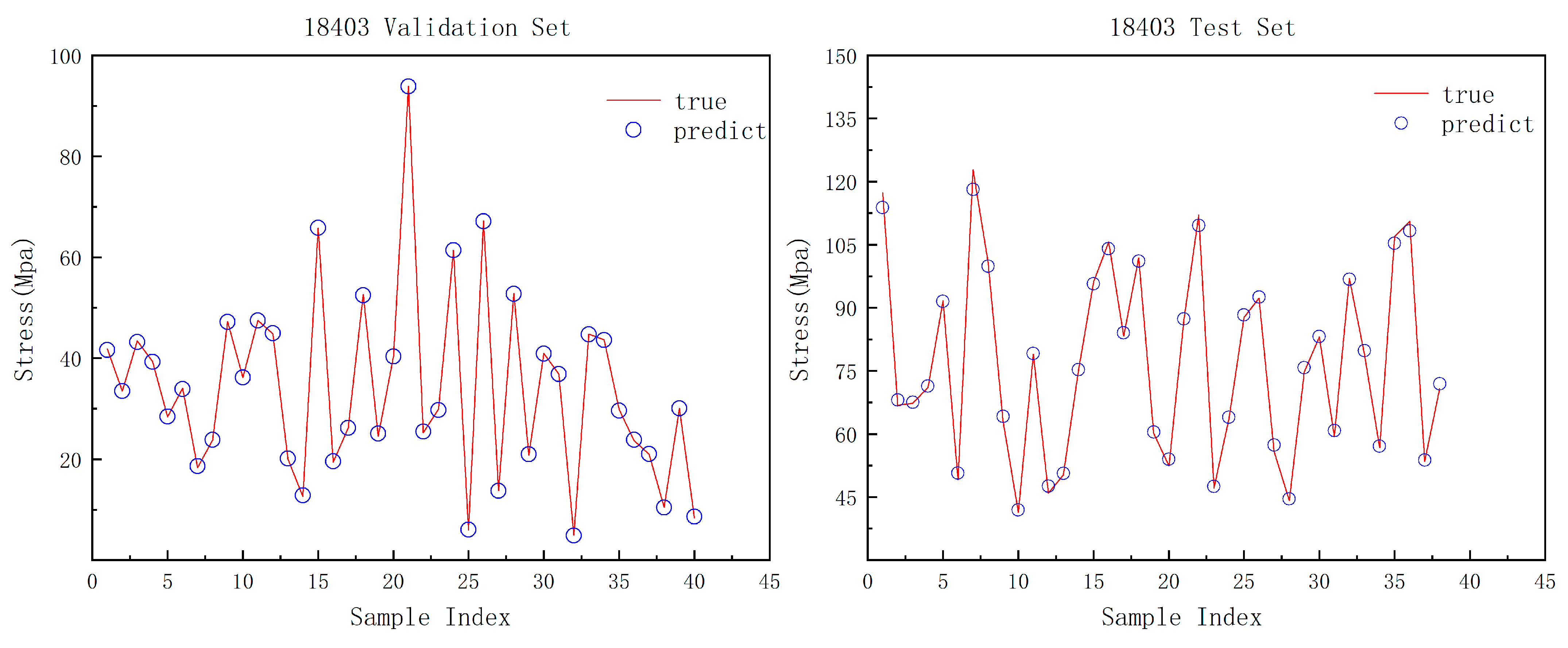
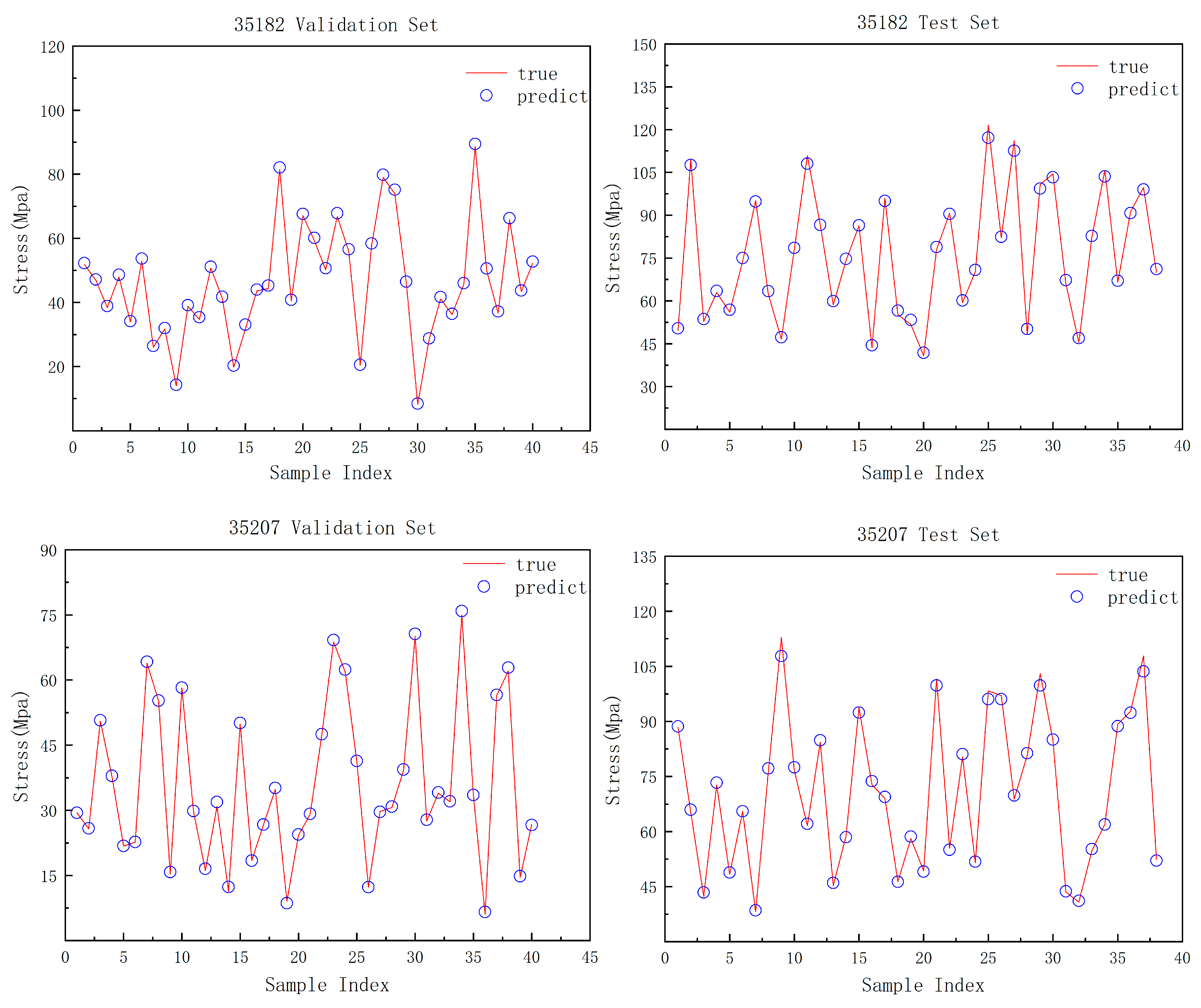
Figure 10 illustrates the stress concentration regions, and based on the FEM simulation results, three nodes (18,403, 35,182, and 35,207) with concentrated equivalent stresses are selected to establish the dataset and predict using the MLP model structure. Table 10 presents the prediction indicators of the MLP model for these different nodes. Figure 11 displays the predictions made by the MLP model for the stress concentration nodes. The MLP model demonstrates excellent performance in predicting the stresses at nodes 18,403, 35,182, and 35,207, reflecting its high accuracy in stress-concentrated regions. For node 18,403, the validation set shows an MSE of 0.026, an MAE of 0.121, and an R2 of 0.999, indicating highly accurate fitting. In the test set, the MSE increases to 1.908 and the MAE to 0.982, yet the model maintains a high level of accuracy despite this increase. For node 35,182, the validation set records an MSE of 0.344, an MAE of 0.519, and an R2 of 0.998, again demonstrating strong predictive power. The test set results show an MSE of 1.986 and an MAE of 1.108, which remain within acceptable limits. At node 35207, the validation set has an MSE of 0.152 and an MAE of 0.290, reflecting high prediction accuracy, while the test set performs with an MSE of 1.956 and an MAE of 0.875.
Figure 10.
Areas of Equivalent Stress Concentration.
Table 10.
Results of Various Indicators for Stress Prediction Models at Each Node.
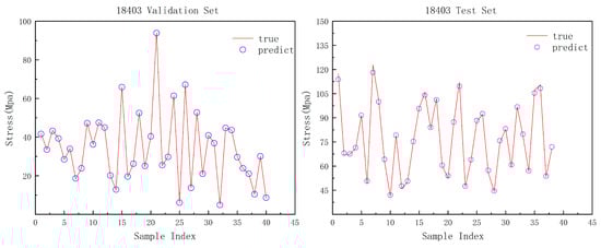
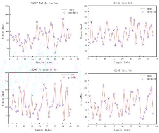
Figure 11.
Prediction Results for Nodes 18,403, 35,182, and 35,207.
Across all three nodes, the MLP model not only delivers accurate stress predictions under extreme load conditions but also maintains stable overall performance, demonstrating its validity and reliability in addressing complex mechanical challenges. These results collectively confirm the efficiency of the MLP model in predicting stress-concentrated regions.
5. Conclusions
In this paper, in order to realize the prediction of the stress field of aircraft structure, a fast assessment method of the stress field based on an MLP neural network is proposed, and the stress prediction of the wing rib structure is carried out by this method. In this paper, the wing aeroelasticity calculation results are analyzed to summarize the wing stress distribution law and establish the wing rib stress field dataset. The MLP model is trained so that the model can accurately realize the prediction of the equivalent stress field, and the accuracy level of the MLP model is verified by analyzing the prediction data of the validation set and test set in combination with the evaluation index and the equivalent stress prediction cloud diagram. By comparing with the RF model, the powerful fitting ability and adaptability of the MLP model are demonstrated. The following conclusions were obtained by summarizing the work:
- (1)
- In this paper, we propose a method that involves finite element meshing of the wing ribs and using node information along with the angle of attack and inflow velocity as the input tensor for the model. This approach enables the model to learn the stress distribution of the wing ribs and establishes a separate prediction model for the peak stress region. The results demonstrate that this method effectively establishes a robust mapping relationship between node information and stress distribution, maintains high flexibility in network inputs without requiring a fixed data size, and achieves high prediction accuracy.
- (2)
- Compared with traditional machine learning algorithms like the RF model, the MLP demonstrates higher accuracy and computational efficiency in stress field prediction. The MLP particularly exhibits stronger adaptability when handling high-dimensional input data. In this study, the prediction performance of the MLP model is contrasted with that of the RF algorithm. Both models show commendable prediction performance on the validation set; however, the MLP model significantly outperforms the RF model on the test set, which includes extreme-condition data. The prediction error of the RF model on the test set increases with load, notably rising after the stress value exceeds 20 MPa. In contrast, the prediction error of the MLP model remains relatively stable until the stress value reaches 100 MPa. This difference can be attributed to the nonlinear characteristics of the load variations on the wing ribs as they approach ultimate operating conditions. The MLP model is more adept at capturing these nonlinear relationships than the RF model, resulting in a higher threshold for significant increases in prediction error. Overall, the results underscore the MLP’s superiority in adapting to complex, high-dimensional data and handling nonlinear relationships in stress predictions, particularly under extreme loading conditions.
- (3)
- Analysis of the stress field prediction results reveals that the MLP models achieve the following metrics on the validation set: MSE within 0.09 MPa, MAE within 0.16 MPa, MAPE within 5%, and R2 above 0.999. On the test set, the models achieve MSE within 0.998 MPa, MAE within 0.5 MPa, MAPE within 5%, and R2 above 0.99.
- (4)
- A peak stress prediction model is established separately for nodes with peak stress and stress concentration, enhancing the accuracy of peak equivalent stress predictions. In the validation set, the model achieves MSE within 0.035 MPa, MAE within 0.13 MPa, MAPE within 0.504%, and R2 above 0.999. In the test set, the model achieves MSE within 1.8 MPa, MAE within 0.998 MPa, MAPE within 1.25%, and R2 above 0.99. Compared to the stress field prediction model, the peak stress prediction model shows higher MSE and MAE but lower MAPE. This difference may be attributed to the fact that the MSE and MAE metrics in the stress field model are averaged across all nodes, whereas the peak dataset is smaller, which may lead to incomplete capture of the mapping relationship between features and target values.
The MLP neural-network-based stress prediction method proposed in this paper effectively maps node position and flight parameter information to stress. Finite element calculations for a single case take approximately 7 min, whereas the stress field prediction model completes data predictions for 30 flight cases in just 2 s. This results in a significantly faster computation speed compared to traditional finite element methods. The single-output structural characteristics of the network enhance its power and flexibility, offering a novel approach to structural strength assessment. However, there are still the following shortcomings in this work:
- (1)
- The applicability of the prediction model for the airfoil rib structure requires further enhancement, specifically in enabling the MLP model to comprehensively account for the effects of variations in airfoil shape on stress distribution. To improve the model’s applicability to the airfoil rib structure, it is essential to incorporate stress distribution data from various airfoil types. The MLP model proposed in this study currently addresses only a single airfoil type, indicating potential areas for further development.
- (2)
- Additionally, the application of the prediction model to other structural components necessitates expansion. The distribution of structural stress is intricately linked to the inherent characteristics of each structure; thus, evaluating the model’s applicability involves assessing its performance across diverse structural types. The MLP model presented herein has solely been implemented for the wing rib structure, and its applicability to other structural locations warrants further investigation.
Future research should aim to extend the application of the developed models systematically across a broader range of aircraft structures. This includes integrating additional structural parameters within the same framework to enhance the model’s applicability to those structures. Furthermore, existing knowledge in deep learning and structural mechanics should be leveraged to refine the data learning process and construct a more explanatory network structure that elucidates the mechanisms underlying stress generation.
Author Contributions
W.J.: conceptualization, investigation, resources, supervision, project administration, writing—original draft, writing—review and editing; Q.C.: conceptualization, investigation, data curation, funding acquisition, writing—original draft, writing—review and editing. All authors have read and agreed to the published version of the manuscript.
Funding
The authors are grateful for financial support from the Science Fund for Distinguished Young Scholars of Chongqing Municipality (CSTB2022NSCQ JQX0024).
Institutional Review Board Statement
Not applicable.
Informed Consent Statement
Not applicable.
Data Availability Statement
The data presented in this study are available on request from the corresponding author.
Conflicts of Interest
The authors declare no conflicts of interest.
References
- Giannella, V.; Vivo, E.; Mazzeo, M.; Citarella, R. FEM-DBEM Approach to Simulate Crack Propagation in a Turbine Vane Segment Undergoing a Fatigue Load Spectrum. Procedia Struct. Integr. 2018, 12, 479–491. [Google Scholar] [CrossRef]
- Cunha, F.; Dahmer, M.; Chyu, M. Thermal-Mechanical Life Prediction System for Anisotropic Turbine Components. J. Turbomach. 2006, 128, 240–250. Available online: https://asmedigitalcollection.asme.org/turbomachinery/article-abstract/128/2/240/470626/Thermal-Mechanical-Life-Prediction-System-for?redirectedFrom=fulltext (accessed on 28 May 2024). [CrossRef]
- Ma, Y.; Shi, B.; Ali, L.; Bai, Y.; Fang, P. Mechanical Analysis of a Type of Wire Rope Subjected to Tension. Ships Offshore Struct. 2024, 19, 541–547. Available online: https://www.tandfonline.com/doi/full/10.1080/17445302.2023.2190445 (accessed on 28 May 2024). [CrossRef]
- Zhang, F.; Kim, M.Y. A Nonlinear FE Formulation for Elastic Buckling and Post-Buckling Analysis of Pre-Stressed Stayed Columns with Bonded/Un-Bonded Cable Stays. Thin-Walled Struct. 2024, 199, 111760. Available online: https://www.semanticscholar.org/paper/A-Nonlinear-FE-formulation-for-Elastic-Buckling-and-Zhang-Kim/bcd9341d8d0604c40cfa29de23e5280a5164ac1e (accessed on 28 May 2024). [CrossRef]
- Tao, F.; Qi, Q. New IT Driven Service-Oriented Smart Manufacturing: Framework and Characteristics. IEEE Trans. Syst. Man Cybern. Syst. 2019, 49, 81–91. [Google Scholar] [CrossRef]
- Claus, R.O.; Gunther, M.F.; Wang, A.; Murphy, K.A. Extrinsic Fabry-Perot Sensor for Strain and Crack Opening Displacement Measurements from −200 to 900 Degrees C. Smart Mater. Struct. 1992, 1, 237. Available online: https://iopscience.iop.org/article/10.1088/0964-1726/1/3/008 (accessed on 28 May 2024). [CrossRef]
- Zhang, Y.; Wang, B.; Ning, Y.; Xue, H.; Lei, X. Study on Health Monitoring and Fatigue Life Prediction of Aircraft Structures. Materials 2022, 15, 8606. Available online: https://www.mdpi.com/1996-1944/15/23/8606 (accessed on 28 May 2024). [CrossRef]
- Broer, A.A.; Benedictus, R.; Zarouchas, D. The Need for Multi-Sensor Data Fusion in Structural Health Monitoring of Composite Aircraft Structures. Aerospace 2022, 9, 183. Available online: https://www.mdpi.com/2226-4310/9/4/183 (accessed on 28 May 2024). [CrossRef]
- Jiang, W.; Chang, R.C.; Zhang, S.; Zang, S. Structural Health Monitoring and Flight Safety Warning for Aging Transport Aircraft. J. Aerosp. Eng. 2023, 36, 04023059. Available online: https://ascelibrary.org/doi/10.1061/JAEEEZ.ASENG-4740 (accessed on 28 May 2024). [CrossRef]
- Dong, L.; Zhou, X.; Zhao, F.; He, S.; Lu, Z.; Feng, J. Key technologies for modeling and simulation of airframe digital twin. Acta Aeronaut Astronaut. Sin. 2020, 42, 23981. (In Chinese) [Google Scholar] [CrossRef]
- Lai, X.; Yang, L.; He, X.; Pang, Y.; Song, X.; Sun, W. Digital Twin-Based Structural Health Monitoring by Combining Measurement and Computational Data: An Aircraft Wing Example. J. Manuf. Syst. 2023, 69, 76–90. [Google Scholar] [CrossRef]
- Liu, H.; Ma, T.; Lin, Y.; Peng, K.; Hu, X.; Xie, S.; Luo, K. Deep Learning in Rockburst Intensity Level Prediction: Performance Evaluation and Comparison of the NGO-CNN-BiGRU-Attention Model. Appl. Sci. 2024, 14, 5719. Available online: https://www.mdpi.com/2076-3417/14/13/5719 (accessed on 21 September 2024). [CrossRef]
- An, L.; Dias, D.; Carvajal, C.; Peyras, L.; Breul, P.; Jenck, O.; Guo, X. Pore Water Pressure Prediction Based on Machine Learning Methods—Application to an Earth Dam Case. Appl. Sci. 2024, 14, 4749. Available online: https://www.mdpi.com/2076-3417/14/11/4749 (accessed on 21 September 2024). [CrossRef]
- Yu, T.; Wu, X.; Yu, Y.; Li, R.; Zhang, H. Establishment and Validation of a Relationship Model between Nozzle Experiments and CFD Results Based on Convolutional Neural Network. Aerosp. Sci. Technol. 2023, 142, 108694. [Google Scholar] [CrossRef]
- Lee, D.H.; Lee, D.; Han, S.; Seo, S.; Lee, B.J.; Ahn, J. Deep Residual Neural Network for Predicting Aerodynamic Coefficient Changes with Ablation. Aerosp. Sci. Technol. 2023, 136, 108207. [Google Scholar] [CrossRef]
- Nie, Z.; Jiang, H.; Kara, L.B. Stress Field Prediction in Cantilevered Structures Using Convolutional Neural Networks. J. Comput. Inf. Sci. Eng. 2020, 20, 011002. Available online: https://asmedigitalcollection.asme.org/computingengineering/article-abstract/20/1/011002/955168/Stress-Field-Prediction-in-Cantilevered-Structures?redirectedFrom=fulltext (accessed on 28 May 2024). [CrossRef]
- Xu, J.; Wang, X.; Qing, H.; He, Y. Stress Prediction of Aero-Engine Turbine Disk Based on Dimension Reduction and Random Forest. J. Propuls. Technol. 2023, 44, 146–154. Available online: https://wf.pub/perios/article:tjjs202312014 (accessed on 21 September 2024). (In Chinese).
- Sembiring, J.P.B.A.; Amanov, A.; Pyun, Y.S. Artificial Neural Network-Based Prediction Model of Residual Stress and Hardness of Nickel-Based Alloys for UNSM Parameters Optimization. Mater. Today Commun. 2020, 25, 101391. [Google Scholar] [CrossRef]
- Guo, X.; Li, W.; Iorio, F. Convolutional Neural Networks for Steady Flow Approximation. In Proceedings of the 22nd ACM SIGKDD International Conference on Knowledge Discovery and Data Mining, San Francisco, CA, USA, 13–17 August 2016; Available online: https://dl.acm.org/doi/10.1145/2939672.2939738 (accessed on 28 May 2024).
- Wang, K.; Xu, M.; Li, M.; Geng, J.; Liu, J.; Song, Z. A Multi-Input Based Full Envelope Acceleration Schedule Design Method for Gas Turbine Engine Based on Multilayer Perceptron Network. Aerosp. Sci. Technol. 2022, 130, 107928. [Google Scholar] [CrossRef]
- Wang, X.M.; Xu, J.P.; He, Y. Stress and temperature prediction of aero-engine compressor disk based on multilayer perceptron. IEEE J. Aerosp. Power 2024, 10, 205–214. Available online: https://qikan.cqvip.com/Qikan/Article/Detail?id=7111840638 (accessed on 12 October 2024). (In Chinese).
- Kruse, R.; Mostaghim, S.; Borgelt, C.; Braune, C.; Steinbrecher, M. Multi-Layer Perceptrons. In Computational Intelligence; Springer: Cham, Switzerland, 2022; pp. 53–124. ISBN 978-3-030-42227-1. [Google Scholar]
- Tang, J.; Deng, C.; Huang, G.B. Extreme Learning Machine for Multilayer Perceptron. IEEE Trans. Neural Netw. Learn. Syst. 2015, 27, 809–821. Available online: https://ieeexplore.ieee.org/document/7103337 (accessed on 28 May 2024). [CrossRef] [PubMed]
- McGurk, M.; Stodieck, O.; Yuan, J. Probabilistic Aeroelastic Analysis of High-Fidelity Composite Aircraft Wing with Manufacturing Variability. Compos. Struct. 2024, 329, 117794. [Google Scholar] [CrossRef]
- Kumar, S.; Onkar, A.K.; Manjuprasad, M. A Study on Stochastic Aeroelastic Stability and Flutter Reliability of a Wing. Acta Mech. 2023, 234, 6649–6675. Available online: https://link.springer.com/article/10.1007/s00707-023-03727-8 (accessed on 28 May 2024). [CrossRef]
- Olejnik, A.; Kachel, S.; Rogólski, R. Techniques for Adjusting Qualities of Aircraft Structural Models for More Effective Aeroelastic Flutter Analyses. J. Phys. Conf. Ser. 2023, 2526, 012040. Available online: https://iopscience.iop.org/article/10.1088/1742-6596/2526/1/012040 (accessed on 28 May 2024). [CrossRef]
- Chen, Q.; Han, J.; Yun, H. Effect of Engine Thrust on Nonlinear Flutter of Wings. J. Vibroeng. 2013, 15, 1731–1739. [Google Scholar]


Disclaimer/Publisher’s Note: The statements, opinions and data contained in all publications are solely those of the individual author(s) and contributor(s) and not of MDPI and/or the editor(s). MDPI and/or the editor(s) disclaim responsibility for any injury to people or property resulting from any ideas, methods, instructions or products referred to in the content. |
© 2024 by the authors. Licensee MDPI, Basel, Switzerland. This article is an open access article distributed under the terms and conditions of the Creative Commons Attribution (CC BY) license (https://creativecommons.org/licenses/by/4.0/).