Abstract
Over the past decade, the development of computer-aided detection tools for medical image analysis has seen significant advancements. However, tasks such as the automatic differentiation of tissues or regions in medical images remain challenging. Magnetic resonance imaging (MRI) has proven valuable for early diagnosis, particularly in conditions like prostate cancer, yet it often struggles to produce high-resolution images with clearly defined boundaries. In this article, we propose a novel segmentation approach based on minimum cross-entropy thresholding using the equilibrium optimizer (MCE-EO) to enhance the visual differentiation of tissues in prostate MRI scans. To validate our method, we conducted two experiments. The first evaluated the overall performance of MCE-EO using standard grayscale benchmark images, while the second focused on a set of transaxial-cut prostate MRI scans. MCE-EO’s performance was compared against six stochastic optimization techniques. Statistical analysis of the results demonstrates that MCE-EO offers superior performance for prostate MRI segmentation, providing a more effective tool for distinguishing between various tissue types.
1. Introduction
Image processing of medical images has become an exciting research topic due to its importance in the detection, diagnosis, and staging of health conditions. Medical images cover a wide range of technologies designed to generate a visual representation of internal morphology or function with the specific purpose of assisting health care practitioners. Many technologies utilize non-invasive approaches, such as magnetic resonances (MR), ultrasonography, and positron emission tomography (PET), among others. From these alternatives, MR images (MRIs) are often used to analyze anatomical structures as they provide high spatial distribution. However, the acquisition of high-quality MRIs is quite challenging, since MRIs are known to suffer from movements of the patient and the presence of artifacts [1], which can compromise the quality of the scans and subsequently the accuracy of diagnoses and treatment plans. These challenges necessitate the use of advanced techniques for image segmentation, which is a crucial step in interpreting medical images and assisting in diagnosis, particularly in diseases like prostate cancer, which is the second most common and deadly cancer in men after lung cancer [2]. Prostate cancer is known for its silent development, and it is often diagnosed at an advanced stage. According to global cancer statistics from 2022, 1,466,680 new cases of prostate cancer were diagnosed that year [3]. Early detection is crucial, as it significantly improves survival rates; however, challenges in this area remain, due to the subtle nature of early-stage tumors in imaging. Accurate analysis of prostate MRIs is therefore essential to improving diagnostic accuracy and reducing the need for invasive biopsies.
The use of computer-aided diagnostic tools (CAD) as a complementary means to medical imaging can help health practitioners to avoid or reduce biopsy rates while also saving time [4]. Research around the design of CAD centers on three main topics: denoising, segmentation, and classification.
Segmentation is a fundamental task in medical image processing and plays a critical role in separating different regions of interest within an image, especially when the boundaries are not clearly defined [5]. Traditional segmentation methods, such as thresholding, offer simplicity but face limitations in the context of complex medical images, particularly when distinguishing between subtle tissue variations in MRI scans. Thresholding stands as a simple yet powerful methodology meant to separate two or more regions of an image. This approach first transforms a given image into a frequency representation over an intensity histogram. The histogram is the input of thresholding methods, while the core idea is to find a threshold value () that accurately divides the histogram into two or more classes. Each class will homogeneously share the same intensity value. Traditionally, thresholding approaches have been named bilevel or multilevel thresholding (MTH) according to the number of thresholds that the implementation possesses. The solution of a MTH problem involves the finding of the optimal threshold values () that segment a given image properly. As the number of thresholds increases, so does the computational complexity of the task; thus, the efficient selection of threshold values is a non-trivial task. In the literature, we can find numerous approaches to determine the best threshold values for an image. First, the work proposed by Ostu used the between-class variance as a non-parametric criterion [6]. Entropy-based approaches take information theory elements to determine if a given partition of a histogram is good enough. This area started with the basic formulation of the Shannon entropy [7], followed by a multitude of variants, including Kapur [8], Tsallis [9], Renyi [10], and cross-entropy [11]. Cross-entropy has been largely adopted by the image processing community since it was proposed by Li and Lee, and it is often referred to as minimum cross-entropy criterion (MCE). The approaches that make use of MCE can determine if a particular set of thresholds minimizes the cross-entropy of the histogram’s partition. Therefore, MCE is just an entropic criterion, not a whole methodology for thresholding by itself. MCE could be used in an exhaustive search to evaluate all possible combinations of threshold values, but this is, of course, impractical. To alleviate the computational burden of such a kind of search, stochastic optimization algorithms (SOAs) are often applied to this task. SOAs use stochasticity in their operators to help to find optimal solutions to complex problems in reasonable times. We can see in the literature multiple approaches that employ randomness and domain-specific rules that help to identify optimal solutions quickly, and they are often referred to as metaheuristic algorithms. We can find examples of SOAs applied to the multilevel thresholding of images in [12,13,14,15,16,17,18]. Specific to the field of health care, we can find a plethora of implementations. For instance, we can find a modification of the Slime Mould Algorithm (SMA) used to perfom image thresholding over breast thermograms [19]. Ref. [20] uses a variant of the manta ray foraging optimization algorithm (MRFO) to segment computer tomographies (CT) from COVID-19 patients using Otsu as the objective function. Avalos et al. proposed an accurate cluster chaotic optimization approach for digital mammograms, lymphoblastic leukemia images, and brain MRIs using cross-entropy as the non-parametric criterion [21]. Panda et al. presented a hybrid algorithm called the hybrid adaptive cuckoo search-squirrel search algorithm (ACS-SSA) to segment T-2 weighted axial brain MR images [22]. Houssein et al. used a modification of the chimp optimization algorithm (COA) for the segmentation of breast thermographic images [23].
Despite these advances, challenges remain in achieving both high accuracy and computational efficiency in medical image segmentation. The balance between exploration and exploitation in SOAs is critical for their success in specific applications, but it is not always straightforward to adapt general-purpose algorithms to the domain of medical imaging. Moreover, the performance of these algorithms is highly dependent on the problem at hand, making it necessary to assess their applicability in the context of specific medical conditions and imaging modalities. SOAs and specifically metaheuristic algorithms are often presented in the academic literature using a set of standard benchmark functions designed to stress the algorithm and to determine if the proposed approach is better than previous approaches in a general sense. Although usual comparisons give us a glimpse of the algorithm potential, the actual performance can only be assessed in application to a specific problem [24]. Unfortunately, it is impractical to evaluate every new algorithm on all possible applications. However, guided by the general results of the proposal, if we analyze how the algorithm has been applied to other areas, we can identify potential candidates for successful implementations.
The equilibrium optimizer (EO) is a SOA inspired by control volume mass balance models [25]. EO has been successfully applied over a wide range of applications, including topics in energy, manufacturing design, artificial intelligence, and even image processing. In electrical and energy applications, the EO has been applied to solve the optimal power flow in hybrid AC/DC grids, where many objectives are considered, such as the generation cost, environmental emissions, power losses, and the deviation of bus voltages [26]. In [27], the EO is used to model a proton exchange fuel cell; the model is tested on various commercial fuel cells with competitive results. In [28], the EO helps to determine critical parameters of Shottky barrier diodes. Ref. [29] introduces the use of EO for solar photovoltaic parameter estimation. For industrial applications, the EO is applied to optimize the structural design of vehicles, specifically the vehicle’s seat bracket [30]. The EO has been applied in the laser cutting process of polymethylmethacrylate sheets, where the EO enhances the accuracy of a random vector functional link network at estimating the laser-cutting properties of a given design [31]. In the field of artificial intelligence and machine learning, the EO has been used to train CNNs. In [32], the training process of a CNN involves the EO. The model is evaluated using real-time traffic data from IoT sensors in Minnesota, providing effective results. Even more, EO modifications have been applied to perform feature selection [33]. EO has been explored widely since its recent publication. For instance, Ref. [34] explores the effect of the incorporation of a chaotic map into the structure of EO with promising results. Following a similar idea, the authors also proposed an improved version of the EO by controlling the parameter t [35]. In [36], a mutation strategy was incorporated into the EO to modify the balance between exploration and exploitation. Lastly, EO was modified to address multi-objective problems in [37]. In [38] the authors proposed an EO-based thresholding approach for image segmentation using Kapur’s entropy as an objective function over the Berkeley image segmentation dataset. Their results indicate that EO is able to outperform seven prominent metaheuristics algorithms, proving that EO is suitable for the segmentation task. Then, in [39], the authors presented an adaptive EO for image thresholding and tested their proposal with the BSDS 500 dataset.
Given the above research, the relevance of EO in many areas is clear, making it a strong candidate for a large number of implementations. This evidence helped us to select the EO as the basis of the multilevel cross-entropy thresholding technique for the segmentation of prostate MRIs (MCE-EO). The proposed approach is designed to select an optimal set of threshold values using cross-entropy as the objective function. The proposed method is analyzed to evaluate its effectiveness over relevant images. The methodology contains two experiments. The first is designed to determine if the proposed MCE-EO is superior to related techniques over a set of generally used images in the field of thresholding, then we move towards a more in-depth analysis of the performance of MCE-EO on the specific domain of prostate image segmentation with magnetic resonance transaxial-cut prostate images. In both cases, the experiments consider six other metaheuristic algorithms: the sunflower optimization (SFO) algorithm [40], the sine cosine algorithm (SCA) [41], particle swarm optimization (PSO) [13], differential evolution (DE) [42], the genetic algorithm (GA) [43], and the Hirschberg—Sinclair algorithm (HS) [44]. The significance of the results is statistically analyzed, providing strong evidence of the suitability of MCE-EO for the segmentation of prostate MRIs.
The article is structured as follows. Section 2 and Section 3 present the theoretical foundations of the MCE-EO, including the formulation of cross-entropy in Section 2 and the description of the original EO in Section 3. Then, in Section 4 we propose the MCE-EO approach and all of its implications. Section 5 describes the experimental methodology and results. Finally, Section 6 concludes this article.
2. Image Segmentation and Minimum Cross-Entropy
Kullback [45] introduced the concept of entropy in the context of comparing two probability distributions, defined over the same set. The measure of information-theoretic distance between these two distributions is known as cross-entropy or divergence.
In image thresholding, the primary objective is to identify threshold values that effectively segment regions within an image. The image histogram can be interpreted as a probability distribution representing the occurrence of pixel intensity values. Statistical methods are then applied to distinguish between different regions or classes within the image. One such method is the parametric criterion based on cross-entropy, as proposed by Kullback [45]. This criterion compares two distributions, and , and calculates cross-entropy using the following expression:
In 1993, Li and Lee [11] introduced the use of cross-entropy, a concept rooted in information theory, for solving binary segmentation problems. Their approach, known as the minimum cross-entropy thresholding (MCET) method, processes the image histogram by dividing it into subsets and computing the cross-entropy for each subset. The goal is to determine the set of threshold values that minimizes the cross-entropy, resulting in optimal segmentation. For a grayscale 8-bit image, pixel intensity values range from 0 to 255, with the maximum value denoted by . A given threshold divides the image into two regions as follows:
where
Following this idea, the expression can be rewritten in the form of an objective function:
Originally, the minimum cross-entropy thresholding (MCET) method was developed to handle a single threshold value, which divides the image histogram into two distinct classes. However, in many cases, segmenting an image into only two regions is insufficient for accurately representing more complex scenes. To overcome this limitation, the MCET problem can be extended into a multilevel formulation, which allows for partitioning the histogram into more than two classes, as shown below:
The multilevel version of the MCET takes a set of k thresholds in the form of a vector :
where q corresponds to the entropies and thresholds to calculate.
3. Equilibrium Optimizer
The EO is a nature-inspired optimization algorithm that models the process of reaching equilibrium in a control volume, akin to the balancing of mass in a physical system [25]. In this article, each particle within the search space represents a potential segmentation of the prostate region in an MRI scan. EO iteratively updates these segmentation solutions using three key mechanisms: the equilibrium concentration, which corresponds to the best segmentation found so far; the deviation of a particle (segmentation) from this equilibrium; and a refinement process that further improves the accuracy of the segmentation. These components work in tandem to balance exploration (trying new segmentation possibilities) and exploitation (refining existing segmentations), ensuring efficient convergence on an optimal prostate segmentation. The mathematical model guarantees that the EO efficiently narrows down the best segmentation, making it suitable for complex medical image analysis tasks such as MRI prostate segmentation.
Diving deeper, the whole model could be described as a first-order differential equation in which the rate of change of mass is equal to the mass entering plus the amount of mass already in the system minus the mass leaving the system. This is defined in the following equation:
When an equilibrium is reached, the rate of change is equal to 0. The equation can then be rearranged to obtain the concentration in the control volume (C), as in Equation (9):
where is the turnover rate, and F is computed as:
The concentration of particles in the EO is updated using the three terms described in Equation (9). The first term is called the equilibrium concentration, which is of the best-so-far solutions randomly selected from the equilibrium pool, the second is the difference between the concentration and the equilibrium state of a particle, and lastly, the third term acts as a exploiter, or solution refiner. The initial concentration is based on the number of particles and dimensions with random initialization in the search space. This process is modelled as:
The equilibrium state is the final convergence state of the algorithm. At the beginning of the process, there is no knowledge of the equilibrium, and the candidates are based on trial and error. Based on different kinds of experimentation, one might use a different number of candidates (in this case, there were four candidates plus an average).
The next key component in the concentration update rule is the exponential term F. Defining this term precisely will help the EO maintain an effective balance between exploration and exploitation. Given that the turnover rate in a real control volume can fluctuate over time, lambda is modeled as a random vector within the range [0, 1].
From Equation (10), time t is defined as a function of the current iteration where the maximum budget of iterations to find the best solution is .
where is a constant value used to represent exploitation ability. The EO also considers:
for slowing down the search speed. and are 2 and 1, respectively, and r is a random vector between 1 and 0.
The generation rate (G) function is used to provide the exact solution by improving the exploitation phase. One multipurpose model adjusted for the EO results is represented by:
where:
where and are random numbers between [0, 1]. Finally, the concentration can be calculated as follows:
4. Minimum Cross-Entropy by EO for MRIs
This section describes the application of the equilibrium optimizer (EO) combined with minimum cross-entropy (MCE) for prostate MRI segmentation. One of the key challenges in diagnosing prostate cancer is the subtlety of early-stage abnormalities, which are often difficult to detect with conventional imaging techniques. EO’s ability to balance exploration and exploitation during optimization enables it to identify optimal threshold values, enhancing image clarity and precision, especially on older imaging equipment. This improves the delineation of prostate boundaries and helps detect small lesions. Early detection of prostate cancer is critical, as it significantly improves treatment outcomes by enabling less invasive interventions and better patient prognoses. EO’s contribution to providing clearer, more accurate segmentations aids radiologists in distinguishing between soft tissues, leading to more informed clinical decisions. From a practical perspective, incorporating EO and MCE thresholding as a preprocessing step in computer-aided diagnostic tools can streamline workflow efficiency in radiology departments.
The key elements of the proposed algorithm are detailed in the following subsections.
4.1. Problem Formulation
The proposed method adopts a multilevel thresholding approach for image segmentation, where a prostate image is segmented based on pixel intensity, dividing the histogram into a finite number of classes. This partitioning is achieved by selecting a set of threshold values across the histogram. The equilibrium optimizer (EO) is employed to generate candidate segmentation configurations, while the minimum cross-entropy (MCE) criterion evaluates the effectiveness of these configurations. Through an iterative process, EO and MCE collaborate to identify optimal threshold values that yield effective image segmentation results.
As outlined in Section 2, the minimum cross-entropy thresholding can be formulated as an optimization problem, which is expressed as:
This corresponds to the MCE formulation from Equation (6). The constraints for the feasible solution space are defined by the possible pixel intensity values in an 8-bit representation, where the pixel values range from 0 to 255. The set of feasible thresholds is given by: .
4.2. Encoding
In stochastic optimization algorithms, how solutions are encoded plays a crucial role. While the equilibrium optimizer (EO) typically uses particles referred to as concentrations , in this context, the set of thresholds will be used to represent particles instead. Therefore, the population is defined as a set of particles , where each particle consists of k threshold values. The population and candidate solutions are described as follows:
4.3. Initialization
In a population made up of a number of N particles, each particle consists of k dimensions that are initialized randomly within the boundaries of gray levels of the image as follows:
where and are the minimum and maximum gray level values in the image histogram (0 and 255, respectively) and is a random number in the range [0, 1].
4.4. MCE-EO Implementation
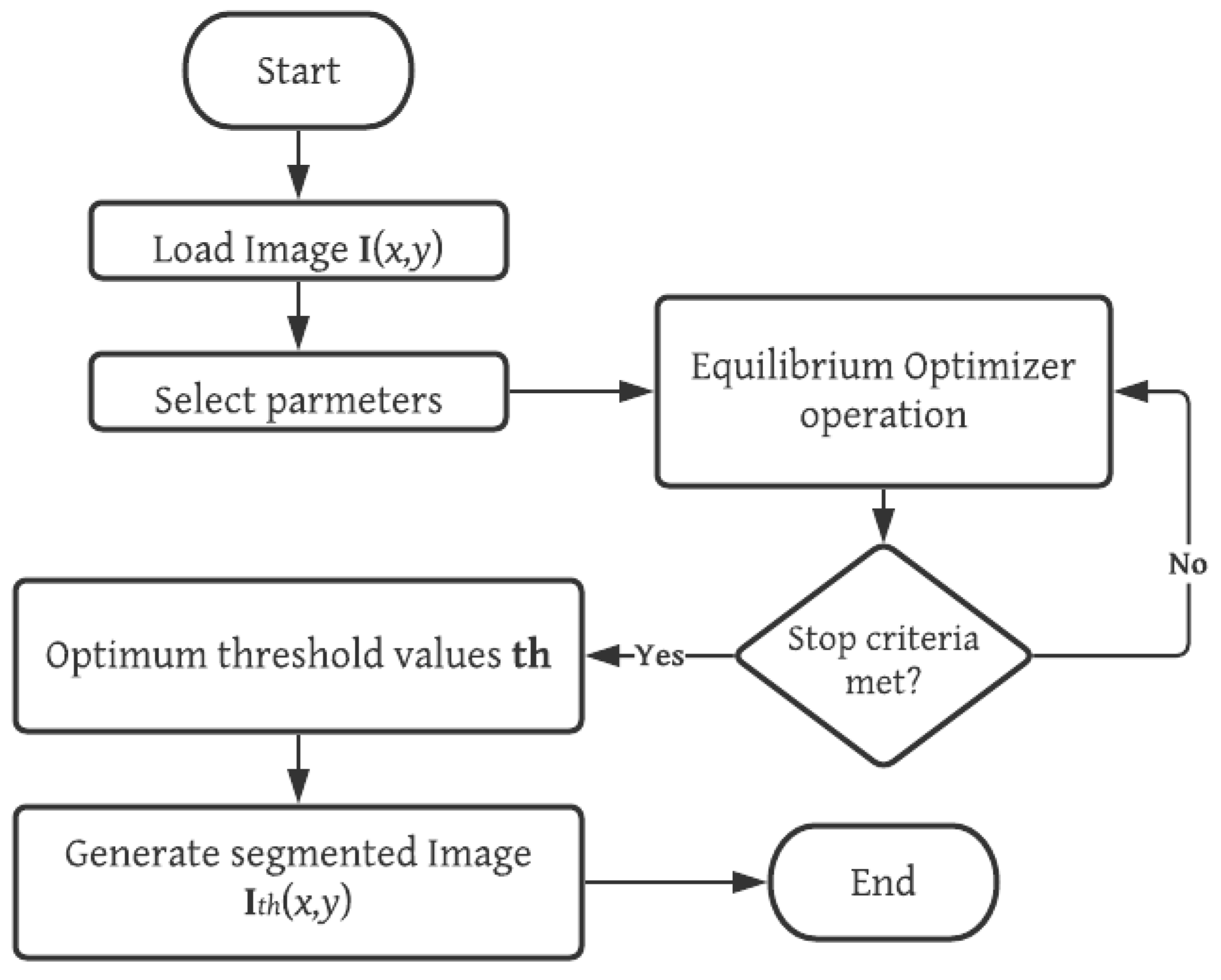
The equilibrium optimization (EO) algorithm is implemented for the solution of thresholding problems with both standard and prostate MRI images. The entire process is summarized as follows. First, the image is loaded into memory, and its grayscale histogram is computed. Then, the configuration parameters of the MCE-EO are selected. Afterwards, the iterative process of the EO is started with a randomly generated population and the solutions are iteratively enhanced through the operators of EO and the evaluation of the fitness function MCE. The MCE-EO approach stops iterating until a stop criterion is met; in this case, a fixed number of generations. Finally, the optimal set of thresholds is used to generate the segmented image. A graphical representation of the MCE-EO approach is depicted in Figure 1. The detailed implementation of MCE-EO is described in the pseudo-code of Figure 2.

Figure 1.
Overview of the proposed MCE-EO methodology for prostate MRI segmentation. This figure illustrates the stages of the multilevel cross-entropy equilibrium optimizer (MCE-EO) approach, from MRI image acquisition and preprocessing to threshold selection and segmentation. The methodology optimizes threshold values using cross-entropy, enhancing segmentation accuracy.
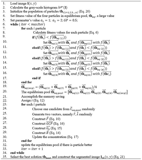
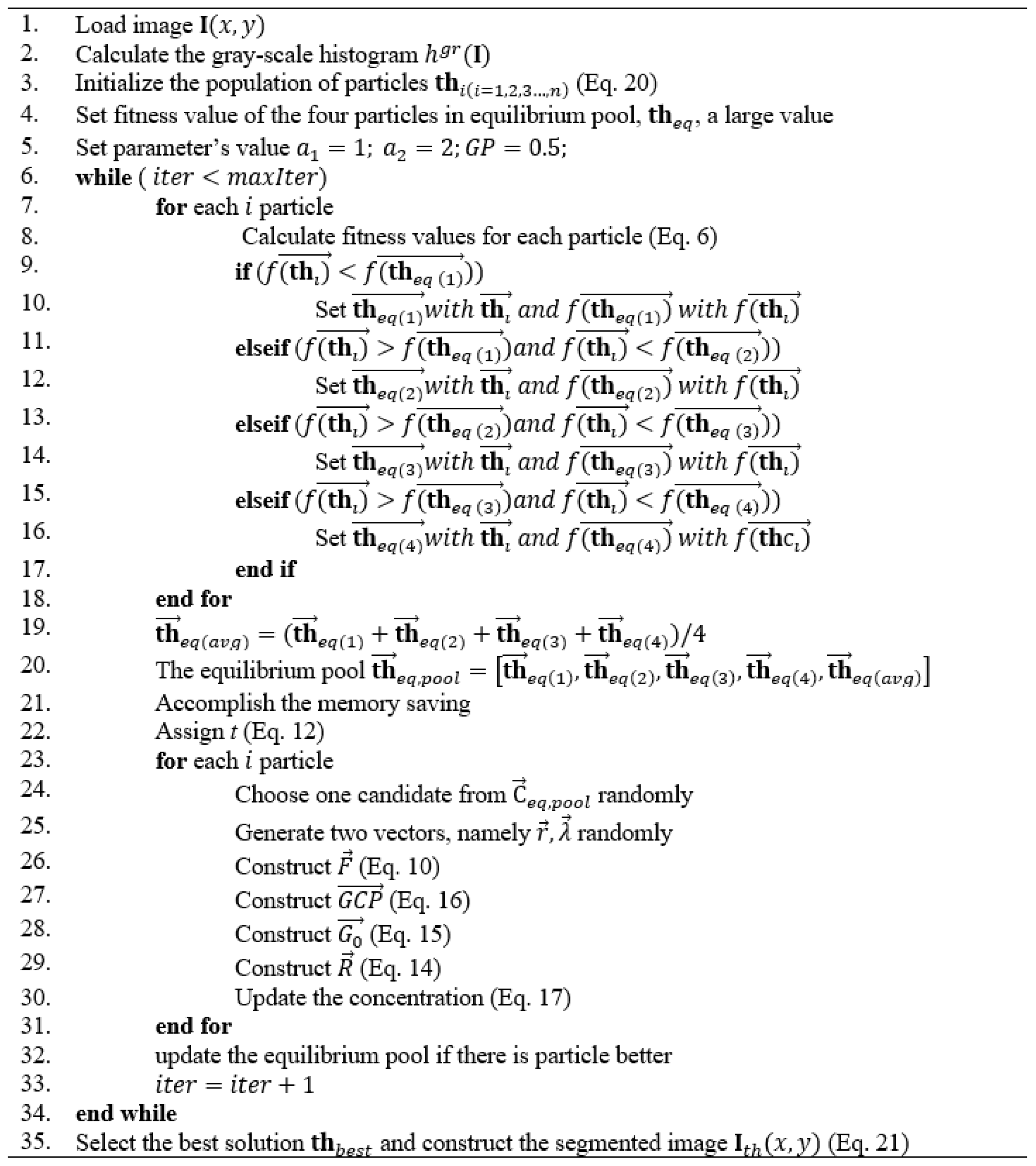
Figure 2.
Pseudocode for the implementation of the MCE-EO algorithm. This figure presents the pseudocode outlining the key steps of the MCE-EO algorithm. It includes initialization of parameters, the optimization process using the equilibrium optimizer (EO), and the evaluation of threshold values based on the minimum cross-entropy criterion. The pseudocode highlights the iterative process that leads to the selection of optimal thresholds for accurate prostate MRI segmentation.
4.5. Thresholded Image
Once the EO identifies the optimal set of threshold values for the image , it applies multilevel thresholding to generate the segmented image . The process for performing this segmentation is outlined in Equation (22). The overall MCE-EO methodology is illustrated in the flowchart shown in Figure 1.
4.6. Computational Complexity
The proposed MCE-EO uses two algorithms with different properties. First, the calculation of the minimum cross-entropy (MCE) for t thresholds is [12]. The second algorithm is the equilibrium optimizer (EO) with a reported polynomial complexity of , where c is the cost of the objective function (in this case MCE), i is the number of iterations, d indicates the dimensions, and n indicates the number of solutions at each generation [25].
5. Experiments
In this section, the proposed method is analyzed to evaluate its effectiveness over relevant images. The methodology contains two experiments. The first is designed to determine if the proposed approach is superior to related techniques over a set of eleven generally used images in the field of thresholding. After we concluded that the MCE-EO is competent for general image thresholding, we moved towards a more in-depth analysis of the performance of MCE-EO on the specific domain of prostate image segmentation with six magnetic resonance transaxial-cut prostate images. In both cases and for comparative purposes, the experiments consider six metaheuristic algorithms: the sunflower optimization (SFO) algorithm [40], the sine cosine algorithm (SCA) [41], particle swarm optimization (PSO), differential evolution (DE) [42], the genetic algorithm (GA) [43], and the Hirschberg—Sinclair algorithm (HS) [44].
In this study, all of the metaheuristic (stochastic) algorithms used the minimum cross-entropy criterion as an objective function with the same solution representation. It is important to note that the proposed thresholding-based segmentation method does not rely on ground truth data, as is often required for metrics like pixel accuracy (PA) or intersection over union (IoU). Instead, we evaluate segmentation effectiveness using no-reference image quality metrics such as peak signal-to-noise ratio (PSNR) [14], structural similarity index measure (SSIM) [46], and feature similarity index measure (FSIM) [47]. These metrics provide a robust analysis of image fidelity, structure preservation, and overall segmentation quality, which are crucial for medical imaging applications where precise anatomical boundaries are essential for diagnosis.
All experiments were performed with MATLAB R2016a using a device equipped with an 2.4 GHz Intel Core i5 CPU and 12 GB of RAM. This approach allowed us to assess the performance of the segmentation process without the need for manually annotated reference images.
5.1. Parameter Settings
Stochastic optimization algorithms (SOA) are quite sensitive to the parameter configuration of their mechanisms. The correct selection of parameters is a time-consuming task that is often avoided by using the original parameters selected by the creators of the algorithm. Most of the time, the parameters provided by the original authors are good enough for most tasks and can give us an overall idea of the performance of an algorithm on a given task. Thus, in this paper, the parameters are selected as the original authors recommended (see Table 1).

Table 1.
Parameter Settings for the algorithms. This table lists the key parameter configurations for the algorithms used in the experiments, including the equilibrium optimizer (EO) and comparison methods.
Another element having a significant impact on the performance of an algorithm is the maximum number of iterations that an algorithm is allowed to use. In this study, we have chosen 500 iterations, as we observed a convergence on most approaches prior to this limit. As their name indicates, SOAs show variability in their result. To properly compare the performance of each methodology, we used thirty runs of each experiment to generate statistically valid data.
5.2. Evaluating Image Quality
Image quality after processing can be assessed through both objective and subjective methods. Objective evaluations include numerical metrics, either with or without a reference image, where the reference is often referred to as ground truth. While having a ground truth is ideal in many cases, creating annotated datasets is time-intensive and can sometimes introduce subjectivity. To address this limitation, many methods employ no-reference quality metrics such as PSNR, SSIM, and FSIM. In MRI, a high PSNR indicates that critical anatomical details are preserved, which is crucial since noise can obscure important structures. A high SSIM value ensure that important clinical features remain intact after processing. Given the importance of features such as tissue boundaries in MRI images, a high FSIM value indicates that essential diagnostic details have been retained.
5.2.1. PSNR
The peak signal-to-noise ratio (PSNR) measures the amount of distortion noise relative to the signal power [14]. PSNR is commonly used to evaluate image quality after processing, comparing the original image with its processed (or distorted) version on a logarithmic scale. Higher PSNR values indicate better image quality. The formula to calculate PSNR is given by:
5.2.2. SSIM
The structural similarity index method (SSIM) is another no-reference quality metric, similar to PSNR, but it incorporates aspects of human visual perception. An SSIM model images distortion by assessing changes in structural information [46]. It evaluates luminance, contrast, and structural similarity, measuring the correlation between the original and processed images. The SSIM value ranges from 0 to 1, with higher values indicating better image quality. The SSIM is computed as follows:
where and are the mean value of the original and the umbralized image, respectively, and for each image, the values of and correspond to the standard deviation. and are constants used to avoid the instability when ; experimentally, in Agrawal et al. [48]), both values are C1 = C2 = 0.065.
5.2.3. FSIM
The feature similarity index method (FSIM) evaluates the quality of an image by comparing the original and processed versions based on the features present within the image. Features, such as edges and corners, are regions that contain significant information. Preserving these features during image processing is crucial for accurately interpreting the image. FSIM identifies features using two common methods: phase congruency () and gradient magnitude () [47]. The FSIM value ranges from 0 to 1, with higher values indicating better image quality. The formula for calculating FSIM is as follows:
where denotes the domain of the image
5.3. Results from Standard Test Images
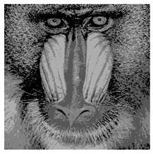
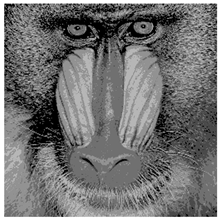
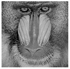
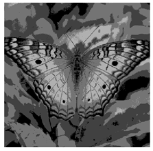
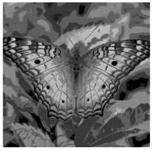
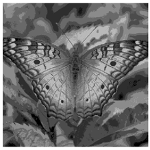
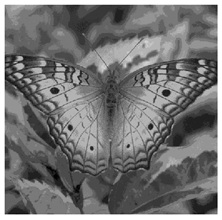
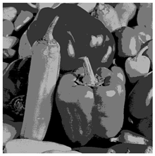
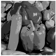
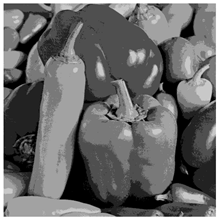
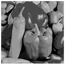
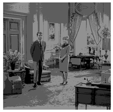
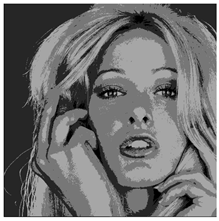
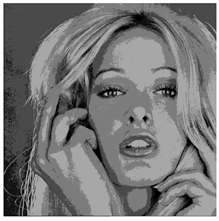
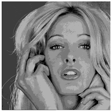
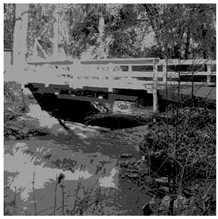
This experiment is designed to determine if the proposed approach is superior to related approaches over a set of eleven generally used images in the field of thresholding. For this purpose, we will examine the fitness and standard deviation results of the first experimental dataset, which combines eleven well-known benchmark images (Cameraman, Lenna, Baboon, Man, Jet, Peppers, Living Room, Blonde, Walk Bridge, Butterfly, and Lake).
For the experiments, the threshold levels considered for the first set of images are = 2, 3, 4, 5, and 8. The qualitative reults can be observed in Table 2.
Table 2.
Segmentation of benchmark images.
As shown in Table 3, the EO algorithm consistently outperformed the other six algorithms on average, with the performance gap becoming more apparent as the number of thresholds increased. Additionally, EO exhibited near-zero standard deviation in many tests, indicating its stability. In related studies, threshold searches have typically focused on a maximum of five levels, as increasing the number of thresholds leads to a substantial rise in computational complexity [49].
Table 3.
Fitness values of SOAs on the general-purpose image dataset. This table shows the fitness values of various stochastic optimization algorithms (SOAs) applied to the general-purpose image dataset, where lower values indicate better segmentation performance.
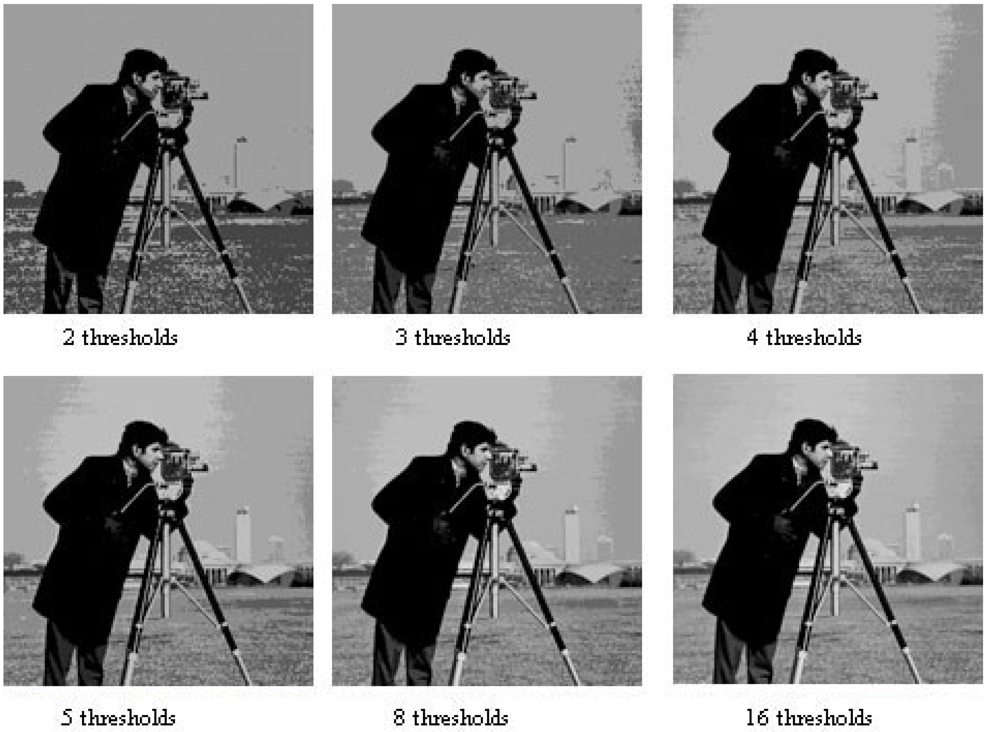
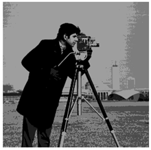
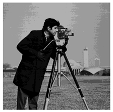
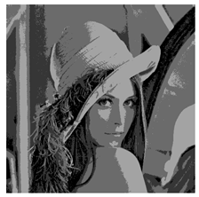
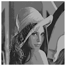
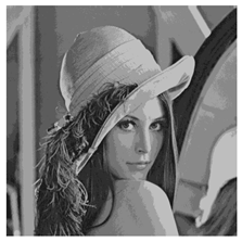
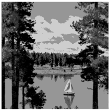
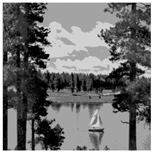
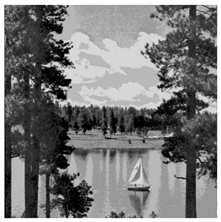
The numerical results demonstrate that EO significantly outperformed other stochastic optimization algorithms when applied to the image thresholding problem using cross-entropy. Figure 3 provides an example of a segmented image produced by the proposed method, showing the results for six different threshold levels for qualitative comparison.

Figure 3.
Cameraman image segmented with 2, 3, 4, 5, 8, and 16 thresholds. This figure displays the segmentation results of the cameraman image using different numbers of thresholds, demonstrating the progressive refinement of image regions as the number of thresholds increases.
So far, the results confirm EO’s excellent performance in image thresholding. However, since the primary focus of this work is the application of EO combined with cross-entropy for prostate MRI segmentation, the image quality analysis is presented in the second experiment.
5.4. Results from Magnetic Resonance Prostate Images
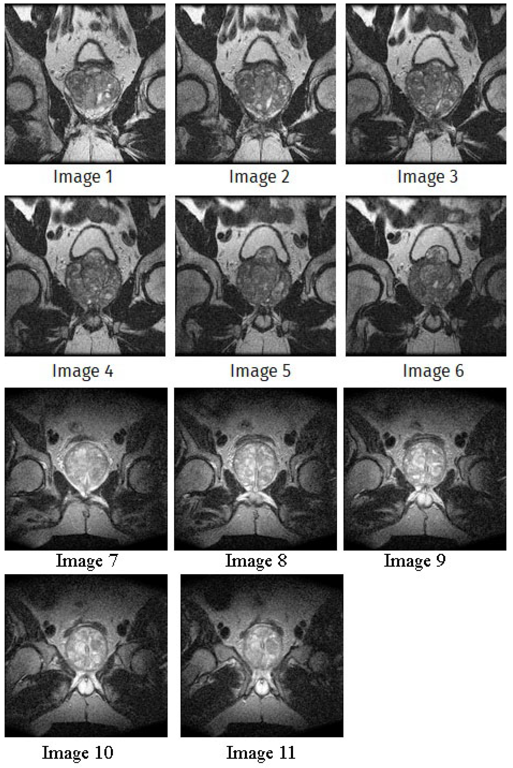
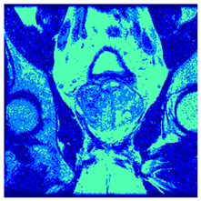
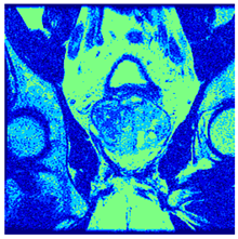
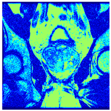
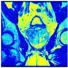
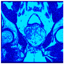
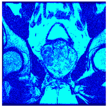
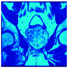
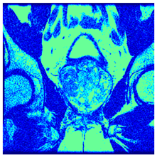
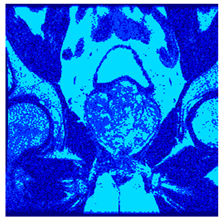
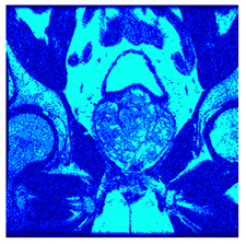
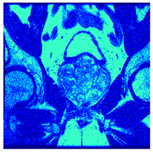
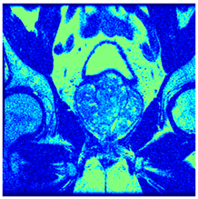
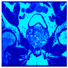
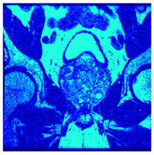
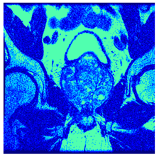
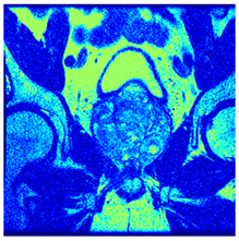
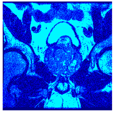
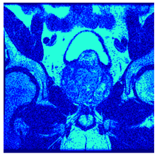
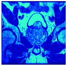
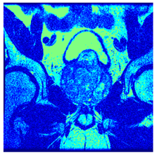
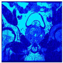
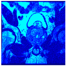
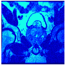
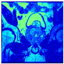
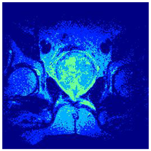
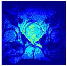
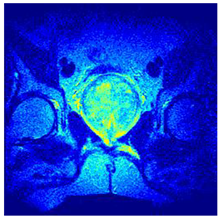
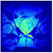
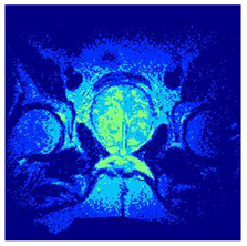
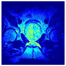
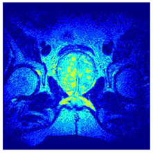
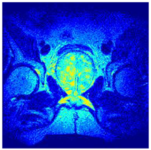
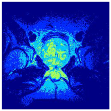
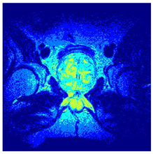
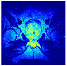
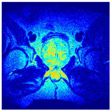
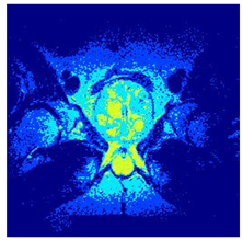
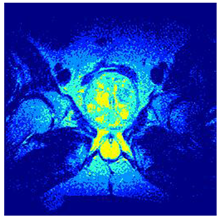
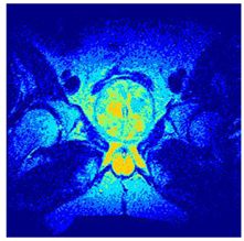
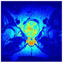
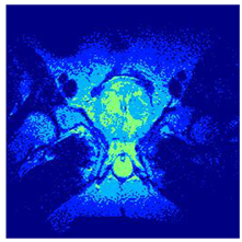
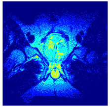
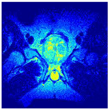
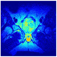
In this subsection, we will discuss the experiment designed to evaluate the performance of EO with cross-entropy for the segmentation of prostate MRI images. To this end, we use a group of reference images formed by a set of six prostate MRI images; see Figure 4. All the images from the group were extracted from the Ferenc Jolesz National Center for Image-Guided Therapy, Harvard Medical School, or Brigham Health Hospital datasets with no additional preprocessing [50]. Prostate MRI images are primarily used for disease diagnosis or to establish treatment for prostate-related diseases such as prostatitis, benign prostatic hyperplasia (BPH), and prostate cancer, among other diseases or medical conditions. In the context of this article, the images were used to test the efficiency of the equilibrium optimizing algorithm and compare it with the other six chosen algorithms. The segmentation of MRIs is carried out over four different thresholds levels: = 3, 4, 5, and 8. Due to the nature of the images, there was a limited number of different tissues in the images; thus, there was no point in evaluating a larger number of .
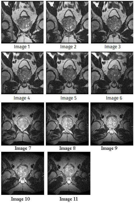
Figure 4.
Eleven transaxial-cut prostate MRI images. This figure presents a set of eleven transaxial-cut magnetic resonance (MR) images of the prostate. These images serve as the input dataset for evaluating the segmentation performance of the proposed algorithm.
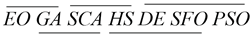
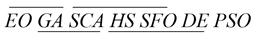
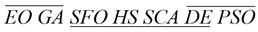
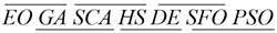
5.5. Statistical Analysis of Standard Test Images
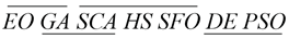
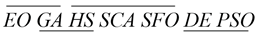
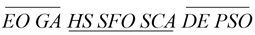
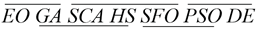
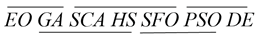
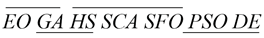
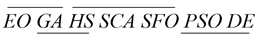
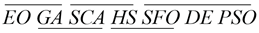
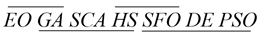
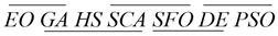
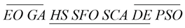
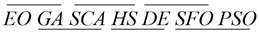
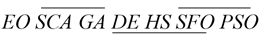
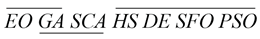
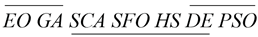
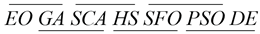
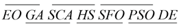
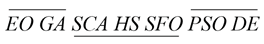
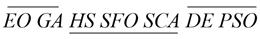
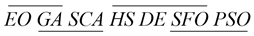
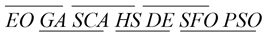
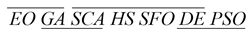
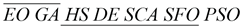
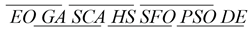
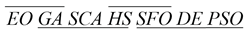
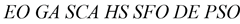
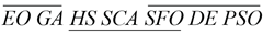
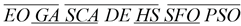
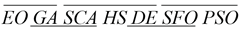
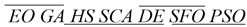
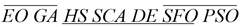
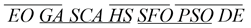
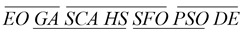
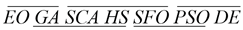
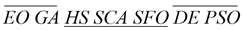
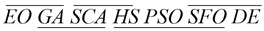
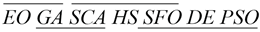
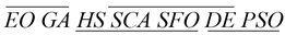
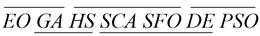
Within stochastic optimization algorithms (SOAs), it is possible that two different approaches will produce the same results. If this is true, we could say that the two methods are not statistically different. To determine if this happens and to what extent, we use the Kruskal–Wallis test, a non-parametric method that discerns if the median of two or more distributions is statistically different [51]. We could say that Kruskal–Wallis is the non-parametric counterpart of the one-way analysis of variance (ANOVA) [52]. In this article, the analysis is applied to the prostate MRIs, where each experiment considers thirty independent runs of the same configuration. Each configuration includes an algorithm and a specific number of thresholds. All statistical significance tests require the definition of a significance level to accept or reject the null hypothesis, which states that all data are coming from the same distribution. The test outputs a p-value, and if it is lower than the null hypothesis, we can be sure that the algorithms are significantly different. In Table 4, the column named Ranking indicates the rank of each method in terms of fitness; the left-most algorithm is considered the best, while the right-most is the worst. In the notation, we can observe horizontal lines originating from two or more algorithms; this indicates that such algorithms are not significantly different.
Table 4.
Mean fitness and standard deviation for magnetic resonance prostate images. This table presents the mean fitness values and standard deviations obtained from applying various algorithms to the segmentation of magnetic resonance prostate images. The results indicate the consistency and accuracy of each algorithm in optimizing the segmentation task.
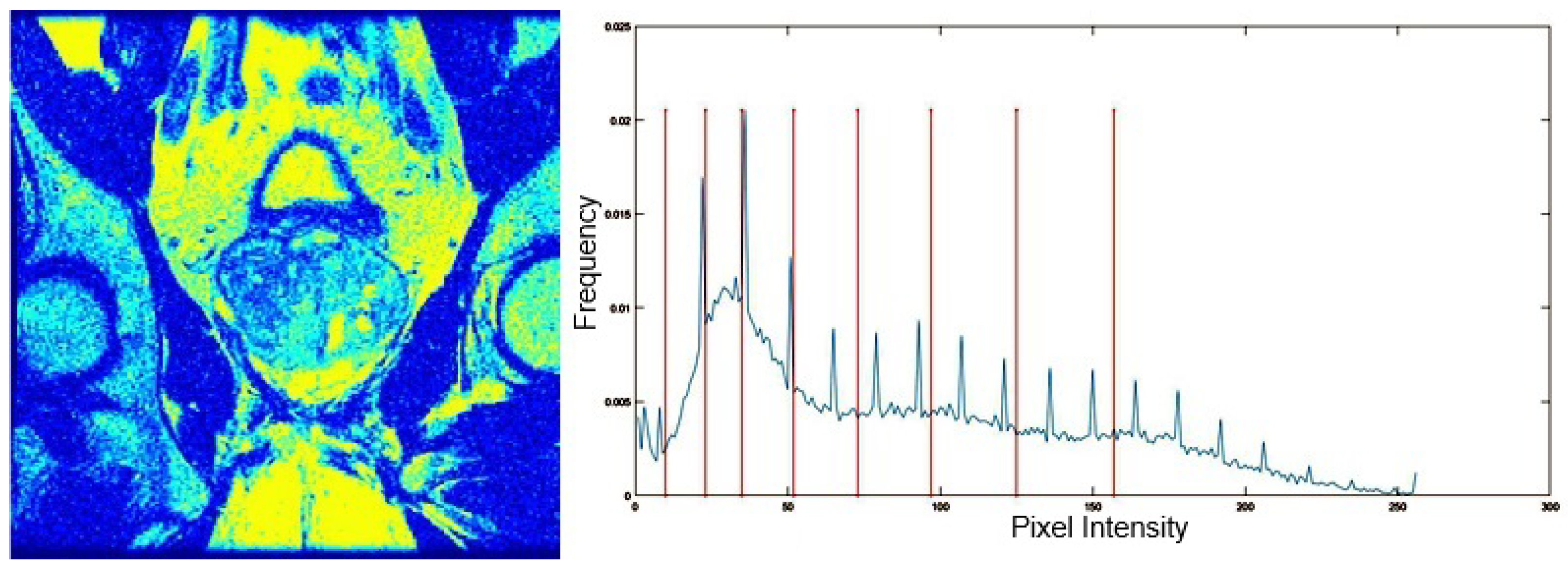
Table 5 presents the segmentation of the MRIs using EO for a qualitative inspection. From Figure 5, it is clear that two lumps in the prostate have been highlighted by the thresholding process. Prostatic MRIs present noisy conditions, which makes it difficult to visualize the thresholding with the naked eye, so in Figure 5 we present the thresholded image as well as the histogram with the values of the thresholds generated by the EO. It can be observed in the histogram that the thresholds present an adequate distribution, even though this particular image has impulsive noise and a simple shape. Our findings indicate that four thresholds are typically sufficient for this application, which corresponds to identifying five different tissue types in the image. A smaller threshold value may result in a lack of sufficient contrast to highlight relevant anatomical structures, such as the prostate capsule. In contrast, a higher number of thresholds may lead to the incorrect differentiation of anatomical regions that should be connected.
Table 5.
Segmentation of transaxial-cut prostate MRI images Using EO and cross-entropy. This table presents the segmentation results of transaxial-cut prostate MRI images using the equilibrium optimizer (EO) and cross-entropy. Each row corresponds to a distinct MRI image, while the columns nt represent the number of thresholds applied during segmentation. The results illustrate the performance of the EO algorithm across different threshold levels for each image.

Figure 5.
MRI prostatic 01 segmented with 8 thresholds and corresponding histogram. The left image shows the segmentation of the MRI prostatic 01 image using 8 thresholds. On the right, the corresponding image histogram is displayed, with vertical lines marking the selected threshold values, illustrating how the thresholds divide the intensity levels for segmentation.
5.6. Segmentation Quality
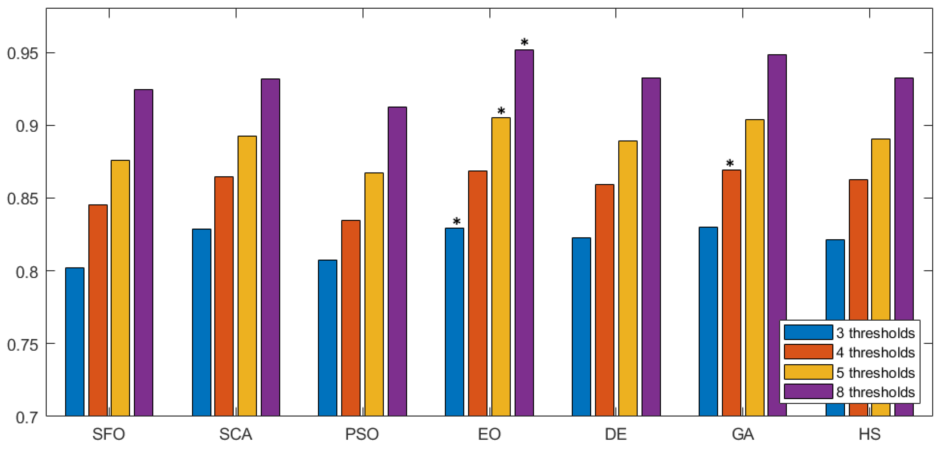
The information in Table 4 indicates that EO outperformed its counterparts in terms of the fitness function for prostate MRIs. However, the excellent performance of the algorithm over the search-space does not necessarily guarantee that it will reflect on image quality. Thus, an evaluation not associated to the fitness function is required. Here, the objective quality of the segmented image is evaluated using the three non-referenced metrics described in Section 5.3: PSNR, SSIM, and FSIM. In all metrics, a higher value points to higher-quality segmentation. Figure 6 shows a graphical comparison of the PSNR value over the different methodologies represented as seven groups along the horizontal axis. Inside each group, the average PSNR value is given for all images, considering thirty runs for a given number of thresholds (color-coded). To facilitate the interpretation of results, the best value is marked with an *. In terms of PSNR, EO outperformed the other approaches at most of threshold levels. Only GA managed to have a slightly better score on three thresholds.
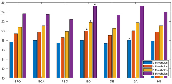
Figure 6.
PSNR comparison across methodologies. This figure shows the PSNR values of seven segmentation methods. Each group represents average PSNR values for different thresholds, with the best marked by an asterisk (*).
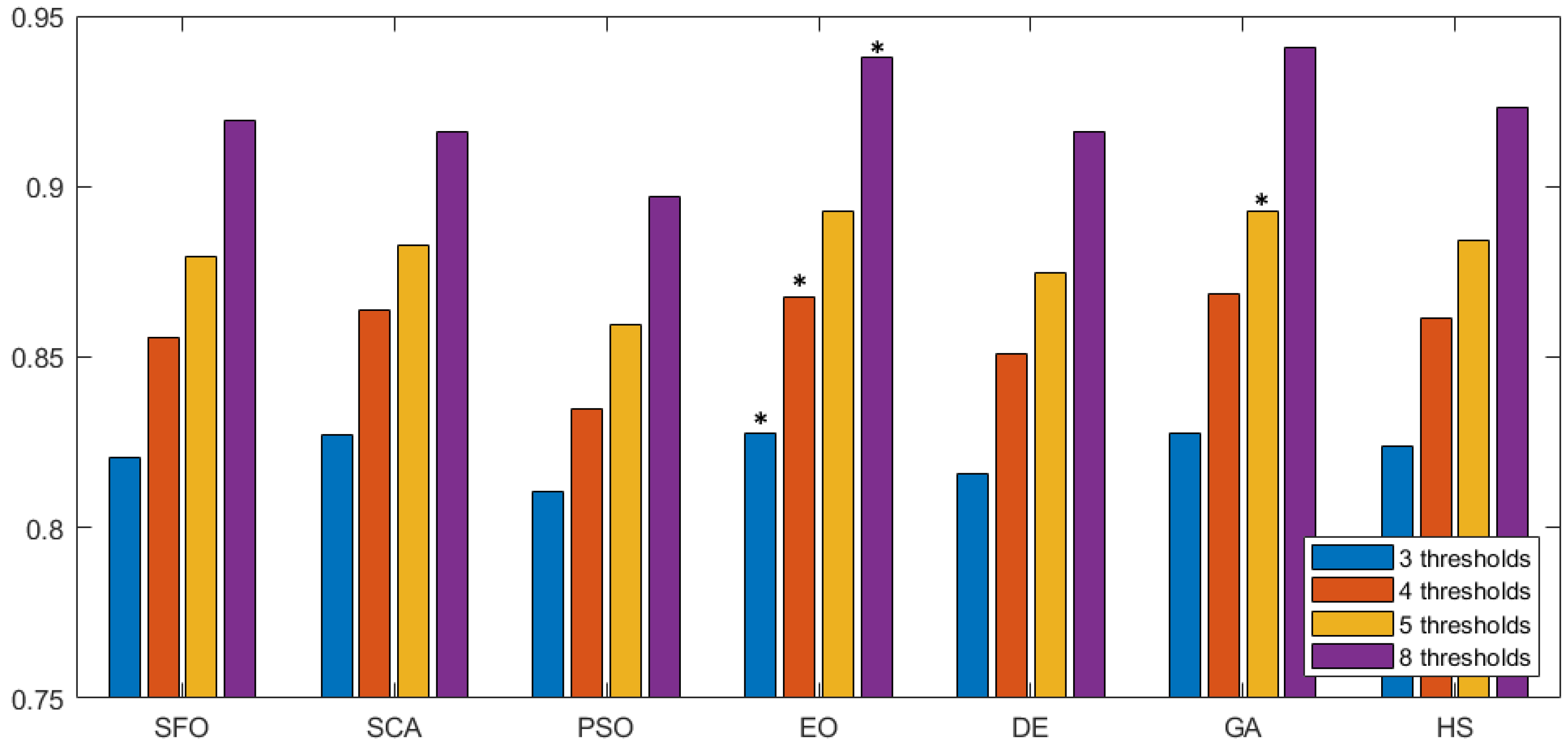
In Figure 7 we can observe the same type of graphical representation for the comparison of the SSIM value over the experiments over the horizontal axis. Each group takes the average SSIM value for all images for a given number of thresholds. In this case, the GA algorithm was able to outperform over five thresholds. In the rest of the experiments, EO consistently performed better than the other approaches. Following the same representation, the FSIM is analyzed in Figure 8, where GA has a marginal victory with five thresholds, while EO scores better in the other cases. In summary, we can observe that PSNR, SSIM, and FSIM objectively indicate that EO is better than the other approaches for the segmentation of prostate MRIs.
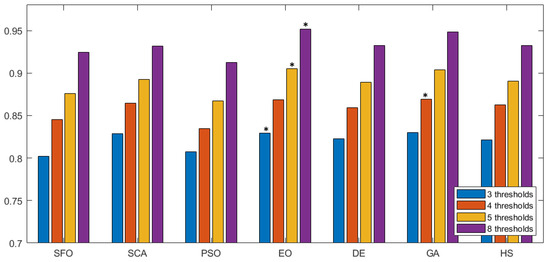
Figure 7.
Comparative study of SSIM across different methodologies. This figure presents a comparison of SSIM values for various segmentation methodologies. Each group along the horizontal axis represents different methods, with SSIM values evaluated over multiple thresholds. The results highlight the structural similarity performance of each approach, with higher SSIM values indicating better preservation of image structure during segmentation. The the best is marked by an asterisk (*).

Figure 8.
FSIM comparison across methodologies. This figure compares FSIM values for different segmentation methods, with each group representing a method and various threshold settings. Higher FSIM values indicate better feature preservation during segmentation. The the best is marked by an asterisk (*).
6. Conclusions and Future Work
This paper introduces a novel approach, MCE-EO, designed to determine an optimal set of threshold values for effectively segmenting prostate MRI images. The method is based on the equilibrium optimizer (EO), a stochastic optimization algorithm, and employs minimum cross-entropy as a non-parametric criterion. The efficacy of MCE-EO is assessed through two experiments. The first experiment evaluates the performance of EO in segmenting general-purpose images, while the second focuses on prostate MRI segmentation. In both cases, MCE-EO is compared against several other stochastic optimization algorithms, including the sunflower optimization (SFO) algorithm, sine cosine algorithm (SCA), particle swarm optimization (PSO), differential evolution (DE), the genetic algorithm (GA), and the Hirschberg–Sinclair algorithm (HS). Additionally, statistical significance was assessed using a post-hoc test. The segmentation quality for MRI images was evaluated using key objective quality metrics such as peak signal-to-noise ratio (PSNR), structural similarity index Measure (SSIM), and feature similarity index (FSIM).
In conclusion, the proposed MCE-EO method for prostate MRI segmentation outperformed several other metaheuristic algorithms, including SFO, SCA, and PSO. In experiments involving standard datasets and transaxial-cut prostate MRIs, MCE-EO achieved superior segmentation accuracy, with higher values of PSNR, SSIM, and FSIM, demonstrating its robustness and effectiveness in handling complex medical images. These results confirm the potential of MCE-EO in improving the early detection of prostate cancer, where accurate image segmentation is critical for diagnosis and treatment planning.
Future Work
The combination of the equilibrium optimizer (EO) and minimum cross-entropy (MCE) has demonstrated favorable outcomes for prostate MRI segmentation. However, there are a few limitations that require attention. A significant challenge is the computational time required by EO, particularly when working with large datasets or high-resolution MRI scans. While the iterative nature of the process is an effective approach, it can result in slower processing times, which may be a disadvantage in clinical settings where rapid analysis is essential. Further research could concentrate on optimizing EO through parallel computing, hybrid algorithms, or reducing the number of iterations without affecting accuracy.
A further limitation results from the the variability in segmentation quality across different imaging types. EO performs well in prostate MRI, but may require adjustments for other modalities, such as ultrasound or CT scans. Further work could investigate the potential of adapting EO to a range of imaging techniques by incorporating mechanisms that tailor the algorithm to the specific characteristics of each modality.
Author Contributions
Conceptualization, O.Z. and S.H.; methodology, O.Z. and D.O.-J.; software, D.O.-J.; writing—original draft preparation, O.Z. and S.H. All authors have read and agreed to the published version of the manuscript.
Funding
This research received no external funding.
Data Availability Statement
The results generated during the current study are available from the corresponding author on reasonable request.
Conflicts of Interest
The authors declare no conflicts of interest.
References
- Krupa, K.; Bekiesińska-Figatowska, M. Artifacts in Magnetic Resonance Imaging. Pol. J. Radiol. 2015, 80, 93–106. [Google Scholar] [CrossRef] [PubMed]
- Ghose, S.; Oliver, A.; Martí, R.; Lladó, X.; Vilanova, J.C.; Freixenet, J.; Mitra, J.; Sidibé, D.; Meriaudeau, F. A survey of prostate segmentation methodologies in ultrasound, magnetic resonance and computed tomography images. Comput. Methods Programs Biomed. 2012, 108, 262–287. [Google Scholar] [CrossRef] [PubMed]
- Bray, F.; Laversanne, M.; Sung, H.; Ferlay, J.; Siegel, R.L.; Soerjomataram, I.; Jemal, A. Global cancer statistics 2022: GLOBOCAN estimates of incidence and mortality worldwide for 36 cancers in 185 countries. CA Cancer J. Clin. 2024, 74, 229–263. [Google Scholar] [CrossRef]
- Juneja, M.; Saini, S.K.; Gupta, J.; Garg, P.; Thakur, N.; Sharma, A.; Mehta, M.; Jindal, P. Survey of denoising, segmentation and classification of magnetic resonance imaging for prostate cancer. Multimed. Tools Appl. 2021, 80, 29199–29249. [Google Scholar] [CrossRef]
- Wang, G.; Li, Z.; Weng, G.; Chen, Y. An optimized denoised bias correction model with local pre-fitting function for weak boundary image segmentation. Signal Process. 2024, 220, 109448. [Google Scholar] [CrossRef]
- Otsu, N. A threshold selection method from gray-level histograms. IEEE Trans. Syst. Man Cybern. 1979, 9, 62–66. [Google Scholar] [CrossRef]
- Menendez, M. Shannon’s entropy in exponential families: Statistical applications. Appl. Math. Lett. 2000, 13, 37–42. [Google Scholar] [CrossRef]
- Kapur, J.N.; Sahoo, P.K.; Wong, A.K. A new method for gray-level picture thresholding using the entropy of the histogram. Comput. Vis. Graph. Image Process. 1985, 29, 273–285. [Google Scholar] [CrossRef]
- Tsallis, C. Computational applications of nonextensive statistical mechanics. J. Comput. Appl. Math. 2009, 227, 51–58. [Google Scholar] [CrossRef]
- Beadle, E.; Schroeder, J.; Moran, B.; Suvorova, S. An overview of Renyi Entropy and some potential applications. In Proceedings of the 2008 42nd Asilomar Conference on Signals, Systems and Computers, Pacific Grove, CA, USA, 26–29 October 2008; pp. 1698–1704. [Google Scholar]
- Li, C.H.; Lee, C. Minimum cross entropy thresholding. Pattern Recognit. 1993, 26, 617–625. [Google Scholar] [CrossRef]
- Tang, K.; Yuan, X.; Sun, T.; Yang, J.; Gao, S. An improved scheme for minimum cross entropy threshold selection based on genetic algorithm. Knowl.-Based Syst. 2011, 24, 1131–1138. [Google Scholar] [CrossRef]
- Kennedy, J.; Eberhart, R. Particle swarm optimization. In Proceedings of the ICNN’95-International Conference on Neural Networks, Perth, Australia, 27 November–1 December 1995; Volume 4, pp. 1942–1948. [Google Scholar]
- Avcibas, I.; Sankur, B.; Sayood, K. Statistical evaluation of image quality measures. J. Electron. Imaging 2002, 11, 206–223. [Google Scholar]
- Mirjalili, S.; Mirjalili, S.M.; Lewis, A. Grey wolf optimizer. Adv. Eng. Softw. 2014, 69, 46–61. [Google Scholar] [CrossRef]
- Liu, Y.; Mu, C.; Kou, W.; Liu, J. Modified particle swarm optimization-based multilevel thresholding for image segmentation. Soft Comput. 2015, 19, 1311–1327. [Google Scholar] [CrossRef]
- Khairuzzaman, A.K.M.; Chaudhury, S. Multilevel thresholding using grey wolf optimizer for image segmentation. Expert Syst. Appl. 2017, 86, 64–76. [Google Scholar] [CrossRef]
- Miller, B.L.; Goldberg, D.E. Genetic algorithms, selection schemes, and the varying effects of noise. Evol. Comput. 1996, 4, 113–131. [Google Scholar] [CrossRef]
- Naik, M.K.; Panda, R.; Abraham, A. An entropy minimization based multilevel colour thresholding technique for analysis of breast thermograms using equilibrium slime mould algorithm. Appl. Soft Comput. 2021, 113, 107955. [Google Scholar] [CrossRef]
- Houssein, E.H.; Emam, M.M.; Ali, A.A. Improved manta ray foraging optimization for multi-level thresholding using COVID-19 CT images. Neural Comput. Appl. 2021, 33, 16899–16919. [Google Scholar] [CrossRef]
- Avalos, O.; Ayala, E.; Wario, F.; Pérez-Cisneros, M. An accurate Cluster chaotic optimization approach for digital medical image segmentation. Neural Comput. Appl. 2021, 33, 10057–10091. [Google Scholar] [CrossRef]
- Panda, R.; Samantaray, L.; Das, A.; Agrawal, S.; Abraham, A. A novel evolutionary row class entropy based optimal multi-level thresholding technique for brain MR images. Expert Syst. Appl. 2021, 168, 114426. [Google Scholar] [CrossRef]
- Houssein, E.H.; Emam, M.M.; Ali, A.A. An efficient multilevel thresholding segmentation method for thermography breast cancer imaging based on improved chimp optimization algorithm. Expert Syst. Appl. 2021, 185, 115651. [Google Scholar] [CrossRef]
- Wolpert, D.H.; Macready, W.G. No free lunch theorems for optimization. IEEE Trans. Evol. Comput. 1997, 1, 67–82. [Google Scholar] [CrossRef]
- Faramarzi, A.; Heidarinejad, M.; Stephens, B.; Mirjalili, S. Equilibrium optimizer: A novel optimization algorithm. Knowl.-Based Syst. 2020, 191, 105190. [Google Scholar] [CrossRef]
- Abdul-hamied, D.T.; Shaheen, A.M.; Salem, W.A.; Gabr, W.I.; El-sehiemy, R.A. Equilibrium optimizer based multi dimensions operation of hybrid AC/DC grids. Alex. Eng. J. 2020, 59, 4787–4803. [Google Scholar] [CrossRef]
- Menesy, A.S.; Sultan, H.M.; Kamel, S. Extracting model parameters of proton exchange membrane fuel cell using equilibrium optimizer algorithm. In Proceedings of the 2020 International Youth Conference on Radio Electronics, Electrical and Power Engineering (REEPE), Moscow, Russia, 12–14 March 2020; pp. 1–7. [Google Scholar]
- Rabehi, A.; Nail, B.; Helal, H.; Douara, A.; Ziane, A.; Amrani, M.; Akkal, B.; Benamara, Z. Optimal estimation of Schottky diode parameters using a novel optimization algorithm: Equilibrium optimizer. Superlattices Microstruct. 2020, 146, 106665. [Google Scholar] [CrossRef]
- Abdel-Basset, M.; Mohamed, R.; Mirjalili, S.; Chakrabortty, R.K.; Ryan, M.J. Solar photovoltaic parameter estimation using an improved equilibrium optimizer. Sol. Energy 2020, 209, 694–708. [Google Scholar] [CrossRef]
- Yıldız, A.R.; Özkaya, H.; Yıldız, M.; Bureerat, S.; Yıldız, B.; Sait, S.M. The equilibrium optimization algorithm and the response surface-based metamodel for optimal structural design of vehicle components. Mater. Test. 2020, 62, 492–496. [Google Scholar] [CrossRef]
- Elsheikh, A.H.; Shehabeldeen, T.A.; Zhou, J.; Showaib, E.; Abd Elaziz, M. Prediction of laser cutting parameters for polymethylmethacrylate sheets using random vector functional link network integrated with equilibrium optimizer. J. Intell. Manuf. 2021, 32, 1377–1388. [Google Scholar] [CrossRef]
- Nguyen, T.; Nguyen, G.; Nguyen, B.M. EO-CNN: An enhanced CNN model trained by equilibrium optimization for traffic transportation prediction. Procedia Comput. Sci. 2020, 176, 800–809. [Google Scholar] [CrossRef]
- Gao, Y.; Zhou, Y.; Luo, Q. An efficient binary equilibrium optimizer algorithm for feature selection. IEEE Access 2020, 8, 140936–140963. [Google Scholar] [CrossRef]
- Zheng-Ming, G.; Juan, Z.; Su-Ruo, L.; Ru-Rong, H. The improved Equilibrium Optimization Algorithm with Tent Map. In Proceedings of the 2020 5th International Conference on Computer and Communication Systems (ICCCS), Shanghai, China, 15–18 May 2020; pp. 343–346. [Google Scholar]
- Zhao, J.; Gao, Z. The Improved Equilibrium Optimization Algorithm with Best Candidates. J. Phys. Conf. Ser. 2020, 1575, 012089. [Google Scholar] [CrossRef]
- Gupta, S.; Deep, K.; Mirjalili, S. An efficient equilibrium optimizer with mutation strategy for numerical optimization. Appl. Soft Comput. 2020, 96, 106542. [Google Scholar] [CrossRef]
- Abdel-Basset, M.; Mohamed, R.; Abouhawwash, M. Balanced multi-objective optimization algorithm using improvement based reference points approach. Swarm Evol. Comput. 2021, 60, 100791. [Google Scholar] [CrossRef]
- Abdel-Basset, M.; Chang, V.; Mohamed, R. A novel equilibrium optimization algorithm for multi-thresholding image segmentation problems. Neural Comput. Appl. 2021, 33, 10685–10718. [Google Scholar] [CrossRef]
- Wunnava, A.; Naik, M.K.; Panda, R.; Jena, B.; Abraham, A. A novel interdependence based multilevel thresholding technique using adaptive equilibrium optimizer. Eng. Appl. Artif. Intell. 2020, 94, 103836. [Google Scholar] [CrossRef]
- Gomes, G.F.; da Cunha, S.S.; Ancelotti, A.C. A sunflower optimization (SFO) algorithm applied to damage identification on laminated composite plates. Eng. Comput. 2019, 35, 619–626. [Google Scholar] [CrossRef]
- Mirjalili, S. SCA: A sine cosine algorithm for solving optimization problems. Knowl.-Based Syst. 2016, 96, 120–133. [Google Scholar] [CrossRef]
- Storn, R.; Price, K. Differential evolution–a simple and efficient heuristic for global optimization over continuous spaces. J. Glob. Optim. 1997, 11, 341–359. [Google Scholar] [CrossRef]
- Goldberg, D.E.; Holland, J.H. Genetic algorithms and machine learning. Mach. Learn. 1988, 3, 95–99. [Google Scholar] [CrossRef]
- Peterson, G.L. An O (n log n) unidirectional algorithm for the circular extrema problem. ACM Trans. Program. Lang. Syst. (TOPLAS) 1982, 4, 758–762. [Google Scholar] [CrossRef]
- Kullback, S. Information Theory and Statistics; Courier Corporation: North Chelmsford, MA, USA, 1997. [Google Scholar]
- Wang, Z.; Bovik, A.C.; Sheikh, H.R.; Simoncelli, E.P. Image quality assessment: From error visibility to structural similarity. IEEE Trans. Image Process. 2004, 13, 600–612. [Google Scholar] [CrossRef] [PubMed]
- Zhang, L.; Zhang, L.; Mou, X.; Zhang, D. FSIM: A feature similarity index for image quality assessment. IEEE Trans. Image Process. 2011, 20, 2378–2386. [Google Scholar] [CrossRef] [PubMed]
- Agrawal, S.; Panda, R.; Bhuyan, S.; Panigrahi, B.K. Tsallis entropy based optimal multilevel thresholding using cuckoo search algorithm. Swarm Evol. Comput. 2013, 11, 16–30. [Google Scholar] [CrossRef]
- Rodriguez-Esparza, E.; Zanella-Calzada, L.A.; Oliva, D.; Heidari, A.A.; Zaldivar, D.; Pérez-Cisneros, M.; Foong, L.K. An efficient Harris hawks-inspired image segmentation method. Expert Syst. Appl. 2020, 155, 113428. [Google Scholar] [CrossRef]
- The Ferenc Jolesz National Center for Image Guided Therapy, Harvard Medical School, B.H.H. Prostate MR Image Database. Available online: https://prostatemrimagedatabase.com/index.html (accessed on 15 March 2023).
- Theodorsson-Norheim, E. Kruskal-Wallis test: BASIC computer program to perform nonparametric one-way analysis of variance and multiple comparisons on ranks of several independent samples. Comput. Methods Programs Biomed. 1986, 23, 57–62. [Google Scholar] [CrossRef]
- Scheffe, H. The Analysis of Variance; John Wiley & Sons: Hoboken, NJ, USA, 1999; Volume 72. [Google Scholar]


Disclaimer/Publisher’s Note: The statements, opinions and data contained in all publications are solely those of the individual author(s) and contributor(s) and not of MDPI and/or the editor(s). MDPI and/or the editor(s) disclaim responsibility for any injury to people or property resulting from any ideas, methods, instructions or products referred to in the content. |
© 2024 by the authors. Licensee MDPI, Basel, Switzerland. This article is an open access article distributed under the terms and conditions of the Creative Commons Attribution (CC BY) license (https://creativecommons.org/licenses/by/4.0/).