5.1. Performance Analysis
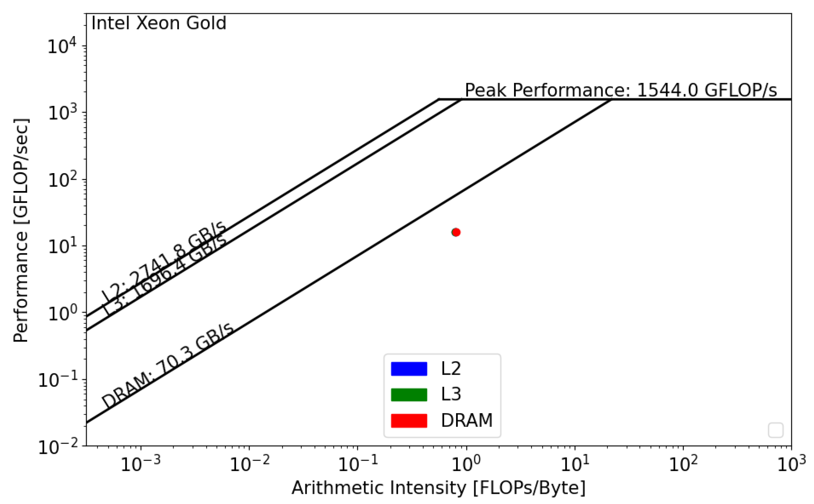
The CPU roofline models are presented below. We used dataset . The main difference between the two CPUs is the DRAM bandwidth. For the Intel Xeon processor, the memory bandwidth is equal to 70.3 GB/s, and, for the AMD EPYC processor, it is equal to 221.1 GB/s. Regarding the Floating Point performance, Intel Xeon has the lead with a = 1544 GFLOP/s. However, since the GRICS reconstruction relies on repeated FFT, the code will likely be impacted by the memory bandwidth, and efforts should be undertaken in this direction to optimize the code.
Intel SDE and Vtune report that the GRICS’s operational intensity
is equal to
FLOP/byte. AMD
Prof reports that
FLOP/byte. Using
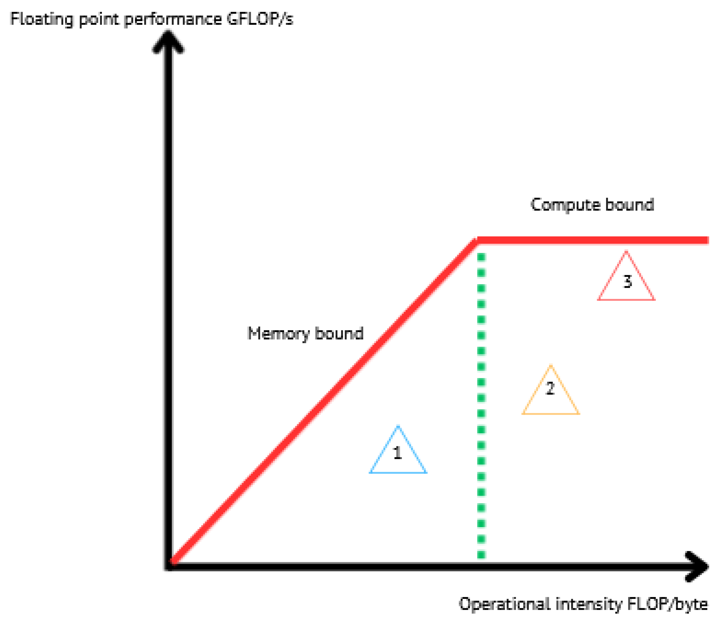
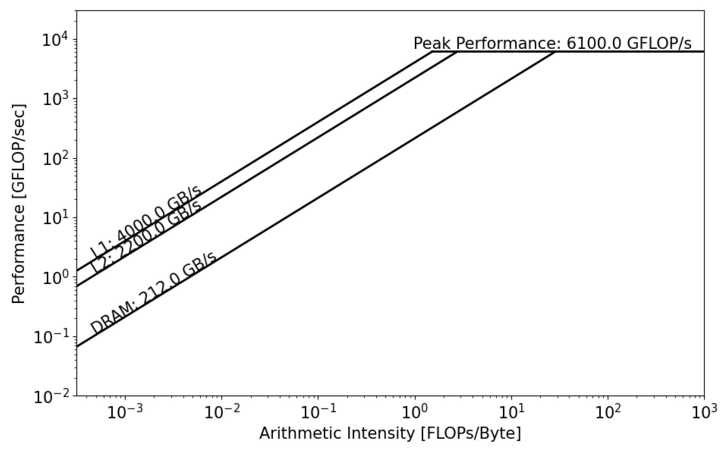
Figure 8 and
Figure 9, we can see that, in both architectures, the GRICS is memory bound. In Intel Xeon, the code is mainly limited by the low value of the DRAM bandwidth; its actual performance
is equal to 16 GFLOP/s.
is far from the theoretical bound for this value of operational intensity; a code that has a similar value of
and that uses the micro-architecture of the processor in a better way can operate at a performance
equal to 56 GFLOP/s. Using Equation (4), the code’s architectural efficiency on Xeon is 28%. On the AMD EPYC CPU, it performs better, with a performance
equal to 80 GFLOP/s. In this architecture, the code benefits from the high value of the memory bandwidth,
GB/s. Its architectural efficiency on EPYC is 52%. Moreover, the figures show that
, which means that there is poor data reuse; once the data are loaded from the main memory, they are not reused while being in caches and instead evicted. This is not the case regarding the AMD EPYC CPU, where
is greater than
and
, which means that the data are being reused once they are loaded from DRAM.
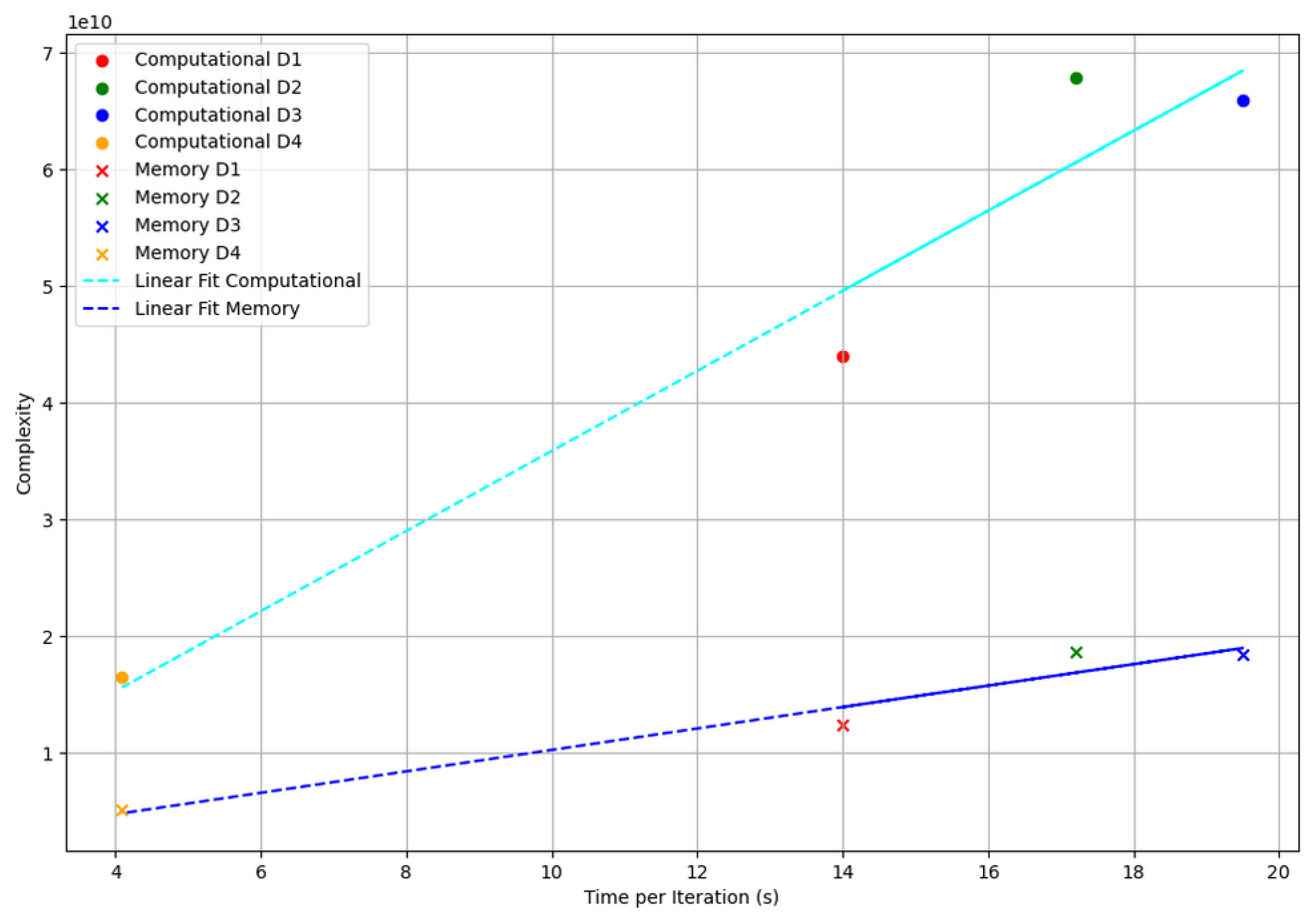
Figure 10 presents the computational and memory complexity of Algorithm 2 as a function of the elapsed time per iteration on the AMD EPYC CPU. The complexities are computed using Equations (7) and (8). Datasets
and
align closely with the predicted trend, both for memory and computation.
lies above the linear fitting lines, suggesting lower computational and memory efficiency than expected.
shows both good memory and computational efficiency, positioned below the fitting lines.
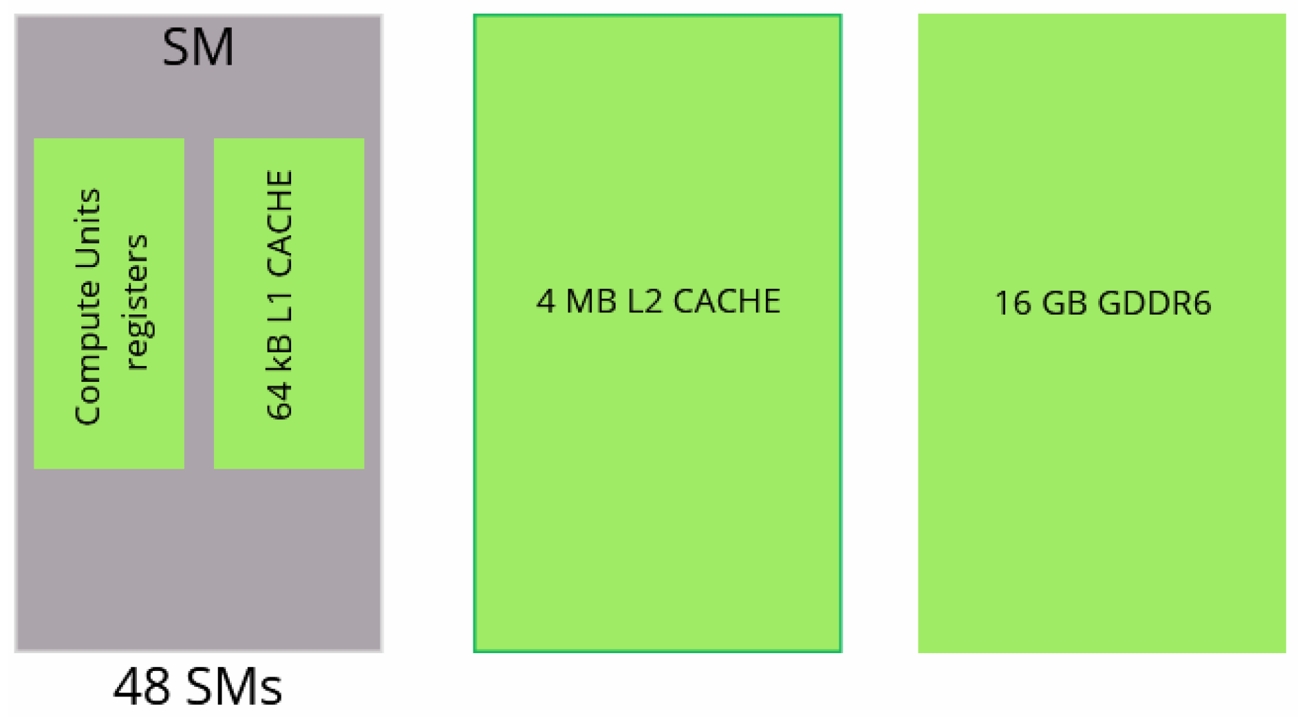
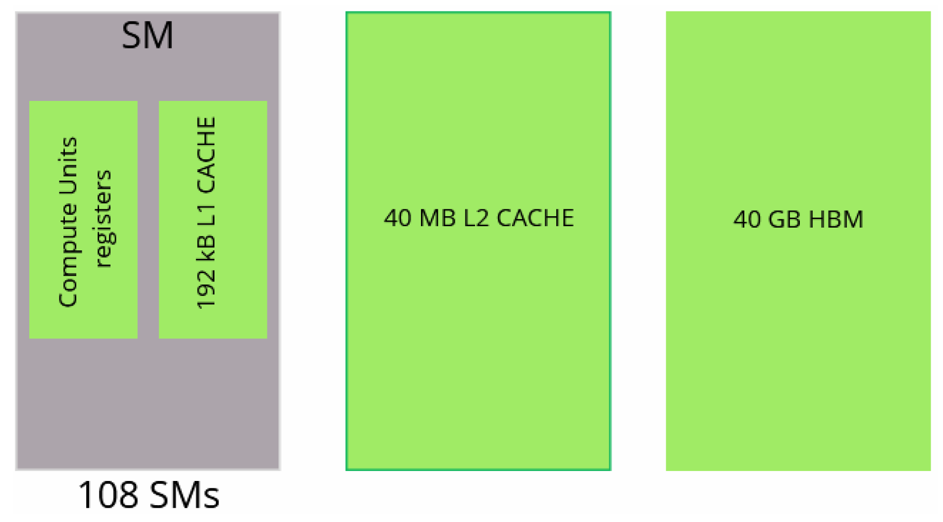
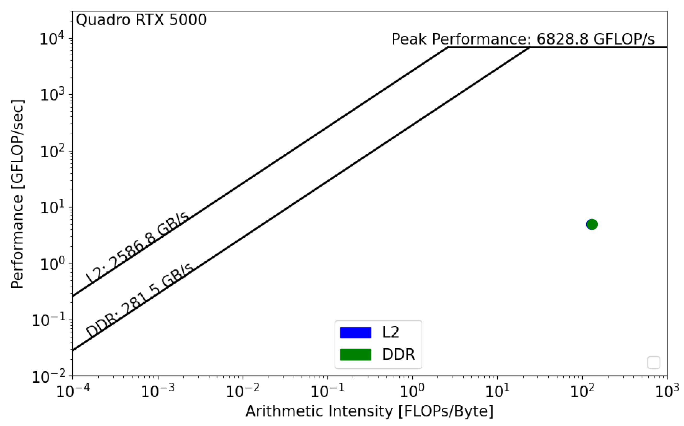
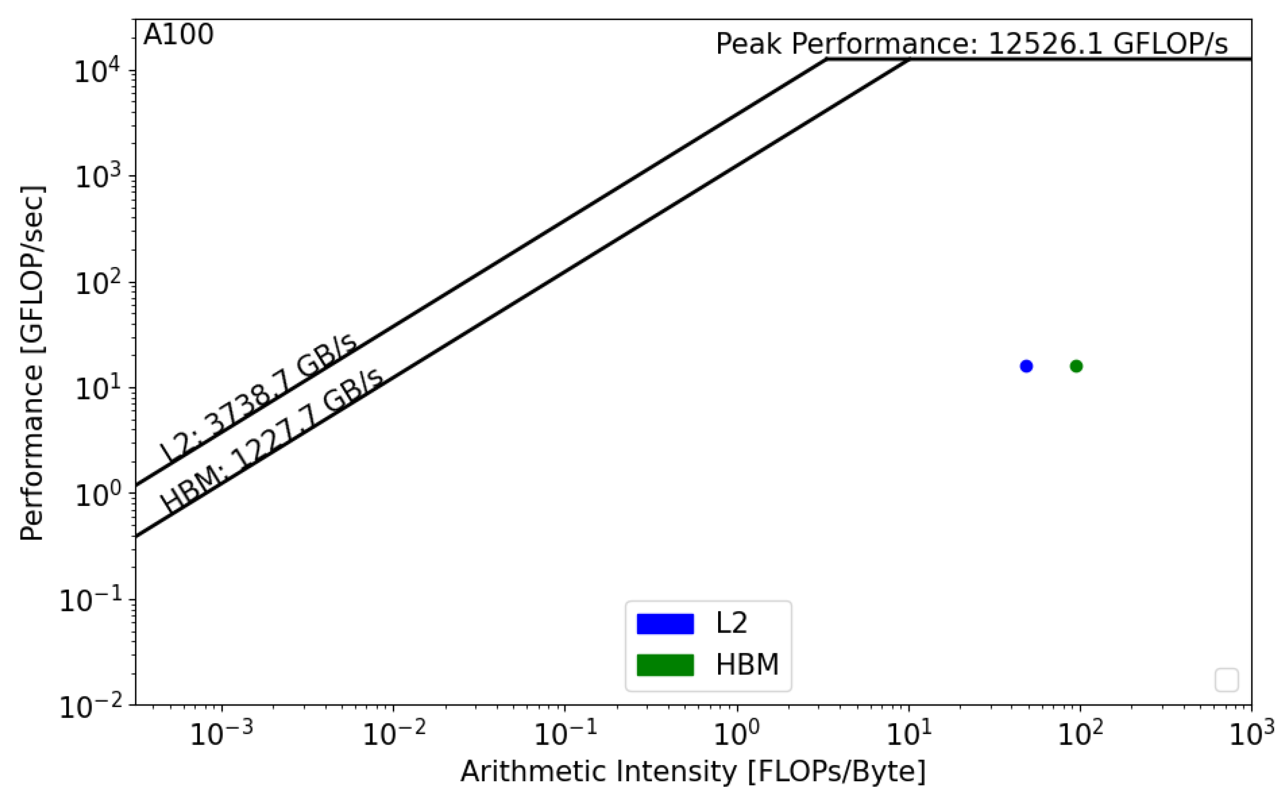
Figure 11 and
Figure 12 present the GPU roofline models. In both architectures, the reconstruction kernel is compute bound. The kernel’s performance on RTX 5000
is equal to 5 GFLOP/s, while its performance on A100,
, is equal to 16 GFLOP/s. In both cases, the actual performance is far from the roofline boundaries, which means that the actual implementation does not properly use the GPU architecture and that source-code modifications should be considered in order to achieve better performance. Moreover, we notice the absence of data reuse on Quadro RTX,
, which means that there are repetitive calls to the main memory in order to satisfy the load and store operations. However, the data are being reused on A100, which reduces the latency and improves the overall performance of the kernel.
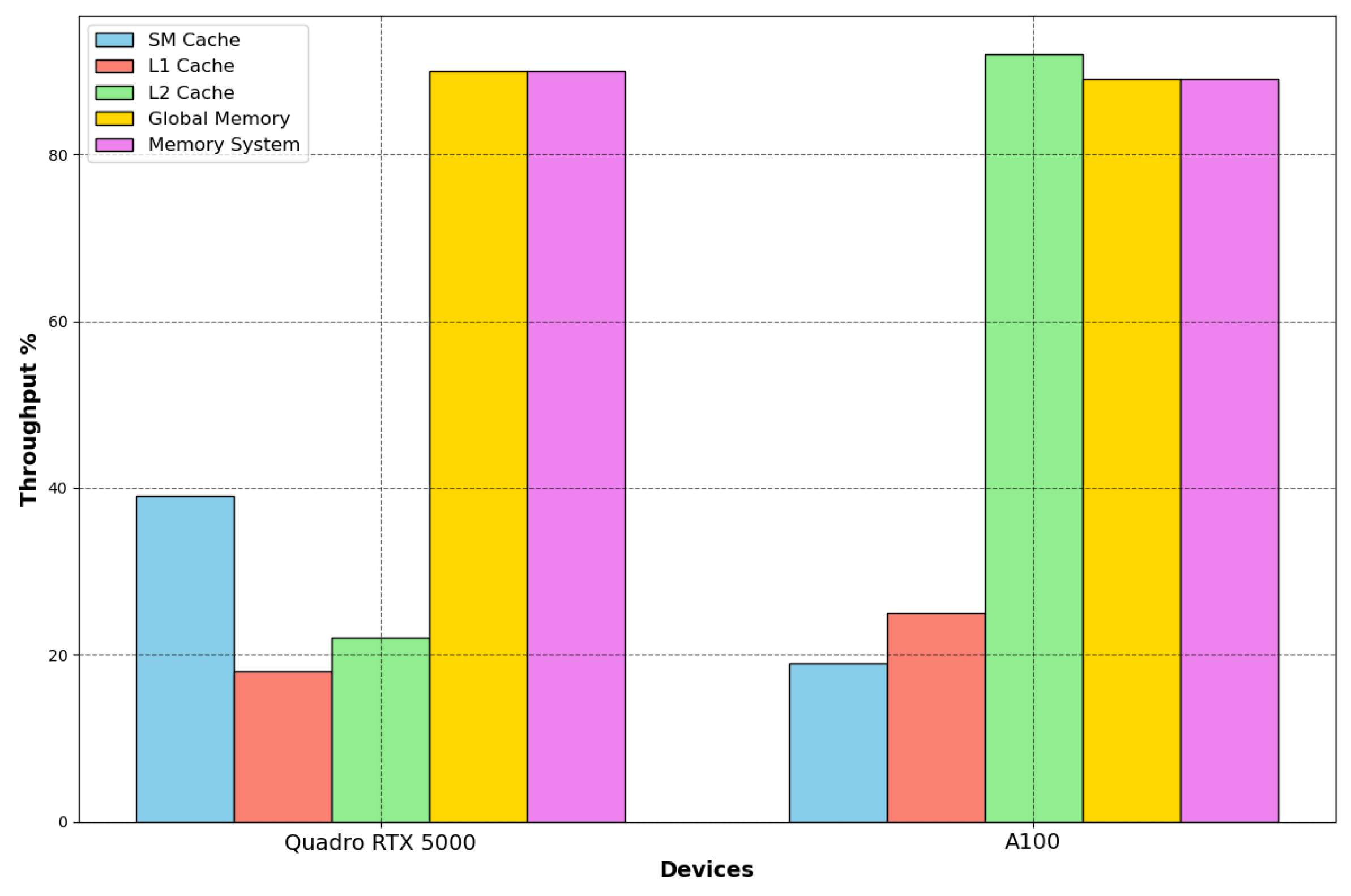
NVIDIA Nsight compute offers features to evaluate the achieved percentage of utilization of each hardware component with respect to the achieved maximum. In
Figure 13, we compare these throughputs on the two devices.
The A100 GPU has 40 MB of L2 cache, which is 10 times larger than Quadro’s L2 cache. The increase in the L2 cache size improves the performance of the workloads since larger portions of datasets can be cached and repeatedly accessed at a much higher speed than reading from and writing to HBM memory, especially the workloads that require a considerable memory bandwidth and memory traffic, which is the case for this kernel. Moreover, the main memory bandwidth is intensively used by the kernel on both architectures, while the SM throughput is low, which helps us in determining the kernel’s bottleneck on GPUs. The compute units are not optimally used; architecture optimization would also greatly improve the GPUs’ compute throughput regarding the Tensor and CUDA cores.
5.2. Optimization Results
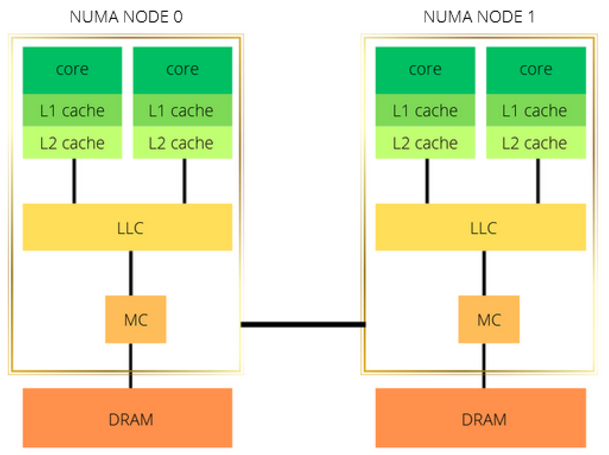
In order to understand the impact of thread binding and affinity, we present the different elapsed times of GRICS with different configurations using only OpenMP. The elapsed time of the code is insensitive to the variable OMP_PLACES. Hence, we choose to bind the threads to hardware threads. However, the elapsed time is remarkably sensitive to the binding strategy.
- -
OS OMP: Only OpenMP parallelization over the receiver coils is considered, with basic optimization flags and without thread binding. The GNU C++ compiler is considered.
- -
Close OMP: The thread affinity is enabled with the close option.
- -
Spread OMP: The thread affinity is enabled with the
spread option. In the three cases, the compilation flags discussed in
Section 4.4.1 are enabled.
Each OpenMP configuration for each dataset is executed five times; the reported time is the mean of the five experiments. Since we are the only user at the workstation while conducting the testing, the differences in the execution times between multiple runs (for a given binding strategy) are not significant: the standard deviations range from 0.30 s to 1.001 s. The thread binding and compilation flags do not impact the numerical accuracy and stability of the program since the number of conjugate gradient iterations remain the same with spread/close bindings: 4, 5, 4, and 11 iterations, respectively, for , and .
Moreover, we compute the Normalized Root Mean Square Error to prove that there is no image quality degradation with the proposed optimizations: , and stand, respectively, for the reconstructed images with the spread, close, and no binding options; we calculate max(NRMSE(), NRMSE(), and NRMSE()). These values are, respectively, equal to 4.67 , 5.95 , 4.89, and 2.40 for , and .
Thread binding and affinity decisions (spread or close) are architecture-dependent for the same program. Using
Table 6, we can see that, on the AMD EPYC processor, the
spread option enables a gain of 9–17% on the AMD EPYC CPU, while the
close option degrades the performance compared to the OS allocation. On the Intel CPU, the code is much slower, and the
close option yields better results compared to the
spread binding. However, the OS thread allocation is more suitable to the GRICS on this architecture.
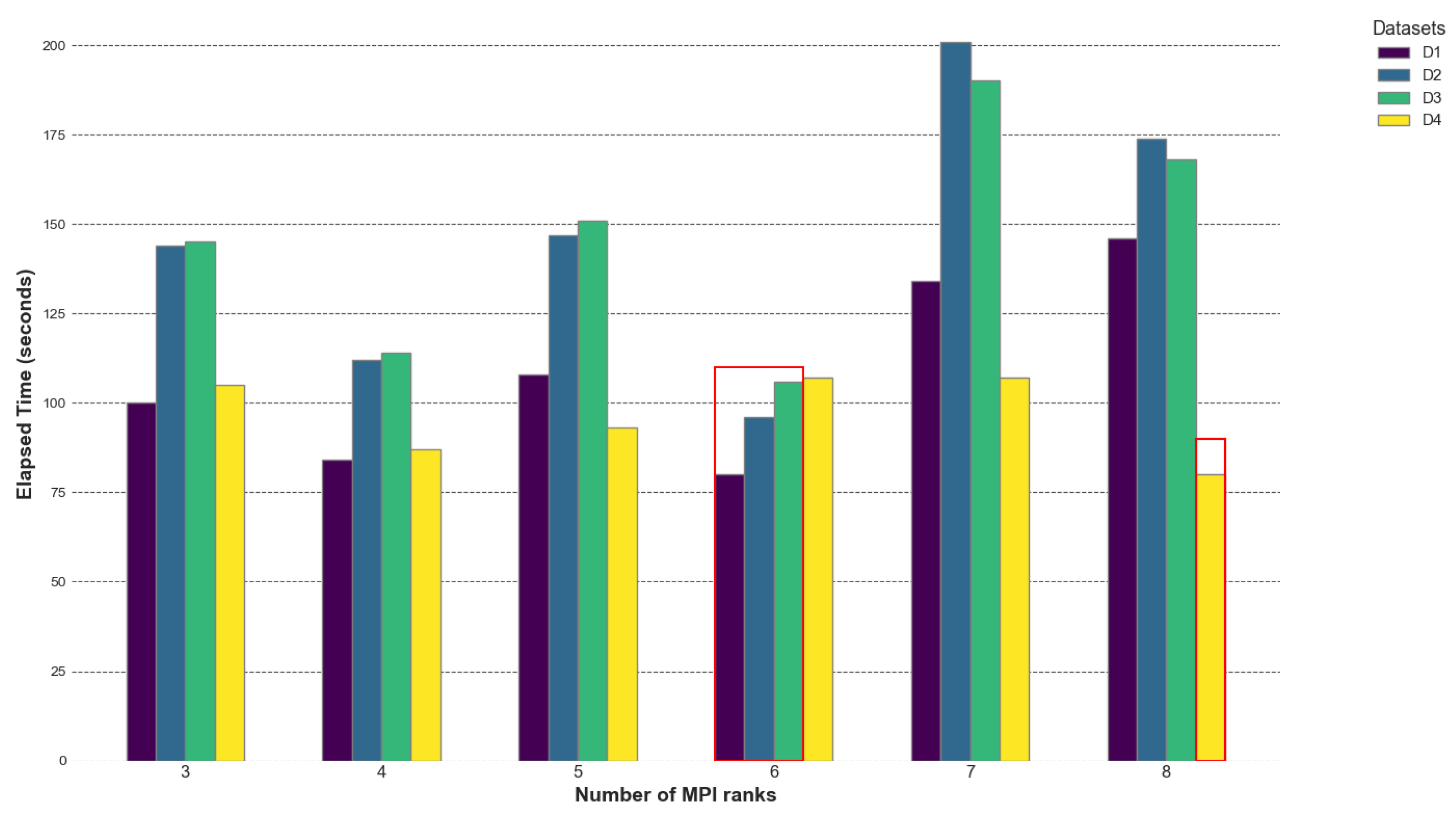
The roofline analysis and the performance of the GRICS’s OpenMP version prove that the EPYC CPU is more suitable for the code, notably in terms of its demanding data traffic. The high value of EPYC’s DRAM bandwidth accelerates the rate at which the data are transferred to the compute units and enables rapid execution. For these reasons, we decided to investigate the performance of the hybrid version only on the AMD EPYC CPU; the different execution times are presented in
Figure 14.
The GRICS’s hybrid implementation improves the overall performance in terms of elapsed time. The best performances are achieved when the number of MPI processes n divides the number of motions states ; for datasets , and , is equal to 12 and the minimal times are reported for . The best performance is achieved with ranks. For dataset with , the minimal elapsed time corresponds to the and processes. When the number of processes n divides the number of motion states evenly, it leads to better load balancing. Each process receives an equal share of the workload, minimizing idle times. The empirical data show that the elapsed time initially decreases with increasing processes (up to a certain point) and then starts increasing. More processes may increase the number of communications required, leading to higher network traffic and contention. For the OpenMP parallelization of the loop over the coils, choosing a number of threads m such that m divides does not greatly improve the overall performance; the set of threads m when provides approximately the same result. A small improvement is noticed when . The best MPI OpenMP settings are and for all the datasets.
Finally, we present in
Table 7 a performance-based comparison between the CPUs and GPUs for the reconstruction kernel. The reported times correspond to the best parallelization strategy for each device; we use dataset
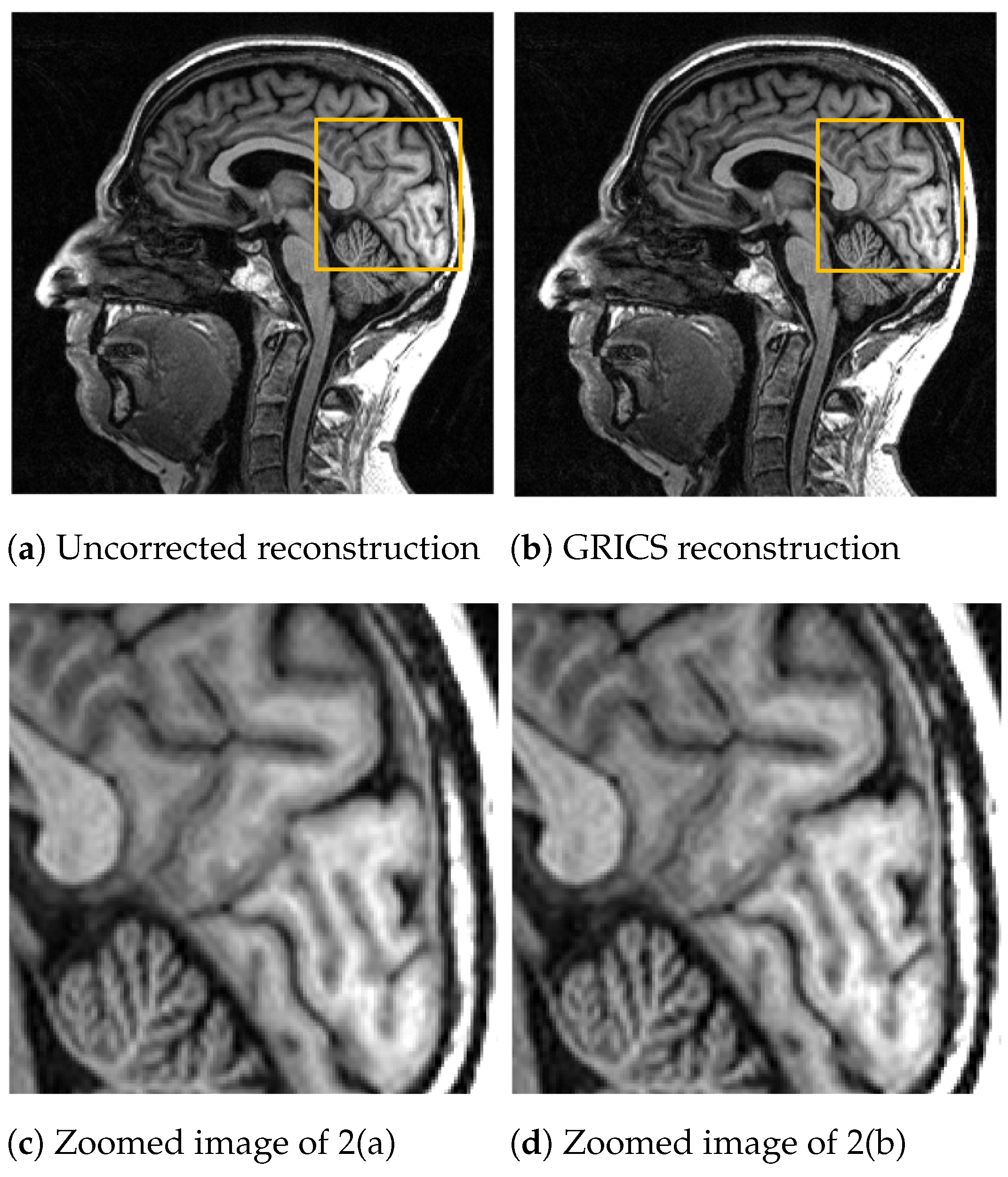
. There is no significant difference between the MRI images from the CPUs and GPUs. Setting
and
as the reconstructed images using the CPU and GPU, respectively, the Normalized Root Mean Square Error of the two images, NRMSE
, is equal to
, which is less than the tolerance of the reconstruction solver (
).
From an architectural perspective, the kernel and GRICS operate well on an AMD EPYC CPU. The roofline analysis on the A100 GPU and the kernel’s elapsed time on this architecture provide us insights about the possible benefits of a full GPU implementation of the GRICS. Even if the actual one is not “GPU architecture aware”, its result is promising. On Quadro RTX5000, the code is slower; Nsight compute reports that L2–DDR data transfer is one of the bottlenecks on this GPU. However, the main hardware limitation on GPUs is the SM’s poor utilization. Both devices offer sophisticated compute capabilities with Tensor cores and CUDA cores, but the actual implementation is not adapted to using the GPU architecture properly, which is why the overall performance values, and , are low compared to . On the Intel Xeon Gold CPU, the code is mainly limited by the low value of memory bandwidth, absence of data reuse, and absence of vectorization.


