A Long-Range Lidar Optical Collimation System Based on a Shaped Laser Source


Abstract
1. Introduction
2. Lidar Detection Principle and System Design
2.1. Lidar Detection Principle
2.2. Lidar System Design
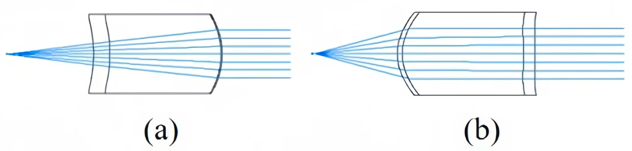
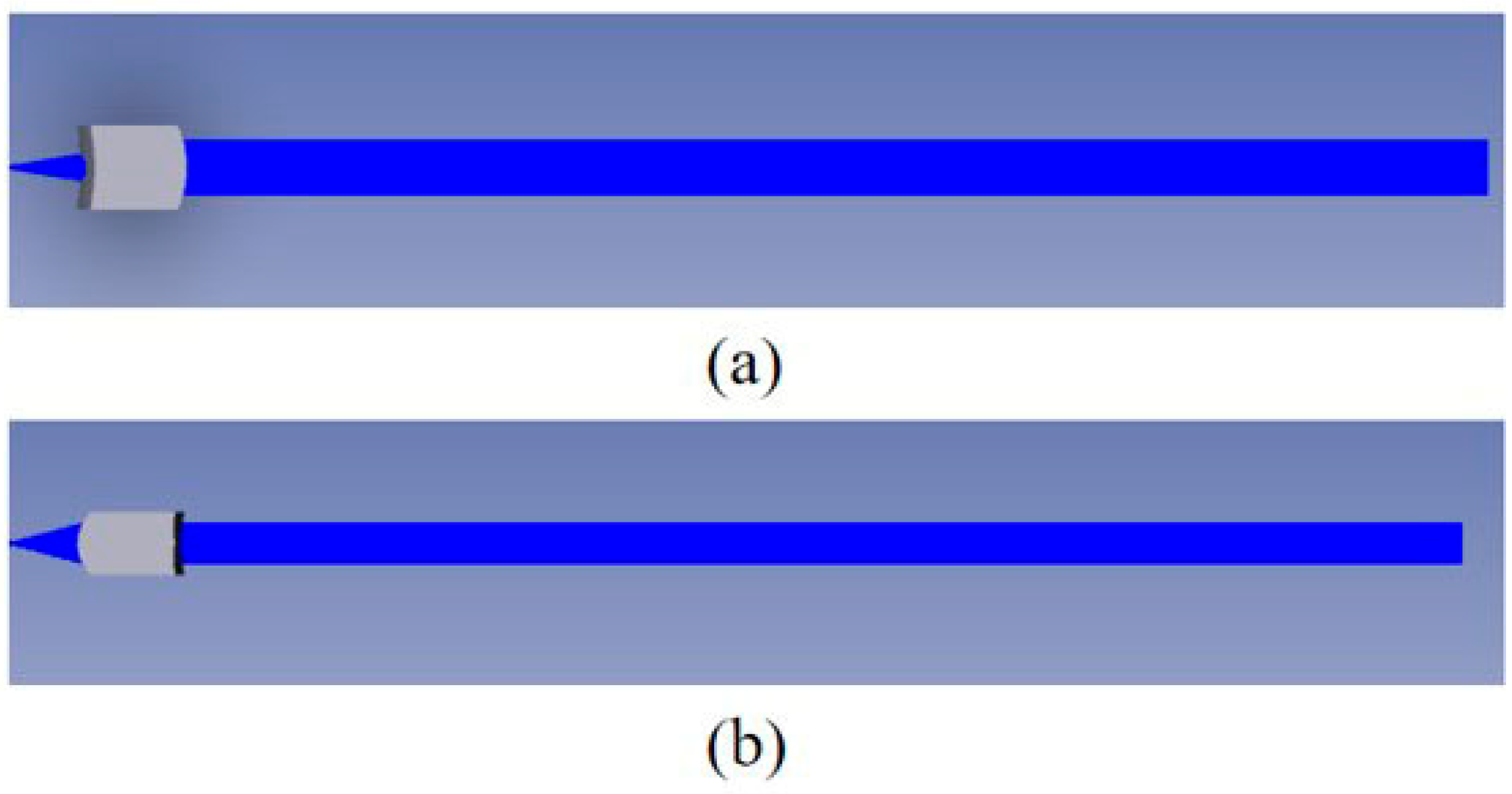
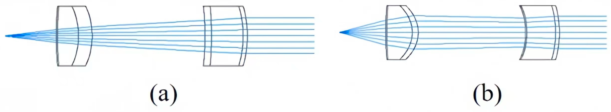
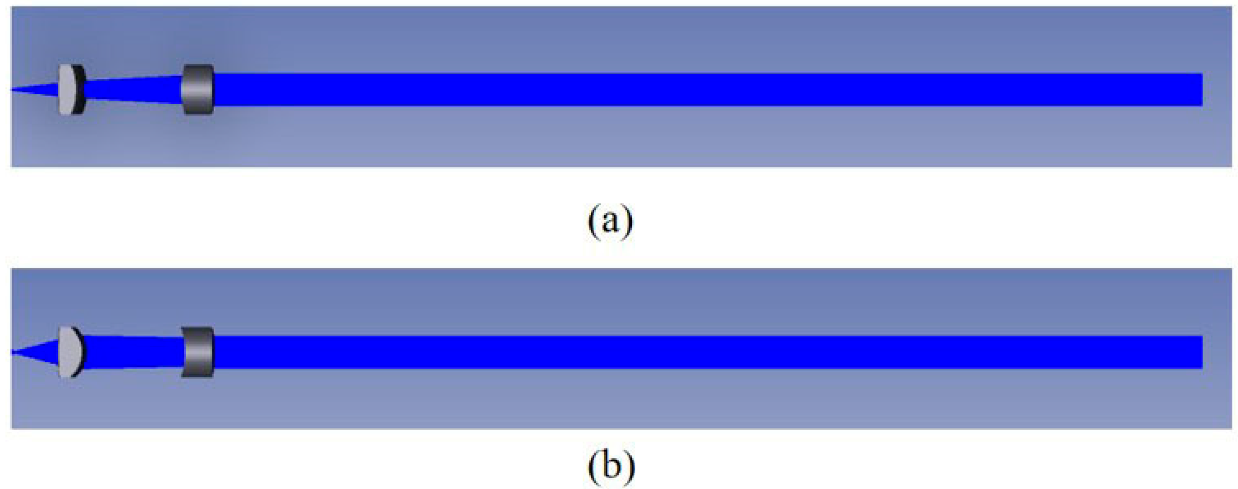
3. Optical Collimation System Design
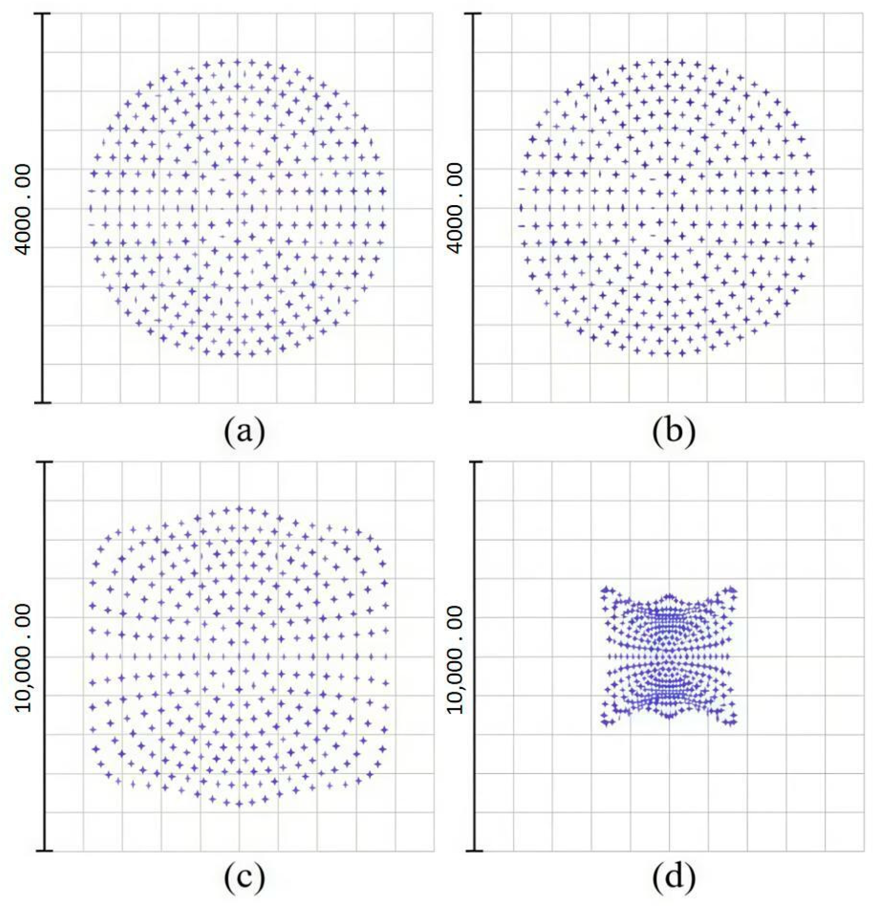
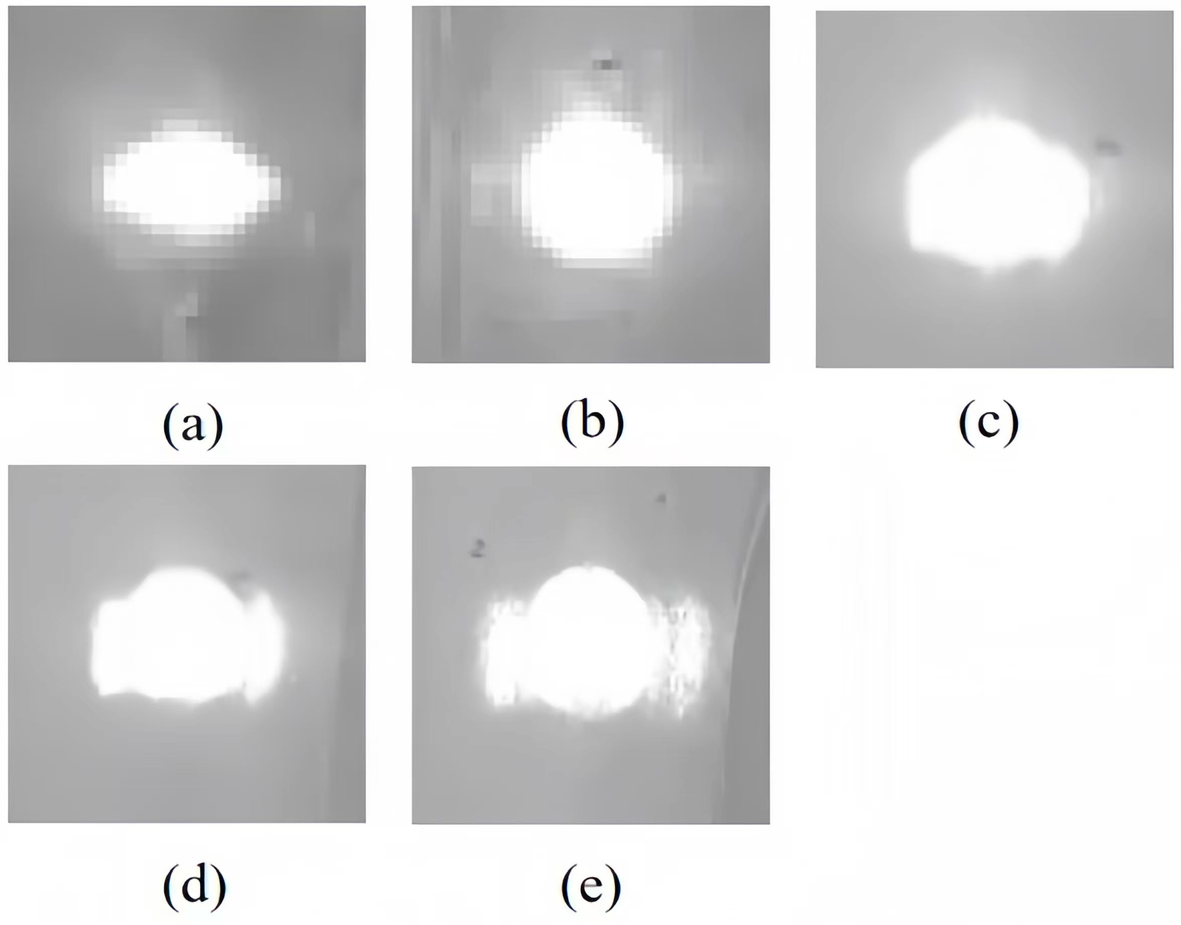
4. Experiments and Data Analysis
5. Conclusions
Author Contributions
Funding
Institutional Review Board Statement
Informed Consent Statement
Data Availability Statement
Acknowledgments
Conflicts of Interest
References
- Molebny, V.; McManamon, P.; Steinvall, O.; Kobayashi, T.; Chen, W. Laser radar: Historical prospective-from the East to the West. Opt. Eng. 2017, 56, 031220. [Google Scholar] [CrossRef]
- Li, K.; Yang, S.; Liao, Y.; Lin, X.; Wang, X.; Zhang, J.; Li, Z. Application of A Frequency Chirped RF Intensity Modulated 532 nm Light Source in Underwater Ranging. IEEE Photonics J. 2020, 12, 1–11. [Google Scholar] [CrossRef]
- Lin, X.; Wu, Z.; Yang, S.; Zhan, Z.; Bi, S.; Zhang, X.; Du, Y. A weak signal detection technique applied in deep space exploration. Infrared Laser Eng. 2017, 46, 913002. [Google Scholar]
- Yong, M.A.; Hang, J.I.; Kun, L.; Hong, L. Application of modulated lidar on optical carrier for ocean exploration. Laser Technol. 2008, 32, 346–349. [Google Scholar]
- Francke, J. A review of selected ground penetrating radar applications to mineral resource evaluations. J. Appl. Geophys. 2012, 81, 29–37. [Google Scholar] [CrossRef]
- Wu, B.; Yu, B.; Huang, C.; Wu, Q.; Wu, J. Automated extraction of ground surface along urban roads from mobile laser scanning point clouds. Remote Sens. Lett. 2016, 7, 170–179. [Google Scholar] [CrossRef]
- González-Aguilera, D.; Crespo-Matellan, E.; Hernández-López, D.; Rodríguez-Gonzálvez, P. Automated Urban Analysis Based on LiDAR-Derived Building Models. IEEE Trans. Geosci. Remote Sens. 2013, 51, 1844–1851. [Google Scholar] [CrossRef]
- Erener, A.; Sarp, G.; Karaca, M.I. An approach to urban building height and floor estimation by using LiDAR data. Arab. J. Geosci. 2020, 13, 1005. [Google Scholar] [CrossRef]
- Horváth, E.; Pozna, C.; Unger, M. Real-Time LIDAR-Based Urban Road and Sidewalk Detection for Autonomous Vehicles. Sensors 2022, 22, 194. [Google Scholar] [CrossRef]
- Ullo, S.L.; Zarro, C.; Wojtowicz, K.; Meoli, G.; Focareta, M. LiDAR-Based System and Optical VHR Data for Building Detection and Mapping. Sensors 2020, 20, 1285. [Google Scholar] [CrossRef]
- Wang, X.; Gao, J.; Zhao, Y. Pollution Monitoring Based on Vehicle-borne Particulate Quantum Lidar. Eur. Phys. J. Conf. 2020, 237, 03023. [Google Scholar] [CrossRef]
- Gao, J.; Wang, X.; Zhao, Y.; Zhao, J. Real-Time Pollution Analysis and Location Based on Vehicle Particle Radar. Eur. Phys. J. Conf. 2020, 237, 03025. [Google Scholar] [CrossRef]
- Suzuki, A.J.; Mizui, K. Bidirectional Vehicle-to-Vehicle Communication and Ranging Systems with Spread Spectrum Techniques Using Laser Radar and Visible Light. IEICE Trans. Fundam. Electron. Commun. Comput. Sci. 2017, 100, 1206–1214. [Google Scholar] [CrossRef]
- Lv, B.; Xu, H.; Wu, J.; Tian, Y.; Zhang, Y.; Zheng, Y.; Yuan, C.; Tian, S. LiDAR-Enhanced Connected Infrastructures Sensing and Broadcasting High-Resolution Traffic Information Serving Smart Cities. IEEE Access 2019, 7, 79895–79907. [Google Scholar] [CrossRef]
- Gong, B.; Zhao, B.; Wang, Y.; Lin, C.; Liu, H. Lane Marking Detection Using Low-Channel Roadside LiDAR. IEEE Sens. J. 2023, 23, 14640–14649. [Google Scholar] [CrossRef]
- Cao, X.; Qiu, G.; Wu, K.; Li, C.; Chen, J. Lidar system based on lens assisted integrated beam steering. Opt. Lett. 2020, 45, 5816. [Google Scholar] [CrossRef]
- Huang, F.S.; Ma, S.; Xue, Z. A rotating two-dimensional laser radar measurement system and the calibration method. Guangdianzi Jiguang/J. Optoelectron. Laser 2018, 29, 987–995. [Google Scholar]
- Chen, Z.; Zhang, J.; Tao, D. Progressive LiDAR Adaptation for Road Detection. IEEE/CAA J. Autom. Sin. 2019, 6, 10. [Google Scholar] [CrossRef]
- Yang, L.; Duan, J. Technology of Vehicle Identification Based on Laser Radar. In Proceedings of the 2011 Third International Conference on Intelligent Human-Machine Systems and Cybernetics, Hangzhou, China, 26–27 August 2011. [Google Scholar]
- Garcia, F.; Cerri, P.; Broggi, A.; Armingol, J.M.; de la Escalera, A. Vehicle Detection Based on Laser Radar. In Computer Aided Systems Theory—EUROCAST 2009: 12th International Conference, Las Palmas de Gran Canaria, Spain, 15–20 February 2009; Springer: Berlin/Heidelberg, Germany, 2009. [Google Scholar]
- Peng, Z.; Liu, B.; Yue, Y. Optical system design of monostatic nonscanning Doppler wind lidar. High Power Laser Part. Beams 2015, 27, 091010. [Google Scholar] [CrossRef]
- Nosov, P.A. Optical system synthesis for lidar transmitting channel. In Proceedings of the International Symposium on Atmospheric and Ocean Optics/Atmospheric Physics, Novosibirsk, Russia, 23–27 June 2014. [Google Scholar]
- Pu, D. Lidar Beam Shaping with Binary Optical Elements. Laser Optoelectron. Prog. 2006, 43, 58. [Google Scholar]
- Xu, F.; Wang, Y.; Yang, X.; Zhang, B.; Li, F. Correction of linear-array lidar intensity data using an optimal beam shaping approach. Opt. Lasers Eng. 2016, 83, 90–98. [Google Scholar] [CrossRef]
- Shealy, D.L.; Chao, S.H. Design and analysis of an elliptical Gaussian laser beam shaping system. Proc. SPIE-Int. Soc. Opt. Eng. 2001, 4443, 24–35. [Google Scholar]
- Zhang, L.; Lu, Q.; Duan, F.; Dai, X.; Qiao, D. Optical System Design and Athermalization of Telephoto Lens. Acta Opt. Sin. 2024, 44, 0822004. [Google Scholar]
- Zhu, Y.; Li, S.; Zhuo, S.; Yang, L. Designing Optical Systems for Close-Distance Vehicle Lenses in Target Recognition. Laser Optoelectron. Prog. 2022, 59, 1722001. [Google Scholar]
- Xu, Z.; Wang, M.; Ju, X. Optimal design of optical system for vehicle navigation LiDAR. Transducer Microsyst. Technol. 2023, 42, 87–90. [Google Scholar]


| Lens Surface | 1 | 2 |
|---|---|---|
| Surface thickness (mm) | 8 | 100 |
| Lens material | PMMA | |
| Net caliber | 2.5 | 2.5 |
| Extended polynomial | : −0.051 : 0.173 | : −0.106 : −0.020 |
| Lens Surface | 1 | 2 | 3 | 4 |
|---|---|---|---|---|
| Curvature radius (mm) | 30.417 | −9.089 | ||
| Surface thickness (mm) | 3 | 10 | 3 | 100 |
| Lens material | PMMA | PMMA | ||
| Net caliber | 2.5 | 2.5 | 2.5 | 2.5 |
| Extended polynomial | : −0.073 : −0.164 | : −0.017 : −0.069 |
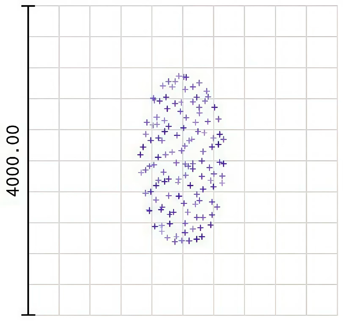
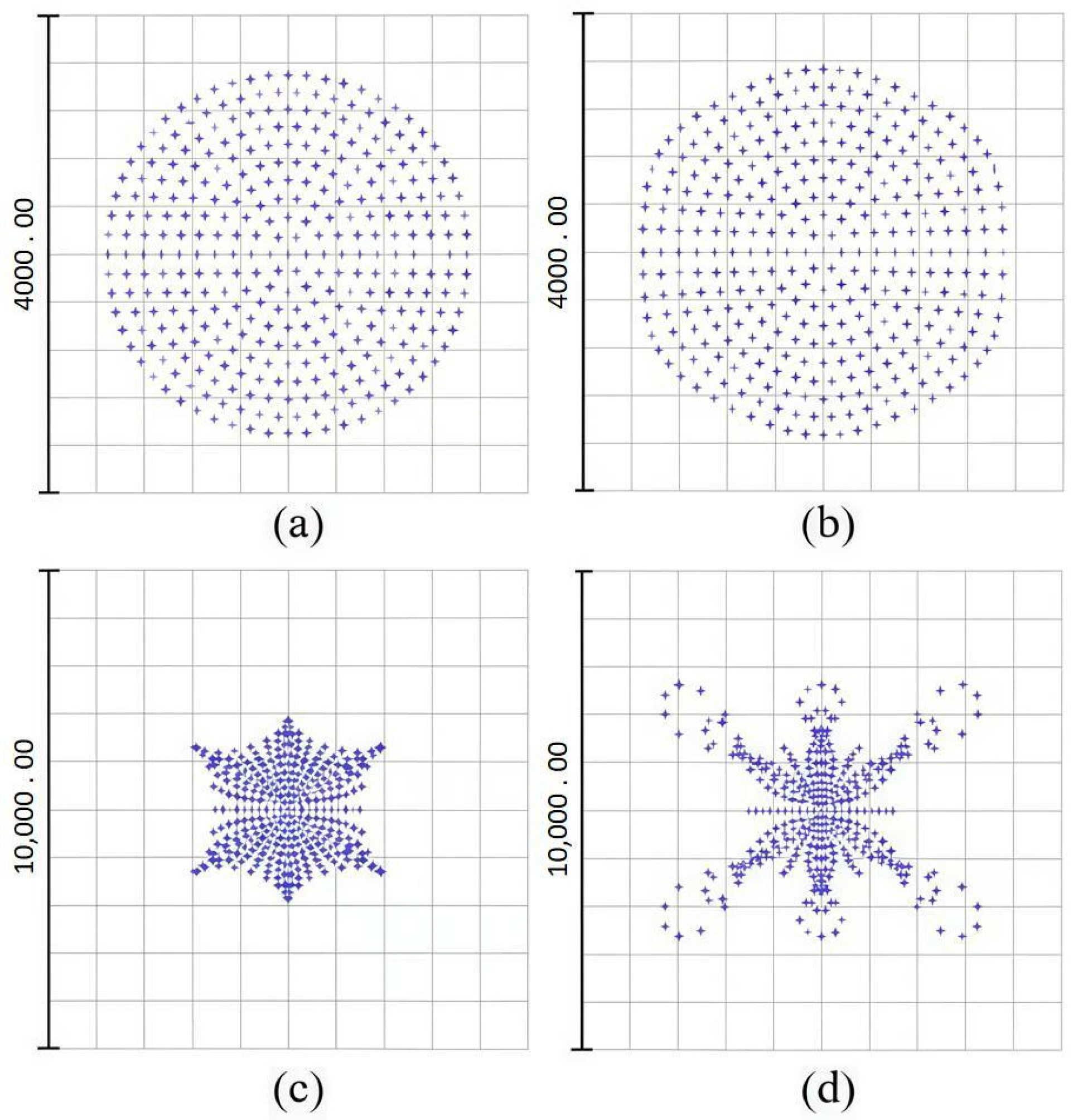
| Ground Glass to Lidar Distance (m) | Spot Shape and Size (Long Side × Short Side mm) | Ground Glass to Lidar Distance (m) | Spot Shape and Size (Long Side × Short Side mm) |
|---|---|---|---|
| 0.5 | 9 × 6 | 3 | 13 × 12 |
| 5 | 19 × 16 | 7 | 22 × 21 |
| 10 | 30 × 29 |
Disclaimer/Publisher’s Note: The statements, opinions and data contained in all publications are solely those of the individual author(s) and contributor(s) and not of MDPI and/or the editor(s). MDPI and/or the editor(s) disclaim responsibility for any injury to people or property resulting from any ideas, methods, instructions or products referred to in the content. |
© 2024 by the authors. Licensee MDPI, Basel, Switzerland. This article is an open access article distributed under the terms and conditions of the Creative Commons Attribution (CC BY) license (https://creativecommons.org/licenses/by/4.0/).
Share and Cite
Feng, S.; Mu, Y.; Liu, L.; Liu, R.; Cai, E.; Wang, S. A Long-Range Lidar Optical Collimation System Based on a Shaped Laser Source. Appl. Sci. 2024, 14, 9662. https://doi.org/10.3390/app14219662
Feng S, Mu Y, Liu L, Liu R, Cai E, Wang S. A Long-Range Lidar Optical Collimation System Based on a Shaped Laser Source. Applied Sciences. 2024; 14(21):9662. https://doi.org/10.3390/app14219662
Chicago/Turabian StyleFeng, Shanshan, Yuanhui Mu, Luyin Liu, Ruzhang Liu, Enlin Cai, and Shuying Wang. 2024. "A Long-Range Lidar Optical Collimation System Based on a Shaped Laser Source" Applied Sciences 14, no. 21: 9662. https://doi.org/10.3390/app14219662
APA StyleFeng, S., Mu, Y., Liu, L., Liu, R., Cai, E., & Wang, S. (2024). A Long-Range Lidar Optical Collimation System Based on a Shaped Laser Source. Applied Sciences, 14(21), 9662. https://doi.org/10.3390/app14219662