Abstract
Motion-compensated image reconstruction enables new clinical applications of Magnetic Resonance Imaging (MRI), but it relies on computationally intensive algorithms. This study focuses on the Generalized Reconstruction by Inversion of Coupled Systems (GRICS) program, applied to the reconstruction of 3D images in cases of non-rigid or rigid motion. It uses hybrid parallelization with the MPI (Message Passing Interface) and OpenMP (Open Multi-Processing). For clinical integration, the GRICS needs to efficiently harness the computational resources of compute nodes. We aim to improve the GRICS’s performance without any code modification. This work presents a performance study of GRICS on two CPU architectures: Intel Xeon Gold and AMD EPYC. The roofline model is used to study the software–hardware interaction and quantify the code’s performance. For CPU–GPU comparison purposes, we propose a preliminary MATLAB–GPU implementation of the GRICS’s reconstruction kernel. We establish the roofline model of the kernel on two NVIDIA GPU architectures: Quadro RTX 5000 and A100. After the performance study, we propose some optimization patterns for the code’s execution on CPUs, first considering only the OpenMP implementation using thread binding and affinity and appropriate architecture-compilation flags and then looking for the optimal combination of MPI processes and OpenMP threads in the case of the hybrid MPI–OpenMP implementation. The results show that the GRICS performed well on the AMD EPYC CPUs, with an architectural efficiency of 52%. The kernel’s execution was fast on the NVIDIA A100 GPU, but the roofline model reported low architectural efficiency and utilization.
1. Introduction
As the power of High-Performance Computing (HPC) systems has been drastically increasing over the years, scenarios of non-optimal use of the processor’s micro-architecture are expected to occur frequently. Programmers must investigate problems from the software and hardware levels. The software performance is mainly controlled by the complex interaction between the compiled code and the micro-architecture of the computing platform [1]. For many scientific intensive-computing applications, the memory bandwidth is the main bottleneck and performance hotspot [2]. HPC systems address this bottleneck by providing local DRAM for each processor node with coherent communication between the nodes and reducing latency through prefetchers. Additionally, they offer remote DRAM in multi-socket systems. However, this memory architecture contributes to a non-uniform memory access (NUMA) phenomenon, which can substantially increase the latency if a thread accesses data that are located on its remote DRAM. NUMA conflicts should be avoided by adjusting the thread and data placement [3]. This complex memory structure and the multiple forms of parallel processing make it hard to completely determine the reasons for a program’s performance. To overcome this complexity, the roofline model was suggested [4]; it is a visual presentation of both the performance bottlenecks of an application and a workstation’s characteristics in terms of memory bandwidth and compute throughput.
The recent advances in Magnetic Resonance Imaging (MRI) algorithms and programs have led to numerous implementation challenges in order to reduce the reconstruction time [5]. To overcome the huge volume of acquisition data, and the computational complexity of such algorithms, CPU and GPU nodes with specific characteristics are required. Many researchers have previously developed efficient solutions with the aim of tackling several MRI reconstruction problems, including non-Cartesian parallel imaging [6,7], compressed sensing [8], and non-linear reconstruction [5]. Moreover, GPU-based systems generally provide larger raw computational power for the same cost and consumption as CPU-only systems, but fully exploiting this potential can be challenging. This is the case for motion-compensated reconstruction, which has higher computational complexity [9,10,11], regardless of whether the correction deals with non-rigid motion, as with GRICS (Generalized Reconstruction by Inversion of Coupled Systems) [12,13], or rigid motion, as with DISORDER (Distributed and Incoherent Sample Orders for Reconstruction Deblurring using Encoding Redundancy) [14,15]. Some researchers have worked on accelerating motion-compensated reconstruction; however, only the motion estimation part of the algorithm was modified with a deep learning approach, whereas a classic optimization was still used for the image reconstruction part [16,17,18]. This limitation may be due to the challenge of generalizing deep-learning-based approaches over different types of MRI datasets. Huttinga et al. proposed a model-based framework to estimate motion, leveraging a reference image to inform the motion model. The authors suggested an efficient GPU implementation to estimate non-rigid 3D motion in real time (with low latency) from minimal k-space data [19]. However, this method was designed for interventional MRI applications rather than high-resolution images; its principal aim was to estimate 3D motion with a small number of parameters, which is a less complicated optimization problem compared to a complete motion-compensated reconstruction task.
The remainder of the article will be focused on the GRICS code but would be applicable to other motion-compensated reconstruction programs. Roughly speaking, the problem size (reconstruction time and memory size) scales linearly with the number of motion states in the model (typically, the authors use eight motion states or more) and with the number of coil receiver channels (20–30 channels are commonly used). Efficient parallelization inevitably leads to large memory overheads; therefore, the total amount of available memory is still a limitation with GPU-based systems for 3D motion-compensated reconstruction in MRI. CPU-only architectures, using multiple cores, also have several advantages in addition to their superior memory space. They are easier to program and are highly portable across architectures and manufacturers (using C or C++ language), unlike GPU-based architectures (e.g., a wide community of developers use CUDA, a vendor-specific language, rather than the OpenCL standard). P. Chen et al. [20] revisited the role of CPUs in image reconstruction problems, a choice that was motivated by power, low-cost, and space requirement considerations. The authors demonstrated that an ARM CPU outperformed high-end GPUs in the Computed Tomography domain. Roujol et al. conducted a comparative analysis of a real-time reconstruction of an adaptive TSENSE across CPU and GPU hardware [21], highlighting the significant acceleration achievable with GPUs. However, they did not explore the potential benefits of integrating and combining multiple parallelization paradigms on CPUs. Inam et al. introduced a GPU-accelerated Cartesian GRAPPA reconstruction using CUDA [22], which was 17 times faster than their CPU multicore implementation. It is worth noting that the CPU code utilized only eight threads, whereas the CUDA implementation used a considerably larger number of threads. This comparison may not be entirely fair since it compromises the possible benefits of massively parallelizing the application over a large set of CPU cores. Wang et al. conducted a survey of GPU-based acceleration techniques in MRI reconstruction [23], emphasizing one of the distinguishing features of GPUs: their superior memory bandwidth. Nevertheless, it is essential to recognize that recent CPUs are also designed with high memory bandwidth and a considerable number of cores, each capable of executing one or more threads. Indeed, CPU-only solutions may involve different parallelization strategies, including nested loop parallelization, e.g., using the MPI and OpenMP, for which many optimizations may be performed without changing the algorithm code. This can be achieved through the investigation of the interaction between the code and micro-architecture, as well as the optimization of specific parameters during both the compilation and execution stages. To our knowledge, these HPC concepts have not yet been applied to the field of MRI reconstruction.
In this work, we investigate the performance of a GRICS in terms of Floating Point Operations (FLOPs) per second and the elapsed time. The performance study is conducted on two different CPU platforms, Intel Xeon Gold and AMD EPYC. We quantify the code’s performance on each architecture and draw conclusions regarding its potential bottlenecks. Furthermore, we assess the optimization patterns of the GRICS’s execution on CPUs, focusing on two patterns: thread binding and affinity in the OpenMP implementation and the optimal combination of MPI processes and OpenMP threads in the hybrid implementation. To draw comparisons about the code’s behavior across architectures, we suggested a MATLAB-GPU implementation of the GRICS’s reconstruction kernel. MATLAB’s version was R2023a. Despite evaluating the performance of the entire program on the CPUs, this comparison remains valid. This is because the reconstruction kernel typically accounts for 70–80% of the GRICS’s elapsed time depending on the considered dataset. Hence, the GRICS’s behavior on CPUs/GPUs would be close to the reconstruction kernel’s behavior, and the roofline analysis regarding the model would be similar. Two NVIDIA GPU devices are considered: Quadro RTX 5000 and A100.
2. Theory
2.1. Joint Reconstruction of an Image and a Motion Model
A review of motion-compensated reconstruction methods can be found in [11]. In this work, motion-compensated reconstruction was accomplished using GRICS [12]. The algorithm solves for both a motion-corrected image and the parameters of a motion model . The GRICS problem is mathematically formulated as follows:
m stands for the acquired MRI k-space data; m is a vector of size . is the motion-corrected image, a vector of elements. u is the displacement field at each k-space sample time; it is a vector of elements, where is the number of dimensions in the image (. In the case of a rigid motion model (e.g., for cerebral imaging), is an affine transformation matrix using homogeneous coordinates. In the case of a non-rigid motion model (e.g., for chest or abdominal imaging), a separable motion model is used, with a spatial component , and the temporal component is a motion signal, acquired from a motion sensor (here, a pneumatic respiratory belt). A regularization term is added in the non-rigid case as . E is an encoding operator; it is expressed using the following operators:
The acquisition is subdivided into motion states (shots) and receiver coils. For a given , each motion state is described by a dense displacement vector field and a sparse spatial transformation matrix . The size of is . The matrices describe the sampling pattern of the k-space data during the motion state. In the Cartesian sampling case, represents sparse matrices, having 0 and 1 as elements. The matrix has columns, and its number of rows is the number of k-space samples acquired at each shot . F stands for the Fourier transform operator. represent the diagonal coil sensitivity operator of the receiver coils. For each , the size of the matrices and operator F is . In GRICS, the Fast Fourier Transform of a vector is computed using the FFTW implementation [24].
The two least squares problems in Algorithm 1 are solved using the conjugate gradient solver. The Gauss–Newton scheme is introduced to linearize the cost function, line 8 around the current estimate of ; each iteration suggests a refinement of . The tolerances are for the reconstruction solver and for the motion problem. In the last resolution level, only the reconstruction step is performed.
| Algorithm 1 Joint reconstruction with GRICS. |
|
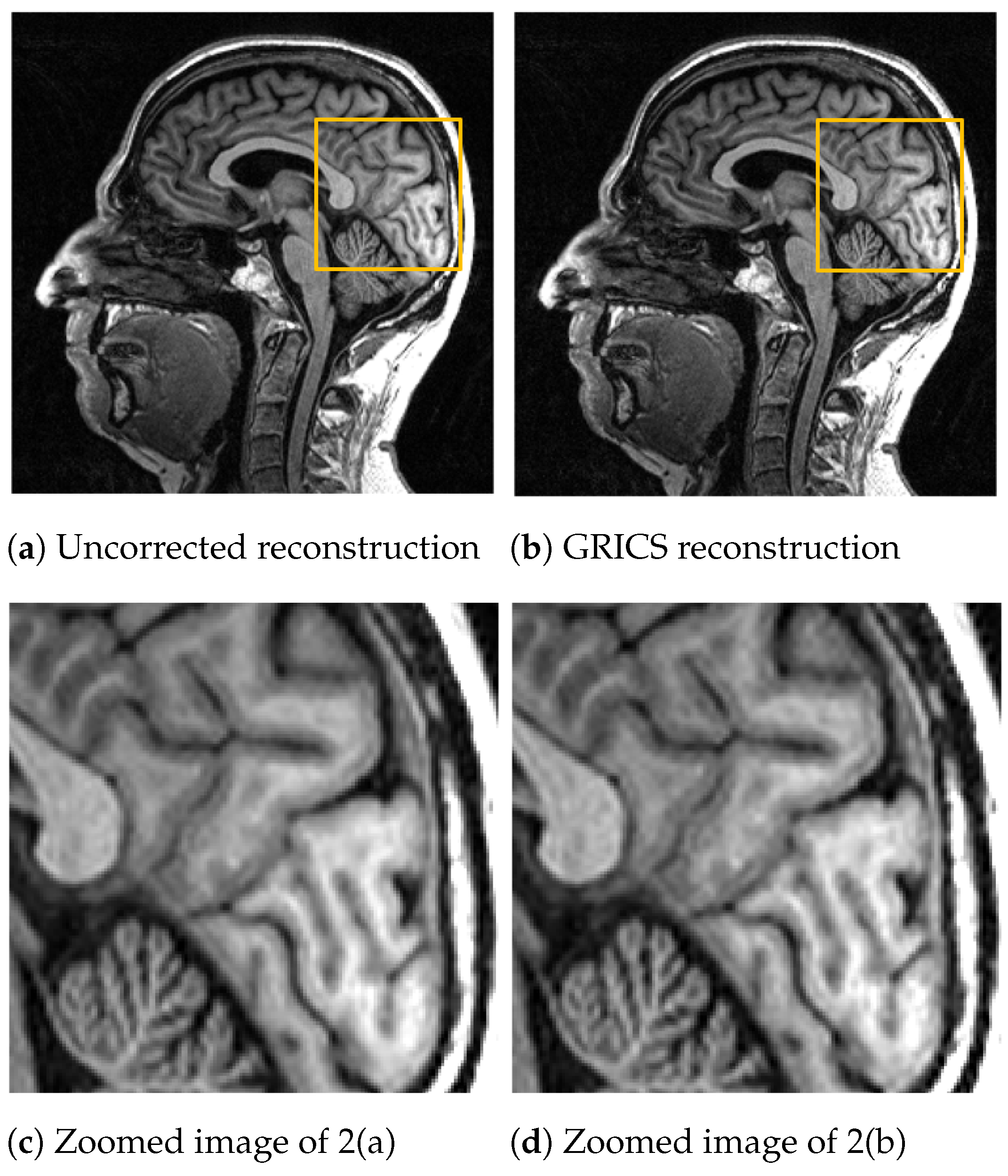
For the generalized reconstruction problem, we set . For the model optimization, we choose . The coil sensitivity maps are computed from the central lines of k-space data with 24 calibration lines and smoothed with second-order splines with a smoothing factor for both magnitude and phase. Examples of GRICS reconstruction are presented in Figure 1 and Figure 2. Figure 1 illustrates a non-rigid motion-compensated breast MRI reconstruction, where we can see an improvement in the reconstruction quality compared to the uncorrected reconstruction. Figure 2 demonstrates a rigid motion-compensated brain MRI reconstruction. The patient was instructed not to move; hence, there was no significant difference between the uncorrected and motion-corrected images. The overall maximum amplitude of motion was: 1.55 degrees for rotation and 0.7 mm for translation, indicating that the motion was minimal.
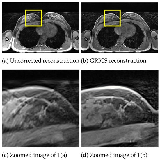
Figure 1.
Comparison between a reconstruction without motion correction and the GRICS reconstruction. GRICS minimizes the motion artifact, dataset .

Figure 2.
Comparison between a reconstruction without motion correction and GRICS reconstruction. Sixteen motion states were considered, dataset . This MRI acquisition was conducted without obvious motion. For quantitative comparison, we determined the sharpness index [25] of the images. The index was equal to for the uncorrected reconstruction and for the corrected reconstruction.
The most computationally intensive part of Algorithm 1 lies in the conjugate gradient linear solvers. In particular, the application of the operator , where is the Hermitian transpose of the operator E-, comprises an outer loop on motion states and an inner loop on coil receivers. Algorithm 2 briefly presents the structure of this part of the kernel for the reconstruction problem. The operator reads
For the motion model problem, we have a similar intense computational part with the application of the operator , where J is the Jacobian matrix. Demo codes in MATLAB can be downloaded here: http://freddy.odille.free.fr/2023/02/motion-corrected-mri-reconstruction/ (accessed on 6 May 2024).
| Algorithm 2 Bottleneck of the reconstruction step (function ). |
|
2.2. The Roofline Model
Initially proposed by S.Williams et al. in 2008, the roofline model [4] is a throughput-oriented performance model. It aims to visualize the performance P of a code on a specific micro-architecture. The model provides insights on how to improve the overall performance of a given program, on its main bottlenecks, and can provide the developer a vision of the most adapted architecture to his code.
The roofline model relies on three main concepts:
- -
- The peak performance of the CPU/GPU, which can be defined as the maximum speed at which all the components of a machine can operate [26]. In a considerable number of application codes, this limit is never reached. In this work, is expressed in terms of GFLOP/s.
- -
- The main memory bandwidth , which is the rate at which data can be transferred from memory to CPU/GPU [26]. It is expressed in GB/s. In several scientific programs and modeling applications, DRAM bandwidth is considered the main bottleneck. Memory specifications refer to that a certain memory chip can achieve. However, this theoretical bandwidth requires perfect circumstances and is not attainable in reality [2].
- -
- The operational intensity I of a program; this metric characterizes the code itself, while the machine is characterized by and . I is defined as the ratio between the number of operations performed by a given kernel and the number of bytes of memory transferred from a memory level to the computing unit. In our case, the operations refer to Floating Point additions and multiplications. Hence, the operational intensity is expressed in FLOP/byte.
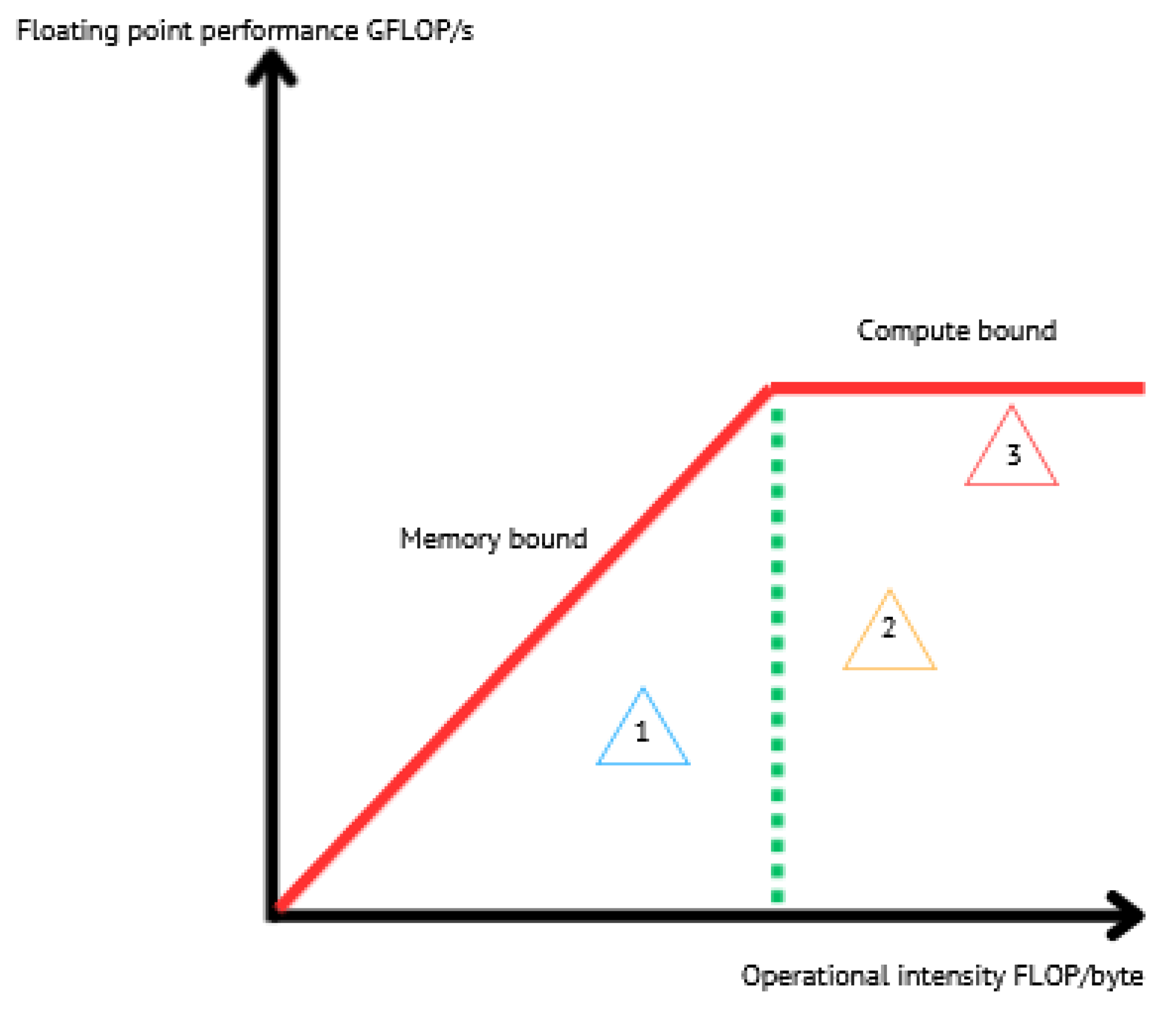
The graph of the roofline model is on a log–log scale, the X-axis is FLOP/byte, and the Y-axis is GFLOP/s. The peak Floating Point performance of the machine is expressed as a horizontal line or ceiling. The peak memory performance is considered as the maximum FLOP performance that the memory can provide for a specific value of the operational intensity I. The peak memory performance is represented by a line at a 45-degree angle. The two ceilings intersect at the point of peak FLOP performance and peak DRAM bandwidth [4]. They also provide what we call the performance limits by setting upper bounds to the attainable performance of a kernel; see Figure 3. Hence, the performance P verifies the following inequality.
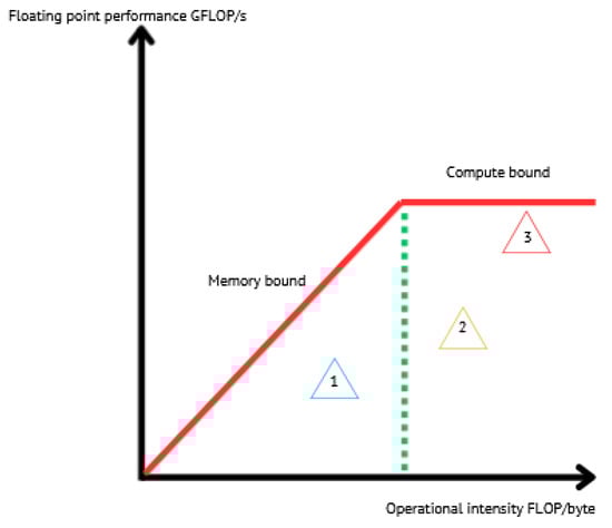
Figure 3.
Sketch of the roofline model. The red lines present performance boundaries. Using the model, kernels are subdivided into two categories: kernels on the left of the green dashed line, which are memory bound, and others on the right of this line are said to be compute bound. Program 1 is memory bound. It is mainly limited by data traffic and memory access. Programs 2 and 3 are compute bound. Program 3 is close to the theoretical upper bound, which means that it uses the micro-architecture in an optimal manner. However, programs 1 and 2 are far from their boundary, not adequately using the micro-architecture.
The architecture efficiency of an application a running on an architecture i is provided by
Conventionally, the roofline model focuses on one level in the memory hierarchy (DRAM or HBM). However, this has been extended to the full memory system, DRAM, HBM, and caches, in order to understand the impact of data locality and reuse. This model provides additional insights into the performance of the memory system [27,28]; see Figure 4.
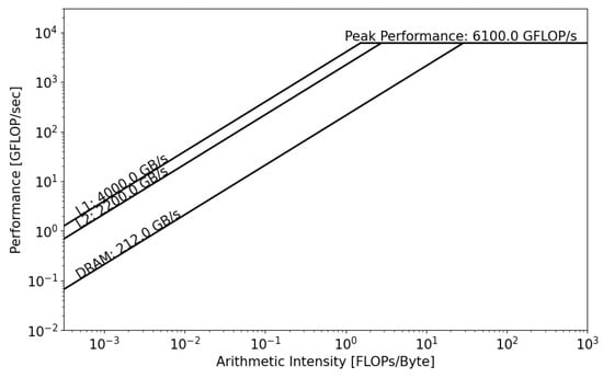
Figure 4.
Example of a hierarchical roofline model with bandwidth of cache levels, main memory, and peak FLOP performance. With this model, the programmer can derive the operational intensity of his program with respect to each memory level. In addition to determining the principal hardware limitations, the programmer can identify some key performance hotspots with this model, such as caching efficiency and data reuse.
3. Parallel Programming and Implementations of GRICS
3.1. Brief Overview of Parallel Programming
Many problems in scientific computing, such as MRI reconstruction, involve the processing of large quantities of data stored on a compute node. In the case where manipulation can be performed in parallel by multiple processors working on different parts of the data—data parallelism—programmers can investigate a parallel implementation of their codes. For this purpose, several parallelization paradigms were suggested.
Open Multi-Processing (OpenMP) is a standard of Shared Memory Parallel Programming; it is a set of compiler directives that a non-OpenMP-capable compiler would just consider as comments and ignore. In a given OpenMP program, the master thread runs immediately after startup; this is the sequential part of the execution. Parallel execution happens inside parallel regions, which are delimited by OpenMP pragmas. Between two parallel regions, no thread except the master thread executes any code. This is called the “fork-join model”. Inside the parallel region, a team of threads executes instruction streams concurrently [26].
The Message Passing Interface (MPI) is the standard implementation of the “Message Passing” model of parallel computing. It is a library of functions that enables data communication between processes or ranks. The parallel computation consists of a number of processes, each working on some local data. Each process has local variables. Data sharing between processes takes place by explicitly sending and receiving data between processes (Message Passing). The MPI is the standard of Distributed-Memory Parallel Programming [26].
Hybrid Programming using the MPI and OpenMP is a well-used parallelization technique that takes advantage of both paradigms. The idea of a hybrid OpenMP–MPI programming model is to allow any MPI process to spawn a set of OpenMP threads in the same way as the master thread does in a pure OpenMP code. In particular, compute-intensive loop constructs are the targets for OpenMP parallelization in a hybrid code. Before launching the MPI processes, one has to specify the maximum number of OpenMP threads per MPI process. At execution time, each MPI rank activates a team of threads whenever it encounters an OpenMP parallel region [26].
For GPUs, parallel codes are often implemented using Compute Unified Device Architecture. CUDA is an extension to the C language that allows GPU code to be written in C language. The code is either targeted at the host processor (the CPU) or targeted at the device processor (the GPU). The host processor spawns multi-thread kernels onto the GPU device. The GPU has its own internal scheduler that will allocate them to whatever GPU hardware is present on the workstation [29].
3.2. Parallel Implementations of GRICS
In this work, three different implementations were considered.
- -
- OpenMP implementation
In the pure OpenMP version of GRICS, the coils are distributed over OpenMP threads by adding pragmas before the loop over coils, line 6 in Algorithm 2. The code is linked to threaded and serial FFTW-3.3.3 package [24], and to the Blitz-0.9 library [30]. There is no nested OpenMP parallelism in GRICS so far. The version of OpenMP is 4.5.2.
- -
- Hybrid MPI OpenMP implementation
In the hybrid MPI and OpenMP version of the GRICS, the coils are distributed over OpenMP threads, and the motion states are distributed using the MPI, line 3 in Algorithm 2. Each MPI process represents an independent computational entity, operating on its allocated subset of motion states . The MPI guarantees inter-process communication and synchronizes computations among distributed processes or ranks. This distributed approach enables efficient workload allocation across the compute node. The OpenMP distribution is created explicitly by adding specific pragmas before the loop over coils. The code is linked to threaded and serial FFTW-3.3.3 package [24], and to the Blitz-0.9 library [30]. The version of the MPI is 4.0.3.
- -
- Preliminary MATLAB–GPU implementation of the reconstruction kernel
In order to draw a comparison with CPU performance, we suggested a preliminary MATLAB–GPU implementation of the reconstruction kernel—the application of the operator , step 6 of Algorithm 1, with iterative calls to Algorithm 2. For this purpose, the MATLAB gpuArray object is used; it enables the storage of arrays on GPU memory, which allows the programmer to run a kernel on GPU with minimal software modifications. In particular, operators of Algorithm 2 were declared as gpuArray. The spatial transformation operator was the only operator that needed to be transferred from CPU to GPU memory at the beginning of each outer loop since their storage for all motion states on the GPU device memory resulted in an out-of-memory error on Quadro RTX 5000, which was not the case on A100). In MATLAB, the gpuArray object supports CUDA, allowing MATLAB to efficiently harness the parallel processing capabilities of GPUs. By using CUDA, MATLAB can offload computationally intensive tasks to the GPU, resulting in speedups for certain types of calculations, particularly those involving large datasets. Additionally, within the framework of the MATLAB Parallel Computing Toolbox, the MAGMA library [31] is used to enhance the performance and accuracy of linear algebra functions designed for gpuArray objects. Furthermore, MATLAB’s execution model incorporates Just-In-Time (JIT) compilation, where code is compiled dynamically during runtime, optimizing performance by converting high-level MATLAB code into machine code. Although this approach is not as efficient as a full native GPU implementation, this JIT compilation process allows MATLAB to apply native GPU libraries to data stored in GPU memory, eliminating unnecessary data transfers between CPU memory and GPU memory. Additionally, we provided as Supplementary Materials a benchmarking of 3D FFT, which is at the core of all iterative MRI reconstruction programs. This provides an estimate of the upper bound of performance that could be achieved if the whole problem could fit in GPU memory.
3.3. Complexity Analysis of Algorithm 2
In this section, we present an analysis of the computational complexity of the reconstruction kernel (Algorithm 2) to identify the reconstruction parameters that contribute most significantly to the computational costs. Let us break the application of the operator into simple multiplication steps:
- Applying : Multiplication of a vector by a sparse matrix of size has a complexity of , where is the size of the interpolation kernel (in our case, we use a linear interpolation kernel ).
- Applying : Same as the application of .
- and its are diagonal matrices, each with a complexity of .
- FFT and its inverse are performed using FFTW implementation, each with a complexity of .
- Assuming that the maximal number of non-zero elements per row in the matrices and is k, where , the complexity of applying and is .
The dominant term for each inner loop of Algorithm 2 is . Hence, each outer loop iteration of Algorithm 2 requires . Finally, the overall complexity is provided by
C can be expressed using the number of k-space samples in frequency and phase-encoding directions, , , and (see Table 1) since .
In our case, the FFT is performed only on the phase-encoding directions; hence, C reads as follows:
Using similar reasoning, we can compute the memory complexity (the amount of memory a program requires to execute relative to the size of the input data) too; reads as follows:

Table 1.
The four datasets in GRICS.
3.4. Communication Complexity Analysis
In order to understand the performance of the MPI, we suggest a process communication analysis. First, each process receives its share of the data for different motion states. The size of data communicated here depends on the number of motion states and the size of the data . The initial distribution of x (line 4, Algorithm 2) to all processes requires sending elements. Hence, the communication complexity of the data distribution is per process. Then, after computing partial results, each process will send its local y (line 9 in Algorithm 2) back to the root process. The communication complexity per process for gathering the vector y is . Summing these contributions, we derive the overall communication complexity .
In terms of the dimensions , , and , reads as follows:
4. Methods
4.1. Data Acquisition
The MRI raw data were acquired on a 3T MR scanner (MAGNETOM Prisma, Siemens Healthineers, Erlangen, Germany). Four healthy volunteers were scanned, resulting in four in vivo datasets. Three datasets with non-rigid motion were acquired with a T1-weighted 3D GRE (fast low angle shot gradient echo) sequence, covering the breast region. The breast MRI acquisition was performed during free breathing, with the subject lying in the supine position. Further details about the imaging protocol can be found in [32]. A dataset with subtle rigid motion was acquired using a T1-weighted 3D MPRAGE (Magnetization-Prepared Rapid Gradient Echo) sequence covering the head. The study was conducted in accordance with the ethical principles outlined in the Declaration of Helsinki (1975, revised 2013) and was approved by the ethics committee (approval number: [CPP EST-III, 08.10.01]) under the protocol “METHODO” (ClinicalTrials.gov Identifier: NCT02887053). All participants provided written informed consent prior to their inclusion in the study.
The main parameters of the dataset of GRICS are the number of samples in frequency encoding direction, , in phase-encoding direction in the image plane, , and in the direction of slices, . The size of the matrix is . The number of coils in the coil array is (“Body 18” and “Spine” coil arrays from the manufacturer; “Head 20” for brain MRI data); the number of shots or motion states is . In this work, the acquisition type is 3D.
The datasets were carefully chosen by selecting different cases with varying coil numbers and dimensions. The study aims to comprehensively evaluate and understand the impact of these variables on the performance. Specifically, the datasets include different combinations of , , , , and , reflecting real-world scenarios with distinct spatial resolutions and complexities.
4.2. The Test Machines
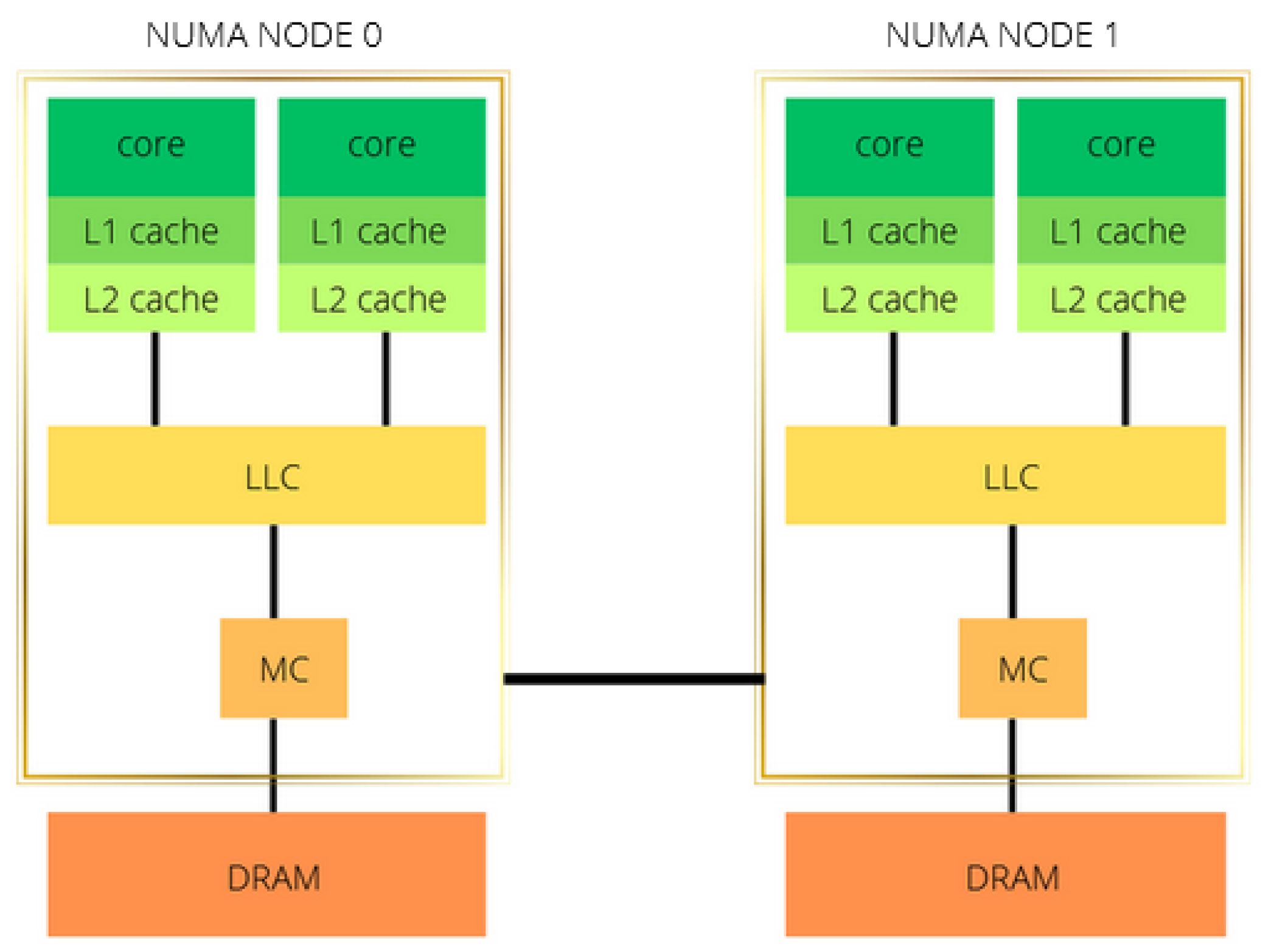
GRICS was executed on two CPU architectures, Intel Xeon Gold 5220 and AMD EPYC 75F3 processors. The CPUs have a sensibly similar architecture layout: two NUMA nodes and two sockets; the cores of each socket have private L1 and L2 level caches and share the L3 level cache; see Figure 5 and Table 2.
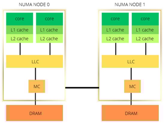
Figure 5.
Modeling of a two-socket, two-NUMA-node architecture. LLC stands for the last-level cache, which is shared between all cores of the same socket/NUMA node. MC is the memory controller, and DRAM is the main memory.
Table 2.
The characteristics of the CPUs.
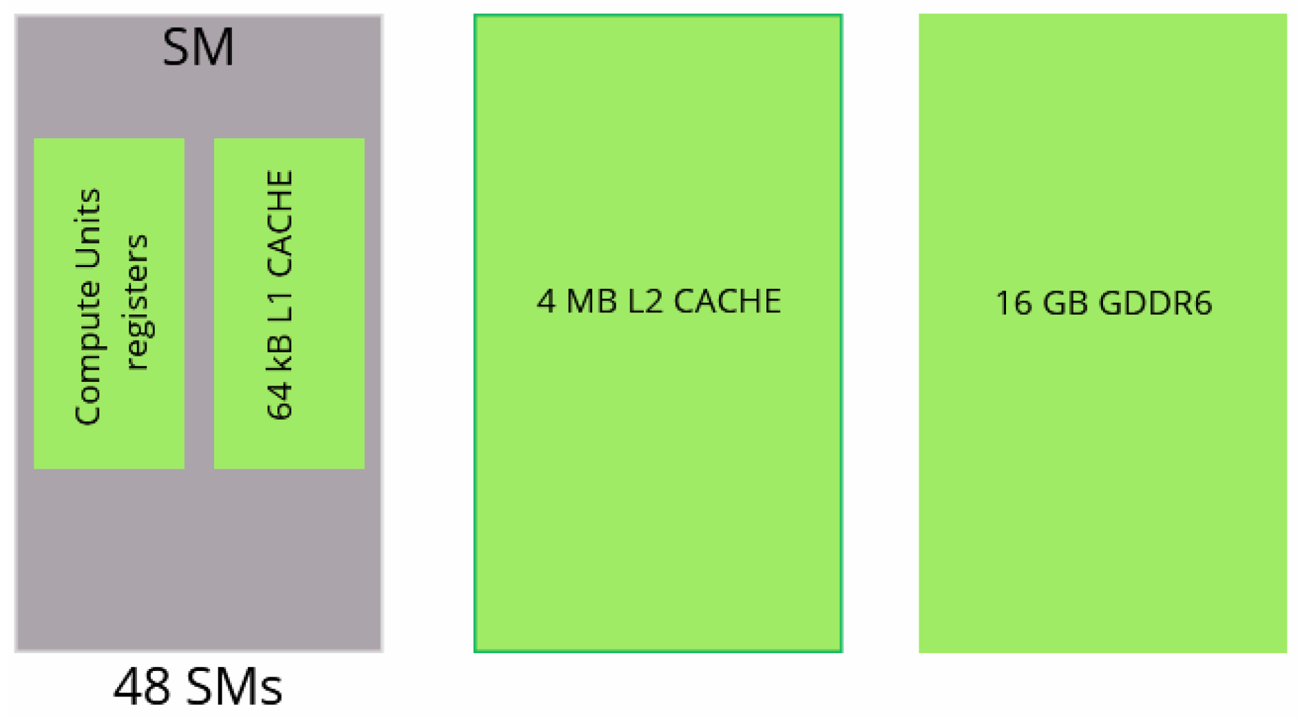
Moreover, two GPU architectures are considered, NVIDIA Quadro RTX 5000 and NVIDIA A100. Sketches and characteristics of the two GPUs are presented in Figure 6 and Figure 7 and Table 3.
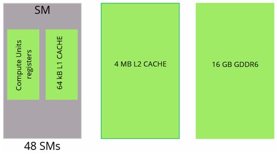
Figure 6.
Modeling of NVIDIA Quadro RTX 5000 GPU.

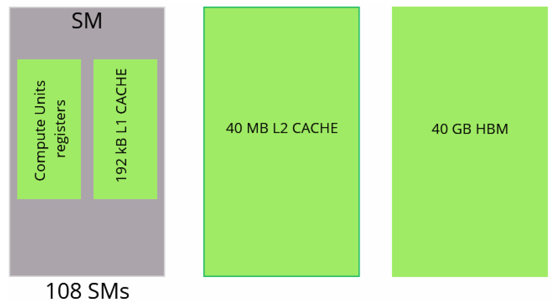
Figure 7.
Modeling of NVIDIA A100 GPU.
Table 3.
The characteristics of the GPUs. SM stands for Streaming Multiprocessor. SMs are akin to CPU cores.
4.3. Analysis Methods
4.3.1. The Empirical Roofline Toolkit ERT
In order to generate the roofline model, theoretical values of peak performance and DRAM/HBM bandwidth could be used, but they will not provide realistic modeling of the architecture–code interaction. In this work, we used the Empirical Roofline Toolkit ERT-1.1.0 [33]; the tool generates the required characterization of a machine empirically. It does this by running specific kernel codes on the test machine so that the results are attainable in reality by some codes. The ERT generates the bandwidth of the DRAM/HBM and cache levels and estimates the empirical peak performance of the CPU/GPU device. The input of the ERT is a configuration file where the user mentions machine specification data and the final output is the roofline chart in Postscript format and the roofline parameters in JSON format. The ERT is employed to gather the empirical values of memory bandwidth and peak performance. Then, we used the NERSC-Roofline repository [34] to generate the final plot with GRICS information in terms of operational intensities and achieved performance.
4.3.2. Application Characterization
On HPC systems, the programmer must deal with the complexity of the hardware, the different parallelization paradigms, network topology, and software builds. Hence, it is important to quantify the application’s performance, using performance profiling tools, to see whether it is possible or not to obtain a better performance on the same system. These tools generate different performance metrics, identify hotspots for code, and help in the determination of adequate optimization techniques. We present the tools used to profile the code on the considered architectures:
- -
- Intel Vtune and Intel Software Development Emulator
Intel Vtune-19.0.4 [35] and Intel SDE-9.14 [36] are used to profile the code on Intel architecture. In particular, the SDE tool can be employed to collect the number of FLOPs and the L1 data movement. Vtune is used to capture data traffic in DRAM and cache levels [37]; the total bytes are read and written in each memory level. Then, the achieved performance on the architecture i is = SDE FLOPs/T, where T is the application’s elapsed time. The operational intensity of the code regarding a specific memory level is = SDE FLOPs/Vtune_Bytes_, where Vtune_Bytes_ is the number of Vtune memory accesses (read and write) for the memory level .
- -
- AMDProf
AMDProf-4.1 [38] is used to characterize the performance bottlenecks in the source code and to identify ways to optimize it on AMD architecture. The tool integrates a roofline support in order to generate the roofline data and the roofline plot. The achieved performance on the architecture and the operational intensity of the DRAM are reported in the roofline support, while for a memory level we have = Prof FLOPs/Prof_Bytes_, where Prof_Bytes_ is the number of Prof memory accesses (read and write) for the memory level .
- -
- NVIDIA Nsight Compute
Nsight Compute [39] is employed to collect performance data on Nvidia GPUs. It provides a set of metrics to evaluate in order to compute the number of FLOPs and data movement. We summarize the metrics for roofline data collection in Table 4.
Table 4.
NVIDIA Nsight compute metrics. FP stands for Floating Point. In the following, will stand for sm__sass_thread_inst_executed_op_fpprec_pred_on.sum, where prec , stands for sm__inst_executed_pipe_tensor.sum, and for the memory level metric, where {L1, L2,HBM}.
The total number of FLOPs = + + + 512, the achieved performance on GPU architecture i is = FLOPs/T, where T is the kernel runtime, and the operational intensity of memory level is = FLOPs/.
4.3.3. Memory Footprint
Using Table 5, we define , the total memory footprint of the reconstruction kernel.
In terms of the dimensions , , and , reads as follows:
Using Equation (12), none of the 4 datasets of Table 1 can entirely fit in the cache levels of the studied CPUs/GPUs.
Table 5.
Memory footprint of Algorithm 2. stands for the maximum number of non-zero elements per row. The elements of operator T are pre-computed. stands for the number of physiological signals used to derive the spatial transformation matrix during acquisition. refers to the size of the elements. In GRICS, we work with single-precision float, so bytes (32 bits). FFT is conducted using FFTW implementation, so we do not need explicit storage of the FFT operator F.
4.4. Optimization Methods
The following optimizations were investigated only on CPUs.
4.4.1. Compilation Flags
The choice of the compilation flags is a crucial step: it helps to exploit the hardware specificities and capabilities of a system running a given program or application [40]. GRICS is a C/C++ program; it is compiled with GNU C++ 9.4.0 compiler. The flag -Ofast is applied to provide the highest level of compiler optimizations and to enable automatic vectorization. The flag -fopenmp enables generating parallel code using OpenMP. The -march=native flags instruct the compiler to build binaries optimized for our specific AMD EPYC micro-architecture. We used also the flag -mavx2 to generate codes using AVX2 instructions. Finally, we used the flag -mfma to enable the use of the FMA instructions. For the Intel Xeon processor, we enabled architecture optimization with -march=cascadelake flag, and we used -Ofast too.
4.4.2. Thread Binding and Affinity
The operating system is able to move a thread around from its initial position while executing the code. This may cause performance degradation by losing both locality and data in caches. It is possible to prevent the system from completing such an operation by using the strategy of thread binding; it consists of binding threads to a specific core processor, a hardware thread, or a socket. OpenMP offers two environment variables to bind threads:
- OMP_PLACES: The variable specifies on which CPUs the thread should be placed. This operation can be conducted either by using an abstract name, such as threads, cores, sockets, or by an explicit list of the places. With threads, each place is a single hardware thread, and, with cores, each place is a single-core processor, which may correspond to one or more hardware threads. With sockets, the places correspond to a single socket in a multi-socket system.
- OMP_PROC_BIND: This variable indicates if a thread may be moved between CPUs. It can be set to false, true, primary, master, close, and spread. If set to true, the OpenMP thread should not be moved from its initial position. With primary and master, the worker threads are in the same partition as the master thread. With close, they are kept close to the partition of the master thread, in contiguous place partitions, which may be beneficial for data sharing and reuse. With spread, a sparse distribution within the place partitions is used, which may offer higher bandwidth since we use cores from both sockets.
For GRICS, controlling the number of OpenMP threads is conducted at the compile stage, with dedicated compilation flags. When it comes to thread binding, two lines were added before the execution of the code:
- -
- export OMP_PLACES = threads, cores, or sockets.
- -
- export OMP_PROC_BIND = spread or close.
Hence, these optimizations do not require a source-code modification.
5. Results
5.1. Performance Analysis
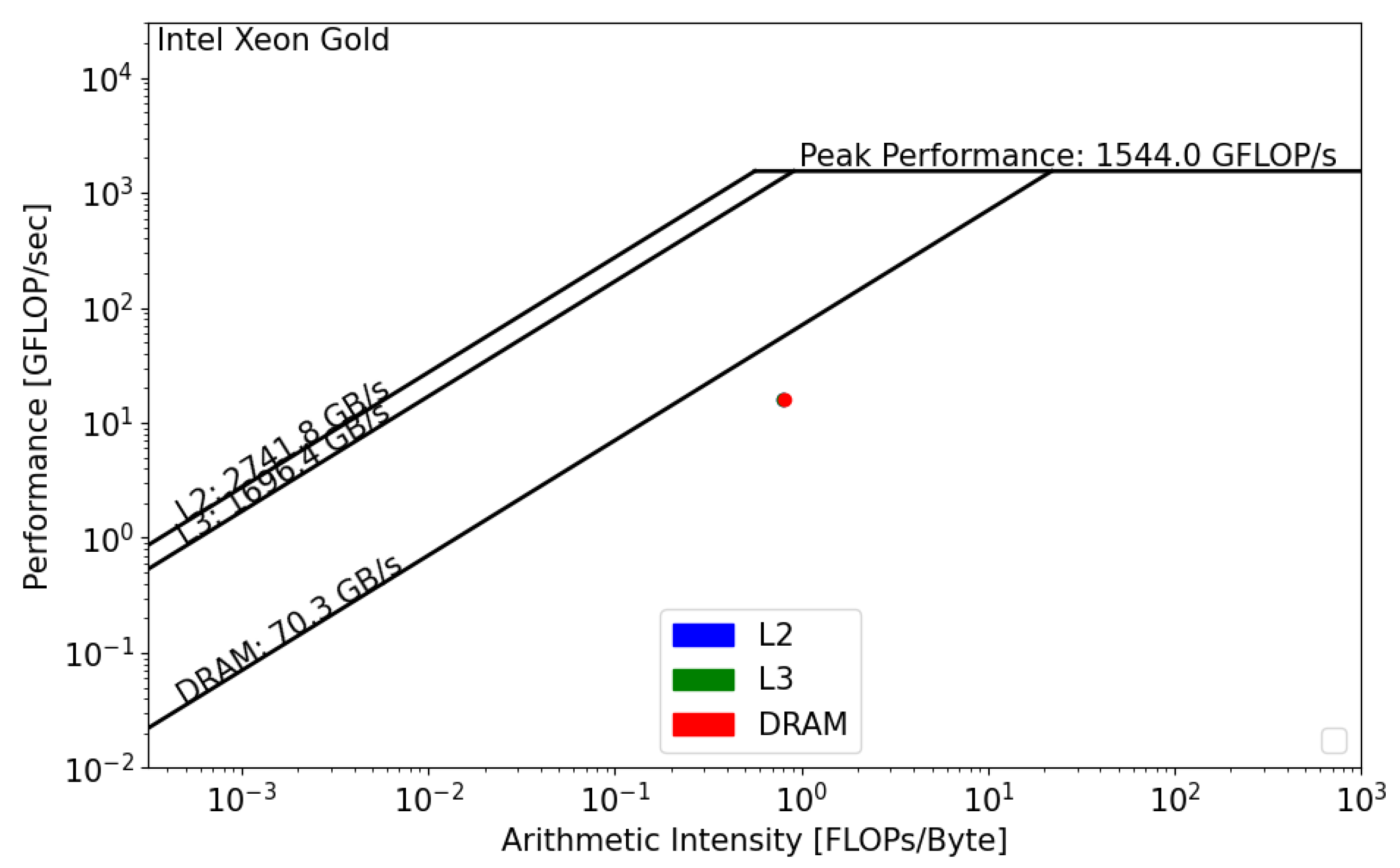
The CPU roofline models are presented below. We used dataset . The main difference between the two CPUs is the DRAM bandwidth. For the Intel Xeon processor, the memory bandwidth is equal to 70.3 GB/s, and, for the AMD EPYC processor, it is equal to 221.1 GB/s. Regarding the Floating Point performance, Intel Xeon has the lead with a = 1544 GFLOP/s. However, since the GRICS reconstruction relies on repeated FFT, the code will likely be impacted by the memory bandwidth, and efforts should be undertaken in this direction to optimize the code.
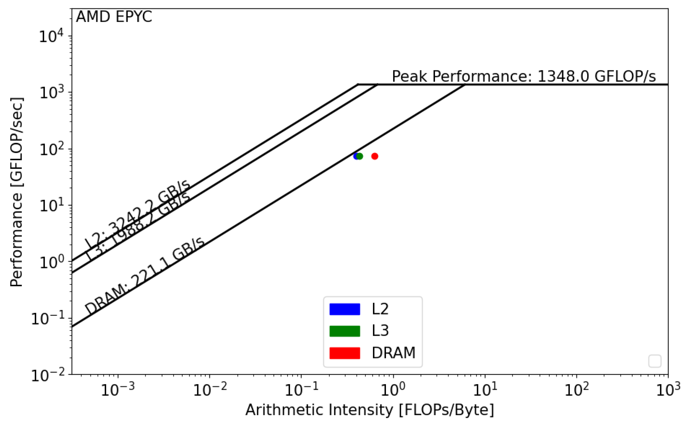
Intel SDE and Vtune report that the GRICS’s operational intensity is equal to FLOP/byte. AMDProf reports that FLOP/byte. Using Figure 8 and Figure 9, we can see that, in both architectures, the GRICS is memory bound. In Intel Xeon, the code is mainly limited by the low value of the DRAM bandwidth; its actual performance is equal to 16 GFLOP/s. is far from the theoretical bound for this value of operational intensity; a code that has a similar value of and that uses the micro-architecture of the processor in a better way can operate at a performance equal to 56 GFLOP/s. Using Equation (4), the code’s architectural efficiency on Xeon is 28%. On the AMD EPYC CPU, it performs better, with a performance equal to 80 GFLOP/s. In this architecture, the code benefits from the high value of the memory bandwidth, GB/s. Its architectural efficiency on EPYC is 52%. Moreover, the figures show that , which means that there is poor data reuse; once the data are loaded from the main memory, they are not reused while being in caches and instead evicted. This is not the case regarding the AMD EPYC CPU, where is greater than and , which means that the data are being reused once they are loaded from DRAM.
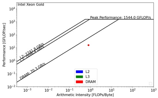
Figure 8.
Roofline analysis of GRICS on Intel Xeon Gold.
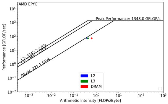
Figure 9.
Roofline analysis of GRICS on AMD EPYC.
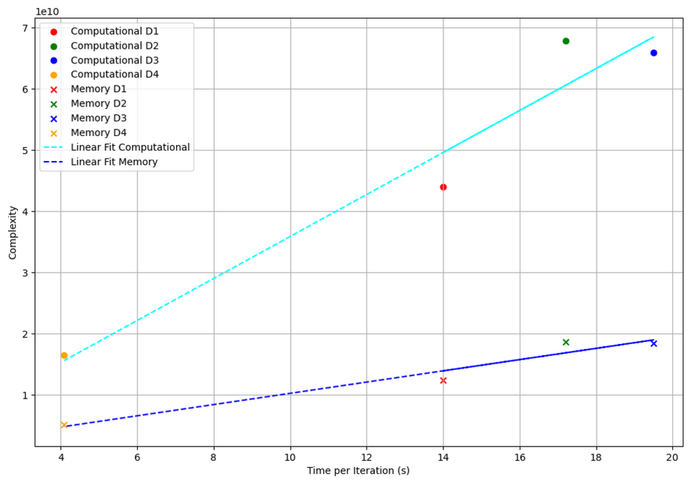
Figure 10 presents the computational and memory complexity of Algorithm 2 as a function of the elapsed time per iteration on the AMD EPYC CPU. The complexities are computed using Equations (7) and (8). Datasets and align closely with the predicted trend, both for memory and computation. lies above the linear fitting lines, suggesting lower computational and memory efficiency than expected. shows both good memory and computational efficiency, positioned below the fitting lines.
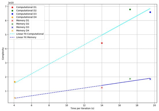
Figure 10.
Computational and memory complexity of the reconstruction kernel as a function of elapsed time per iteration (on AMD EPYC CPU). The cyan and blue dashed lines in the plot represent the linear regression fits for computational and memory complexities, respectively. Time per iteration refers to the elapsed time of the reconstruction kernel per conjugate gradient iteration.
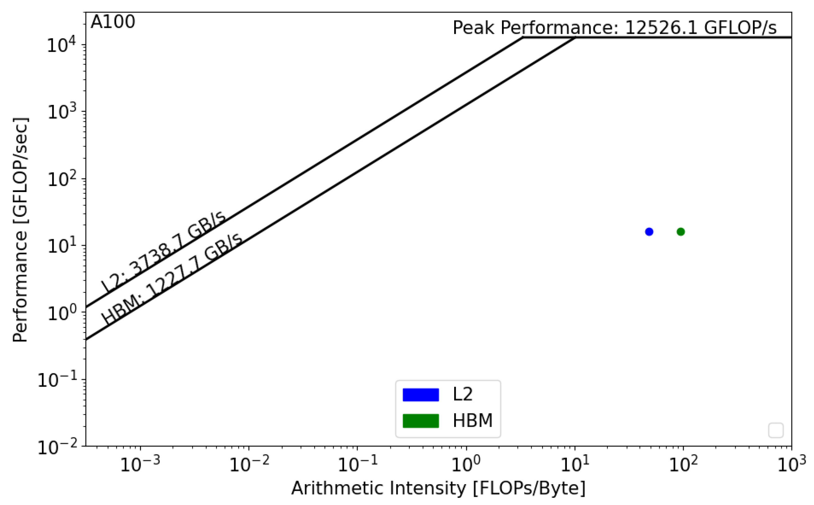
Figure 11 and Figure 12 present the GPU roofline models. In both architectures, the reconstruction kernel is compute bound. The kernel’s performance on RTX 5000 is equal to 5 GFLOP/s, while its performance on A100, , is equal to 16 GFLOP/s. In both cases, the actual performance is far from the roofline boundaries, which means that the actual implementation does not properly use the GPU architecture and that source-code modifications should be considered in order to achieve better performance. Moreover, we notice the absence of data reuse on Quadro RTX, , which means that there are repetitive calls to the main memory in order to satisfy the load and store operations. However, the data are being reused on A100, which reduces the latency and improves the overall performance of the kernel.
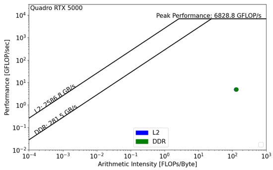
Figure 11.
Roofline analysis of on NVIDIA Quadro RTX 5000.
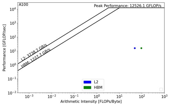
Figure 12.
Roofline analysis of on NVIDIA A100.
NVIDIA Nsight compute offers features to evaluate the achieved percentage of utilization of each hardware component with respect to the achieved maximum. In Figure 13, we compare these throughputs on the two devices.
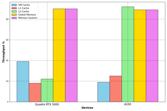
Figure 13.
Performance throughputs on RTX 5000 and A100. On GPUs, the main memory system is used optimally, and the achieved throughputs are 90% and 89% for RTX 5000 and A100, respectively. The first difference concerns the L2 cache throughput, 22% for RTX 5000 and 92% for A100. However, the main hardware limitation is the SM utilization; the throughputs are low on both architectures.
The A100 GPU has 40 MB of L2 cache, which is 10 times larger than Quadro’s L2 cache. The increase in the L2 cache size improves the performance of the workloads since larger portions of datasets can be cached and repeatedly accessed at a much higher speed than reading from and writing to HBM memory, especially the workloads that require a considerable memory bandwidth and memory traffic, which is the case for this kernel. Moreover, the main memory bandwidth is intensively used by the kernel on both architectures, while the SM throughput is low, which helps us in determining the kernel’s bottleneck on GPUs. The compute units are not optimally used; architecture optimization would also greatly improve the GPUs’ compute throughput regarding the Tensor and CUDA cores.
5.2. Optimization Results
In order to understand the impact of thread binding and affinity, we present the different elapsed times of GRICS with different configurations using only OpenMP. The elapsed time of the code is insensitive to the variable OMP_PLACES. Hence, we choose to bind the threads to hardware threads. However, the elapsed time is remarkably sensitive to the binding strategy.
- -
- OS OMP: Only OpenMP parallelization over the receiver coils is considered, with basic optimization flags and without thread binding. The GNU C++ compiler is considered.
- -
- Close OMP: The thread affinity is enabled with the close option.
- -
- Spread OMP: The thread affinity is enabled with the spread option. In the three cases, the compilation flags discussed in Section 4.4.1 are enabled.
Each OpenMP configuration for each dataset is executed five times; the reported time is the mean of the five experiments. Since we are the only user at the workstation while conducting the testing, the differences in the execution times between multiple runs (for a given binding strategy) are not significant: the standard deviations range from 0.30 s to 1.001 s. The thread binding and compilation flags do not impact the numerical accuracy and stability of the program since the number of conjugate gradient iterations remain the same with spread/close bindings: 4, 5, 4, and 11 iterations, respectively, for , and .
Moreover, we compute the Normalized Root Mean Square Error to prove that there is no image quality degradation with the proposed optimizations: , and stand, respectively, for the reconstructed images with the spread, close, and no binding options; we calculate max(NRMSE(), NRMSE(), and NRMSE()). These values are, respectively, equal to 4.67 , 5.95 , 4.89, and 2.40 for , and .
Thread binding and affinity decisions (spread or close) are architecture-dependent for the same program. Using Table 6, we can see that, on the AMD EPYC processor, the spread option enables a gain of 9–17% on the AMD EPYC CPU, while the close option degrades the performance compared to the OS allocation. On the Intel CPU, the code is much slower, and the close option yields better results compared to the spread binding. However, the OS thread allocation is more suitable to the GRICS on this architecture.
Table 6.
Elapsed time of GRICS with different OpenMP configurations on CPUs.
The roofline analysis and the performance of the GRICS’s OpenMP version prove that the EPYC CPU is more suitable for the code, notably in terms of its demanding data traffic. The high value of EPYC’s DRAM bandwidth accelerates the rate at which the data are transferred to the compute units and enables rapid execution. For these reasons, we decided to investigate the performance of the hybrid version only on the AMD EPYC CPU; the different execution times are presented in Figure 14.
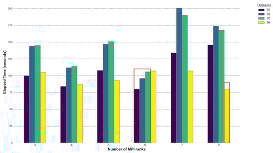
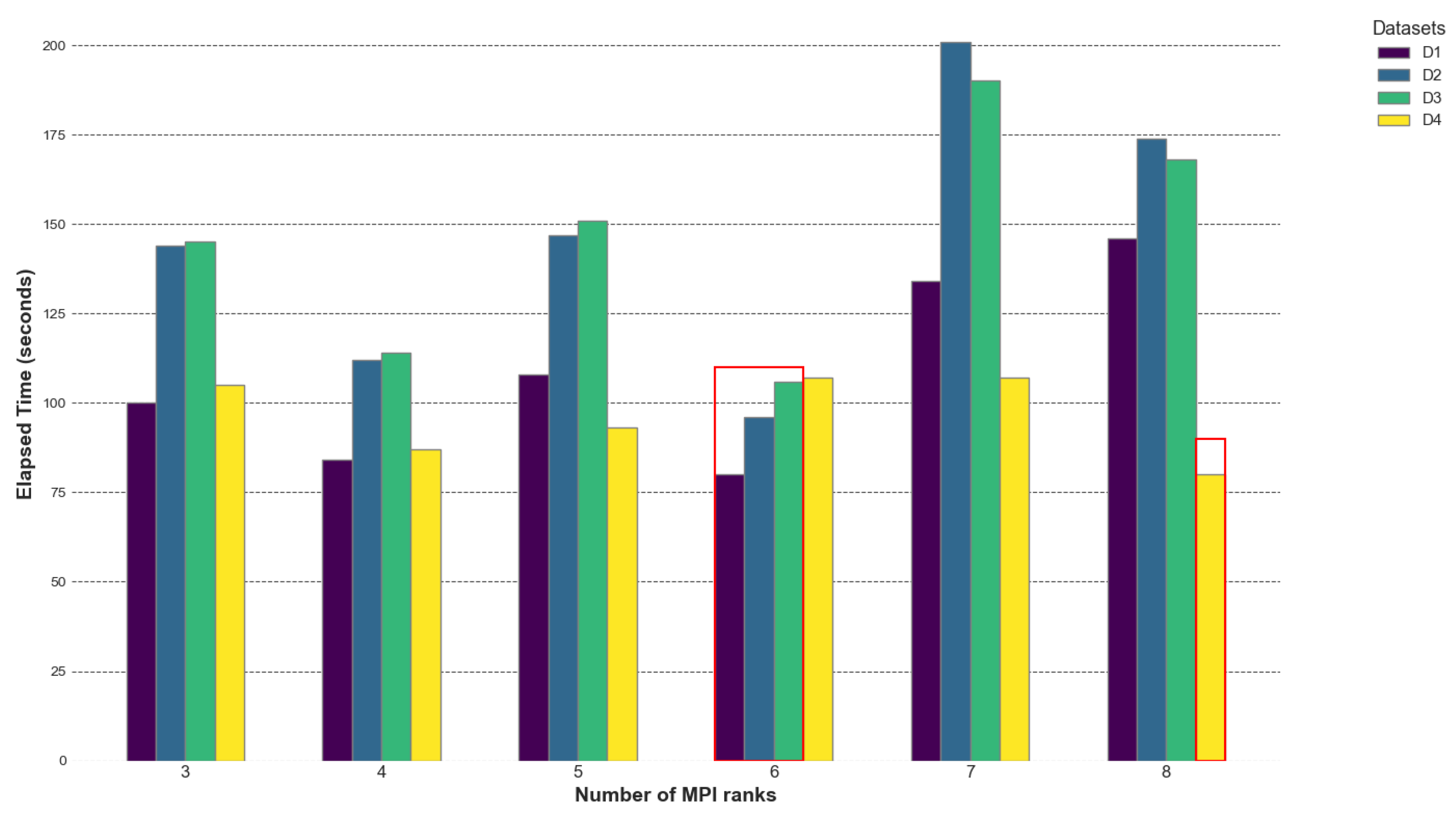
Figure 14.
Elapsed time of GRICS for different MPI processes on AMD EPYC; the number of OpenMP threads was fixed to 20. The reported times are the mean of 5 executions. The maximum standard deviations were 0.96, 0.14, 0.39, and 0.13 for , , , and , respectively. We highlighted the best times per dataset in red.
The GRICS’s hybrid implementation improves the overall performance in terms of elapsed time. The best performances are achieved when the number of MPI processes n divides the number of motions states ; for datasets , and , is equal to 12 and the minimal times are reported for . The best performance is achieved with ranks. For dataset with , the minimal elapsed time corresponds to the and processes. When the number of processes n divides the number of motion states evenly, it leads to better load balancing. Each process receives an equal share of the workload, minimizing idle times. The empirical data show that the elapsed time initially decreases with increasing processes (up to a certain point) and then starts increasing. More processes may increase the number of communications required, leading to higher network traffic and contention. For the OpenMP parallelization of the loop over the coils, choosing a number of threads m such that m divides does not greatly improve the overall performance; the set of threads m when provides approximately the same result. A small improvement is noticed when . The best MPI OpenMP settings are and for all the datasets.
Finally, we present in Table 7 a performance-based comparison between the CPUs and GPUs for the reconstruction kernel. The reported times correspond to the best parallelization strategy for each device; we use dataset . There is no significant difference between the MRI images from the CPUs and GPUs. Setting and as the reconstructed images using the CPU and GPU, respectively, the Normalized Root Mean Square Error of the two images, NRMSE, is equal to , which is less than the tolerance of the reconstruction solver ().
Table 7.
Performance comparison of CPU/GPU. On CPUs, P stands for the performance of GRICS, while it stands for the reconstruction kernel’s performance on GPUs. However, both performances can be compared since the reconstruction kernel represents 70–80% of the GRICS’s elapsed time. The kernel’s performance on the CPU would be close to the GRICS’s performance on CPU. T is the elapsed time of the kernel.
From an architectural perspective, the kernel and GRICS operate well on an AMD EPYC CPU. The roofline analysis on the A100 GPU and the kernel’s elapsed time on this architecture provide us insights about the possible benefits of a full GPU implementation of the GRICS. Even if the actual one is not “GPU architecture aware”, its result is promising. On Quadro RTX5000, the code is slower; Nsight compute reports that L2–DDR data transfer is one of the bottlenecks on this GPU. However, the main hardware limitation on GPUs is the SM’s poor utilization. Both devices offer sophisticated compute capabilities with Tensor cores and CUDA cores, but the actual implementation is not adapted to using the GPU architecture properly, which is why the overall performance values, and , are low compared to . On the Intel Xeon Gold CPU, the code is mainly limited by the low value of memory bandwidth, absence of data reuse, and absence of vectorization.
6. Discussion
Using the proposed optimizations renders GRICS reconstruction available at the MRI console within an acceptable delay (80–102 s depending on the dataset), even in the case of very high-resolution 3D images. This delay is smaller than the typical acquisition time for one sequence of the examination. This is important for clinical use as the radiologist needs to visualize the images shortly after scanning, evaluate whether the image quality is sufficient for diagnostic use, and decide whether the patient can be released from the scanner. The optimal processor architecture is algorithm-dependent, and the roofline model is a visual model that helps in evaluating the software–hardware interaction. It is difficult to suggest a parallelization strategy that would be beneficial to every architecture or to confirm that an optimization pattern would improve the performance on multiple architectures. However, in this work, we presented steps to follow in order to evaluate the actual performance of a program, and ways to improve it with no source-code modification, by establishing the roofline model of the considered workstation using performance profiling tools to generate the operational intensity of the code and performing a roofline analysis to capture the hardware limitations and bottlenecks. In this work, we determined the main hardware limitations of the iterative MRI reconstruction algorithms, which are not straightforward to estimate, depending on the workstation (CPUs or GPUs).
For the CPU optimizations, we suggested to identify the appropriate compilation flags for the architecture, to test several binding strategies for the OpenMP parallelization, and to select the optimal number of MPI ranks to minimize the communication overhead and ensure effective parallelization.
We have shown that, without any code modification, using thread binding and affinity enables gains of 11%, 12%, 9%, and 17% for , , and , respectively, with only OpenMP on AMD EPYC. The GRICS’s architectural efficiency on this CPU is equal to 52%. However, the OS OpenMP affinity provides better results when it comes to Intel Xeon compared to the and options. On this CPU, the code’s architectural efficiency is 28%.
The optimal MPI and OpenMP combination yields gains of 62%, 65%, 68%, and 62% for , , and , respectively, on AMD EPYC. These gains are computed relative to the OS OpenMP elapsed time for each dataset. The reconstruction kernel’s elapsed time on the A100 GPU was the lowest, even if the roofline analysis pointed out that the GPU architecture is not optimally used. A low execution time does not guarantee an optimal GPU utilization. Figure 13 shows that the GPU memory bandwidth is used efficiently. However, the program is not fully utilizing the GPU’s available cores, leading to a suboptimal performance. For instance, using only a fraction of the available cores will leave the rest of the GPU’s resources idle (low SM throughput on both devices) and lead to an imbalanced workload among the threads. Optimal GPU utilization requires a program to effectively leverage the parallelism, memory bandwidth, load balancing, and efficient memory access patterns. Therefore, even with a low execution time, the program may still be far from making the best use of the GPU’s capabilities. We acknowledge that the GPU part of the study is preliminary and aimed at providing initial insights into the performance benefits of GPUs for our specific application. The future work will include a CUDA implementation of the reconstruction kernel (Algorithm 2), taking into account the results of the roofline model on GPUs.
In Ref. [41], Driscoll introduced several HPC techniques for computational image reconstruction with specific applications in the MRI field. He presented an architectural efficiency (peak percentage) comparison of the non-Cartesian SENSE normal operator across different computing platforms. The operator achieved peak percentages of 39% and 10%, respectively, on the Intel Xeon E5-2698 CPU and Intel Xeon Phi 7250 KNL processor. The GRICS method achieved a superior architectural efficiency on the AMD EPYC CPU and a better peak percentage on the Intel Xeon CPU compared to the Intel Xeon E5-2698 CPU. We recall that, since the GRICS is memory bound on a CPU, the peak percentage is computed relative to the memory performance for the GRICS’s operational intensity value rather than the peak floating point performance.
The proposed performance study and optimizations are not limited to GRICS. It is completely possible to follow the same steps in order to evaluate other computationally intensive MRI motion-compensated reconstruction codes that share the same bottleneck code as that described in Algorithm 2 and are applied by many authors [11].
The performance study does not confirm that the AMD EPYC CPU will outperform every Intel CPU in resolving motion-compensated reconstruction problems. We have chosen a specific Intel processor with a specific memory bandwidth and compute performance. Our study showed that, on CPUs, GRICS will perform better on an architecture that offers high memory and cache bandwidths. For example, our work can lead us to propose a suitable Intel architecture for GRICS, which is the Intel Xeon Phi 7235 Processor; the GRICS would benefit from Xeon’s Phi Multi-Channel DRAM (MCDRAM); the multi-channel aspect is the key to more bandwidth. Affording more channels regarding the DRAM leads to more simultaneous accesses, thus improving the bandwidth. Intel Xeon Phi processors include an on-package MCDRAM to increase the bandwidth available to a program at the same level in the memory hierarchy as the DDR memory but with higher bandwidth (High-Bandwidth Memory). The MCDRAM can serve as a high-bandwidth cache for DDR memory. It has a 450 GB/s bandwidth, and, assuming GRICS bottlenecks and hotspots, we would receive a performance improvement on this architecture. In [42], the authors proved that MCDRAM integration offers considerable speedup of the matrix–vector operations (the same type of operations in the GRICS) in Multilayer Perceptron and Recurrent Neural Networks compared to Tensor Product Units (TPUs) and an NVIDIA P4 GPU. A more recent choice would be the Intel Xeon Platinum 8380 processor, suitable for data-intensive workloads. With support for eight channels of DDR4-3200, it offers a maximum memory bandwidth of 204.8 GB/s, making it appropriate for memory-intensive applications. Moreover, Intel DL Boost and AVX-512 provide significant performance improvements for HPC applications. It is crucial to deeply understand the hardware limitations and bottlenecks of the application in order to suggest a suitable architecture.
7. Conclusions
For clinical use, the optimization of reconstruction in MRI is an important subject. We evaluated the performance of motion-compensated reconstruction algorithms using the GRICS code as an example, and we determined their main bottlenecks and hotspots. Using the roofline model, we have shown that the memory bandwidth is the main hotspot for this class of advanced MRI reconstruction on CPUs. The thread binding strategy resulted in up to a 17% performance gain when considering only OpenMP parallelization. The architectural efficiency of the program was 28% on Intel Xeon Gold and 52% on AMD EPYC. On the GPU devices, the reconstruction kernel was limited by the computational performance and compute throughput, indicating that the actual implementation does not fully exploit the GPU computational capabilities. Efforts should be directed towards maximizing the workload distribution among threads. However, the roofline analysis of the reconstruction kernel on the A100 GPU, where host–device transfer was not an issue, highlighted that a native C++ GPU implementation of this program, using for example CUDA, could leverage the hardware capabilities more efficiently and achieve a better performance. As a result of the findings, the next step involves implementing a native C++ version of the reconstruction kernel using CUDA, starting with the micro-kernels of Algorithm 2, particularly the sparse matrix vector product, the 1D and 2D FFT, and the element-wise matrix product.
Supplementary Materials
The following supporting information can be downloaded at https://www.mdpi.com/article/10.3390/app14219663/s1, Table S1: Performance Benchmarking of 3D FFT on the computing platforms.
Author Contributions
Conceptualization, M.A.Z., P.-A.V. and F.O.; methodology, M.A.Z., K.I., P.-A.V. and F.O.; software, M.A.Z., K.I., P.-A.V. and F.O.; validation, M.A.Z. and F.O.; formal analysis, M.A.Z., P.-A.V. and F.O.; investigation, M.A.Z., K.I., P.-A.V. and F.O.; resources, M.A.Z., K.I., P.-A.V. and F.O.; data curation, M.A.Z., K.I., P.-A.V. and F.O.; writing—original draft preparation, M.A.Z.; writing—review and editing, K.I., P.-A.V. and F.O.; visualization, M.A.Z., K.I., P.-A.V. and F.O.; supervision, P.-A.V. and F.O.; project administration, P.-A.V. and F.O. All authors have read and agreed to the published version of the manuscript.
Funding
MOSAR project (ANR-21-CE19-0028), CPER IT2MP, FEDER (European Regional Development Fund).
Institutional Review Board Statement
The study was conducted in accordance with the ethical principles outlined in the Declaration of Helsinki (1975, revised 2013) and was approved by the ethics committee (approval number: [CPP EST-III, 08.10.01]) under the protocol “METHODO” (ClinicalTrials.gov Identifier: NCT02887053). All participants provided written informed consent prior to their inclusion in the study.
Informed Consent Statement
Written informed consent has been obtained from the patients involved in this study.
Data Availability Statement
The original contributions presented in the study are included in the article, further inquiries can be directed to the corresponding author.
Acknowledgments
The authors would like to thank Vadim Karpusenko, from IonQ company, Christophe Picard, from Grenoble INP-Ensimag, Université Grenoble Alpes, and Damien Husson, from CIC-IT Nancy, for their valuable advice and suggestions.
Conflicts of Interest
The authors declare no conflicts of interest.
Abbreviations
| MRI | Magnetic Resonance Imaging |
| CPU | Central Processing Unit |
| GPU | Graphics Processing Unit |
| HPC | High-Performance Computing |
| FFT | Fast Fourier Transform |
| MPRAGE | Magnetization-Prepared Rapid Gradient Echo |
| OpenMP | Open Multi-Processing |
| MPI | Message Passing Interface |
| GRICS | The Generalized Reconstruction by Inversion of Coupled Systems |
| CUDA | Compute Unified Device Architecture |
| FLOPs | Floating Point Operations |
References
- Cabezas, V.; Püschel, M. Extending the roofline model: Bottleneck analysis with microarchitectural constraints. In Proceedings of the 2014 IEEE International Symposium on Workload Characterization (IISWC), Raleigh, NC, USA, 26–28 October 2014; pp. 222–231. [Google Scholar] [CrossRef]
- Eyerman, S.; Heirman, W.; Hur, I. DRAM Bandwidth and Latency Stacks: Visualizing DRAM Bottlenecks. In Proceedings of the 2022 IEEE International Symposium on Performance Analysis of Systems and Software (ISPASS), Singapore, 22–24 May 2022; pp. 322–331. [Google Scholar] [CrossRef]
- Denoyelle, N.; Goglin, B.; Jeannot, E.; Ropars, T. Data and Thread Placement in NUMA Architectures: A Statistical Learning Approach. In Proceedings of the 48th International Conference on Parallel Processing, ICPP ’19, Kyoto, Japan, 5–8 August 2019; pp. 1–10. [Google Scholar] [CrossRef]
- Williams, S.; Waterman, A.; Patterson, D. Roofline: An insightful visual performance model for multicore architectures. Commun. ACM 2009, 52, 65–76. [Google Scholar] [CrossRef]
- Schaetz, S.; Voit, D.; Frahm, J.; Uecker, M. Accelerated Computing in Magnetic Resonance Imaging: Real-Time Imaging Using Nonlinear Inverse Reconstruction. Comput. Math. Methods Med. 2017, 2017, e3527269. [Google Scholar] [CrossRef] [PubMed]
- Hansen, M.; Atkinson, D.; Sorensen, T. Cartesian SENSE and k-t SENSE reconstruction using commodity graphics hardware. Magn. Reson. Med. 2008, 59, 463–468. [Google Scholar] [CrossRef] [PubMed]
- Sorensen, T.; Schaeffter, T.; Noe, K.; Hansen, M. Accelerating the Nonequispaced Fast Fourier Transform on Commodity Graphics Hardware. IEEE Trans. Med. Imaging 2008, 27, 538–547. [Google Scholar] [CrossRef]
- Murphy, M.; Alley, M.; Demmel, J.; Keutzer, K.; Vasanawala, S.; Lustig, M. Fast ℓ1-SPIRiT Compressed Sensing Parallel Imaging MRI: Scalable Parallel Implementation and Clinically Feasible Runtime. IEEE Trans. Med. Imaging 2012, 31, 1250–1262. [Google Scholar] [CrossRef]
- Odille, F.; Cîndea, N.; Mandry, D.; Pasquier, C.; Vuissoz, P.A.; Felblinger, J. Generalized MRI reconstruction including elastic physiological motion and coil sensitivity encoding. Magn. Reson. Med. 2008, 59, 1401–1411. [Google Scholar] [CrossRef]
- Batchelor, P.; Atkinson, D.; Irarrazaval, P.; Hill, D.; Hajnal, J.; Larkman, D. Matrix description of general motion correction applied to multishot images. Magn. Reson. Med. 2005, 54, 1273–1280. [Google Scholar] [CrossRef]
- Odille, F. Chapter 13—Motion-Corrected Reconstruction. In Advances in Magnetic Resonance Technology and Applications; Magnetic Resonance Image Reconstruction; Akçakaya, M., Doneva, M., Prieto, C., Eds.; Academic Press: Cambridge, MA, USA, 2022; Volume 7, pp. 355–389. [Google Scholar] [CrossRef]
- Odille, F.; Vuissoz, P.A.; Marie, P.Y.; Felblinger, J. Generalized Reconstruction by Inversion of Coupled Systems (GRICS) applied to free-breathing MRI. Magn. Reson. Med. 2008, 60, 146–157. [Google Scholar] [CrossRef]
- Odille, F.; Menini, M.; Escanyé, J.M.; Vuissoz, P.A.; Marie, P.Y.; Beaumont, M. Joint Reconstruction of Multiple Images and Motion in MRI: Application to Free-Breathing Myocardial T_2 Quantification. IEEE Trans. Med. Imaging 2016, 35, 197–207. [Google Scholar] [CrossRef]
- Cordero-Grande, L.; Ferrazzi, G.; Teixeira, R.; O’Muircheartaigh, J.; Price, A.; Hajnal, J. Motion-corrected MRI with DISORDER: Distributed and incoherent sample orders for reconstruction deblurring using encoding redundancy. Magn. Reson. Med. 2020, 84, 713–726. [Google Scholar] [CrossRef]
- Cordero-Grande, L.; Teixeira, R.; Hughes, E.; Hutter, J.; Price, A.; Hajnal, J. Sensitivity Encoding for Aligned Multishot Magnetic Resonance Reconstruction. IEEE Trans. Comput. Imaging 2016, 2, 266–280. [Google Scholar] [CrossRef]
- Küstner, T.; Pan, J.; Qi, H.; Cruz, G.; Gilliam, C.; Blu, T.; Prieto, C. LAPNet: Non-rigid registration derived in k-space for magnetic resonance imaging. IEEE Trans. Med. Imaging 2021, 40, 3686–3697. [Google Scholar] [CrossRef] [PubMed]
- Balakrishnan, G.; Zhao, A.; Sabuncu, M.R.; Guttag, J.; Dalca, A.V. VoxelMorph: A learning framework for deformable medical image registration. IEEE Trans. Med. Imaging 2019, 38, 1788–1800. [Google Scholar] [CrossRef] [PubMed]
- Pan, J.; Rueckert, D.; Küstner, T.; Hammernik, K. Learning-based and unrolled motion-compensated reconstruction for cardiac MR CINE imaging. In Proceedings of the International Conference on Medical Image Computing and Computer-Assisted Intervention, Singapore, 18–22 September 2022; Springer: Cham, Switzerland, 2022; pp. 686–696. [Google Scholar] [CrossRef]
- Huttinga, N.R.; Van den Berg, C.A.; Luijten, P.R.; Sbrizzi, A. MR-MOTUS: Model-based non-rigid motion estimation for MR-guided radiotherapy using a reference image and minimal k-space data. Phys. Med. Biol. 2020, 65, 015004. [Google Scholar] [CrossRef] [PubMed]
- Chen, P.; Wahib, M.; Wang, X.; Takizawa, S.; Hirofuchi, T.; Ogawa, H.; Matsuoka, S. Performance Portable Back-projection Algorithms on CPUs: Agnostic Data Locality and Vectorization Optimizations. In Proceedings of the ACM International Conference on Supercomputing, New York, NY, USA, 14–17 June 2021; pp. 316–328. [Google Scholar] [CrossRef]
- Roujol, S.; de Senneville, B.; Vahala, E.; Sørensen, T.; Moonen, C.; Ries, M. Online real-time reconstruction of adaptive TSENSE with commodity CPU/GPU hardware. Magn. Reson. Med. 2009, 62, 1658–1664. [Google Scholar] [CrossRef]
- Inam, O.; Qureshi, M.; Laraib, Z.; Akram, H.; Omer, H. GPU accelerated Cartesian GRAPPA reconstruction using CUDA. J. Magn. Reson. 2022, 337, 107175. [Google Scholar] [CrossRef]
- Wang, H.; Peng, H.; Chang, Y.; Liang, D. A survey of GPU-based acceleration techniques in MRI reconstructions. Quant. Imaging Med. Surg. 2018, 8, 196–208. [Google Scholar] [CrossRef]
- Frigo, M.; Johnson, S. The Fastest Fourier Transform in the West; Technical Report MIT-LCS-TR-728; Massachusetts Institute of Technology: Cambridge, MA, USA, 1993. [Google Scholar]
- Blanchet, G.; Moisan, L. An explicit sharpness index related to global phase coherence. In Proceedings of the International Conference on Acoustics, Speech and Signal Processing (ICASSP), Kyoto, Japan, 25–30 March 2012; pp. 1065–1068. [Google Scholar] [CrossRef]
- Hager, G.; Wellein, G. Introduction to High Performance Computing for Scientists and Engineers; CRC Press: Boca Raton, FL, USA, 2010. [Google Scholar] [CrossRef]
- Yang, C.; Wang, Y.; Kurth, T.; Farrell, S.; Williams, S. Hierarchical Roofline Performance Analysis for Deep Learning Applications. In Proceedings of the Lecture Notes in Computer Science, Krakow, Poland, 16–18 June 2021; Volume 284, pp. 473–491. [Google Scholar] [CrossRef]
- Yang, C. Hierarchical Roofline analysis for GPUs: Accelerating performance optimization for the NERSC-9 Perlmutter system. In Concurrency and Computation: Practice and Experience; Wiley: Hoboken, NJ, USA, 2020. [Google Scholar] [CrossRef]
- Cook, S. CUDA Programming: A Developer’s Guide to Parallel Computing with GPUs, 1st ed.; Morgan Kaufmann Publishers Inc.: San Francisco, CA, USA, 2012. [Google Scholar]
- blitzpp. blitz. Available online: https://github.com/blitzpp/blitz (accessed on 6 May 2024).
- Agullo, E.; Demmel, J.; Dongarra, J.; Hadri, B.; Kurzak, J.; Langou, J.; Ltaief, H.; Luszczek, P.; Tomov, S. Numerical linear algebra on emerging architectures: The PLASMA and MAGMA projects. J. Phys. Conf. Ser. 2009, 180, 012037. [Google Scholar] [CrossRef]
- Isaieva, K.; Meullenet, C.; Vuissoz, P.-A.; Fauvel, M.; Nohava, L.; Laistler, E.; Zeroual, M.A.; Henrot, P.; Felblinger, J.; Odille, F. Feasibility of online non-rigid motion correction for high-resolution supine breast MRI. Magn. Reson. Med. 2023, 90, 2130–2143. [Google Scholar] [CrossRef]
- GitHub-Ebugger. Empirical Roofline Toolkit. Available online: https://github.com/ebugger/Empirical-Roofline-Toolkit (accessed on 3 June 2024).
- Example Scripts for Plotting Roofline. Available online: https://github.com/cyanguwa/nersc-roofline (accessed on 4 June 2024).
- Intel. Intel VTune. Available online: https://www.intel.com/content/www/us/en/developer/tools/oneapi/vtune-profiler.html#gs.yebp2q (accessed on 10 June 2024).
- Intel. Intel® Software Development Emulator. Available online: https://www.intel.com/content/www/us/en/developer/articles/tool/software-development-emulator.html (accessed on 10 June 2024).
- Yang, C. Hierarchical Roofline Analysis: How to Collect Data using Performance Tools on Intel CPUs and NVIDIA GPUs. arXiv 2020, arXiv:2009.02449. [Google Scholar]
- AMD uProf. Available online: https://www.amd.com/en/developer/uprof.html (accessed on 17 June 2024).
- Nsight Compute. Available online: https://docs.nvidia.com/nsight-compute/NsightCompute/ (accessed on 1 July 2024).
- Halbiniak, K.; Wyrzykowski, R.; Szustak, L.; Kulawik, A.; Meyer, N.; Gepner, P. Performance exploration of various C/C++ compilers for AMD EPYC processors in numerical modeling of solidification. Adv. Eng. Softw. 2022, 166, 103078. [Google Scholar] [CrossRef]
- Driscoll, M. Domain-Specific Techniques for High-Performance Computational Image Reconstruction. Ph.D. Thesis, University of California, Berkeley, CA, USA, 2018. [Google Scholar]
- Shin, H.; Kim, D.; Park, E.; Park, S.; Park, Y.; Yoo, S. McDRAM: Low Latency and Energy-Efficient Matrix Computations in DRAM. IEEE Trans.-Comput.-Aided Des. Integr. Circuits Syst. 2018, 37, 2613–2622. [Google Scholar] [CrossRef]


Disclaimer/Publisher’s Note: The statements, opinions and data contained in all publications are solely those of the individual author(s) and contributor(s) and not of MDPI and/or the editor(s). MDPI and/or the editor(s) disclaim responsibility for any injury to people or property resulting from any ideas, methods, instructions or products referred to in the content. |
© 2024 by the authors. Licensee MDPI, Basel, Switzerland. This article is an open access article distributed under the terms and conditions of the Creative Commons Attribution (CC BY) license (https://creativecommons.org/licenses/by/4.0/).