Intelligent Diagnosis of Bearing Failures Based on Recurrence Quantification and Energy Difference

Abstract

Bearing health is key for maintaining good performance and safety in rotating machinery. As the diagnosis of mechanical faults develops toward intelligence and automation, accurate and systematic fault diagnosis algorithms are imperative. Focusing on the diagnosis of rolling bearing failures, this study utilizes a sliding time window to extract essential data segments. A series of signal processing techniques, including filtering, amplitude–frequency analysis, Hilbert envelope analysis, and energy analysis, is applied to establish a comprehensive dataset. For extraction of the hidden properties of the data, the recurrence quantity spectrum is defined for the input of the neural network. The goal is to obtain a cleaner dataset with enhanced features. A convolution neural network is constructed. Different activation functions in the activation layer are compared for better fault diagnosis algorithms. The established feature matrices are specifically defined to accurately identify the subtlest defects of bearings, thereby facilitating early detection. The proposed procedure distinguishes various fault modes. As for the multidimensional complexities of fault signals, this study carries out a comprehensive comparison of energies, recurrence quantification, and amplitude–frequency characteristics of bearing fault detection to assess the accuracy, computational efficiency, and robustness of bearing fault diagnosis. The proposed method and bearing fault detection procedures have potential in practical applications.

1. Introduction

With the rapid advancement of modern industry and science technology, mechanical equipment is swiftly progressing toward high-speed intelligence, precision systematization, high-efficiency automation, and deep cleanliness. As the structural complexity of mechanical equipment increases and the interdependencies among its components become more intricate, the safe, stable, and efficient operation of this equipment is directly tied to corporate economic interests and production safety. Component failures can result in substantial financial losses and potentially severe consequences, including environmental pollution and personal injuries. Consequently, real-time monitoring and the fault diagnosis of mechanical equipment are critically important.

To improve fault diagnosis accuracy and understand fault reasons and types, many researchers have focused on this area. In 2009, Yang [1], from the University of Science and Technology of China, undertook a detailed study and analysis of the application of uncertainty theory in the field of mechanical fault diagnosis. He developed a probability inference methodology based on the connection tree algorithm and a consultation diagnostic fusion model grounded in Dempster–Shafer (D-S) evidence theory. These contributions provided targeted and effective solutions to address the uncertainties inherent in mechanical fault diagnosis. In 2013, Bruna et al. [2] introduced the first graph-based neural network, formally applying convolutional neural network (CNN) models to the analysis and modeling of graph-structured data and their practical applications. This work garnered significant attention in the fields of machine vision and pattern recognition. In 2016, Guo et al. [3] proposed a novel hierarchical learning rate adaptive deep convolutional neural network based on an improved algorithm and investigated its use for diagnosing bearing faults and determining their severity. In 2017, Zhang W. [4], from Harbin Institute of Technology, conducted a study utilizing convolutional neural networks (CNNs) in the context of specific electromechanical equipment fault diagnosis. He proposed an enhanced CNN framework, referred to as WDCNN, specifically tailored for fault diagnosis in the components of rotating mechanical systems. Through additional research and analysis, Zhang improved the adaptive batch normalization algorithm, substantially enhancing the load adaptability and noise resilience of the designed WDCNN model. In 2017, Li et al. [5] proposed a novel bearing fault diagnosis algorithm, IDSCNN, based on an ensemble of deep convolutional neural networks and an improved evidence fusion algorithm based on Dempster’s theory, which achieved better fault diagnosis performance than the existing machine learning approaches by fusing compensating or conflicting evidence from different models and sensors and adapting to different load conditions. In 2017, Yuan J. et al. [6] performed continuous wavelet transform (CWT) on the vibration signals of rolling bearings to obtain time–frequency diagrams of the fault data, which were visualized as grayscale images. After resizing the time–frequency diagrams to appropriate dimensions, they served as feature maps and were fed into a CNN classifier model, enabling the intelligent fault diagnosis of different modes of rolling bearings. In 2018, Qu J. et al. [7] proposed an “end-to-end” adaptive convolutional neural network (ACNN-FD) for fault diagnosis and monitoring. This approach constructs a deep network structure to enable the adaptive hierarchical extraction of features from raw vibration signals. In 2019, Xiao X. et al. [8] utilized a novel data preprocessing technique to transform raw time–domain signal data into two-dimensional grayscale images. By extracting features from the transformed images, they performed denoising on the fault dataset obtained through experimentation. They also adjusted the adaptive learning rate of the gradient descent algorithm in the convolutional neural network, effectively optimizing the algorithm’s performance. In 2019, Shao et al. [9] proposed a motor fault diagnosis method based on transfer learning. The main framework of the model consists of a VGG-16 model based on a convolutional neural network. This method first trains the fault diagnosis model on a dataset from the ImageNet image database, and then transfers the trained model. The specific method is to freeze the parameters of some layers of the network model after the pre-training is completed, then update some parameters for the motor dataset, and finally realize the rapid adaptation for the motor fault dataset. In 2023, Zhao et al. [10] introduced the hybrid information convolutional neural network (MIXCNN), which constitutes an efficient and compact framework for end-to-end fault diagnosis classification. A distinguishing characteristic of MIXCNN is its uniform output dimensionality across all convolutional layers, ensuring a consistent feature space representation. Zhao et al. [11] introduced an innovative fault diagnosis paradigm for rotor systems, anchored in an enhanced parallel convolutional neural network (PCNN) framework, complemented by an attention mechanism (termed AMPCNN). This structure leverages convolutional kernels of heterogeneous sizes across parallel pathways to process raw data inputs. Subsequently, a feature fusion phase integrates diverse feature maps to generate a more holistic representation, while the amalgamation of the attention mechanism facilitates reciprocal information exchange among parallel channels. When considering the idea of dynamics and stability in modeling a defect mechanical system, the Floquet theory and first-order approximation from the averaging method [12] can be referenced. For accurate bearing fault diagnosis, recurrence quantity spectrums are defined for a comprehensive dataset with enhanced features. Activation functions in the activation layer are optimized for better fault diagnosis. Feature matrices are specifically defined to identify the subtlest defects of bearings accurately. This research develops a more efficient fault detection procedure and algorithms that can serve as a universal model for practical bearing fault diagnosis in engineering.

Regarding the techniques of bearing fault diagnosis, the extraction of features from raw data is a critical component. This research commences by introducing the characteristic frequencies of rolling bearings alongside pertinent theoretical knowledge in Section 2. It explores feature extraction methods implemented through programming, elucidates the meaning and specific application of recurrence plots, and highlights the advantages of quantitative analysis using metrics in recurrence quantification analysis (RQA) in the subsections. The application of data washing techniques is provided in Section 3, accompanied by a bearing fault diagnosis technique based on machine learning. A comparison of the proposed procedures with other methods is given in Section 4. The last section summarizes this research.

2. Methodology

2.1. Characteristic Frequencies of Rolling Bearing

Rolling element bearings principally comprise four key components: the inner race, the outer race, the rolling elements, and the cage. During their operation, these bearings may exhibit various fault modes, each leading to distinct failure mechanisms. When any part of the bearing becomes locally damaged during operation, the machinery produces corresponding vibration frequencies, known as the fault characteristic frequencies of the rolling bearing.

When faults and defects occur in the bearings, unsmooth vibration and noise will happen. Chattering and rattled noise can be heard. Different components of bearings correspond to different characteristic frequencies during vibration and noise. The characteristic fault frequencies of the primary components of rolling bearings are outlined in

Table 1. Frequencies of rolling bearings.

Mechanical Motions	Frequencies
Rotation frequency of inner race	$f_{\mathrm{i}}={\displaystyle \frac{n}{60}}$
Slewing frequency of outer race	$f_{\mathrm{o}}=0$
Relative rotation frequency of inner and outer races	$f_{\mathrm{r}}=f_{\mathrm{i}}-f_{\mathrm{o}}$
Inner race fault	$f_{\mathrm{I}}={\displaystyle \frac{1}{2}}Z(1+{\displaystyle \frac{d}{D}}\cos \alpha )f_{\mathrm{r}}$
Outer race fault	$f_{\mathrm{O}}={\displaystyle \frac{1}{2}}Z(1-{\displaystyle \frac{d}{D}}\cos \alpha )f_{\mathrm{r}}$
Rolling element failure frequency	$f_{\mathrm{b}}={\displaystyle \frac{D}{2d}}(1-{\displaystyle \frac{d^2}{D^2}}{\cos }^2\alpha )f_{\mathrm{r}}$
Cage failure frequency	$f_{\mathrm{P}}={\displaystyle \frac{1}{2}}(1-{\displaystyle \frac{d}{D}}\cos \alpha )f_{\mathrm{r}}$

[13].

The variables are defined as follows: n denotes the rotational speed of the rolling bearing; Z denotes the number of rolling elements; d denotes the diameter of the rolling elements; D denotes the diameter of the circle on which the centers of the rolling elements lie; α denotes the contact angle of the rolling elements.

Sliding window techniques are indispensable tools for processing and analyzing time series data, serving as a common method for dataset augmentation. By effectively aggregating and analyzing data over a defined period, the window is incrementally moved over time, enabling the continuous analysis and processing of new datasets.

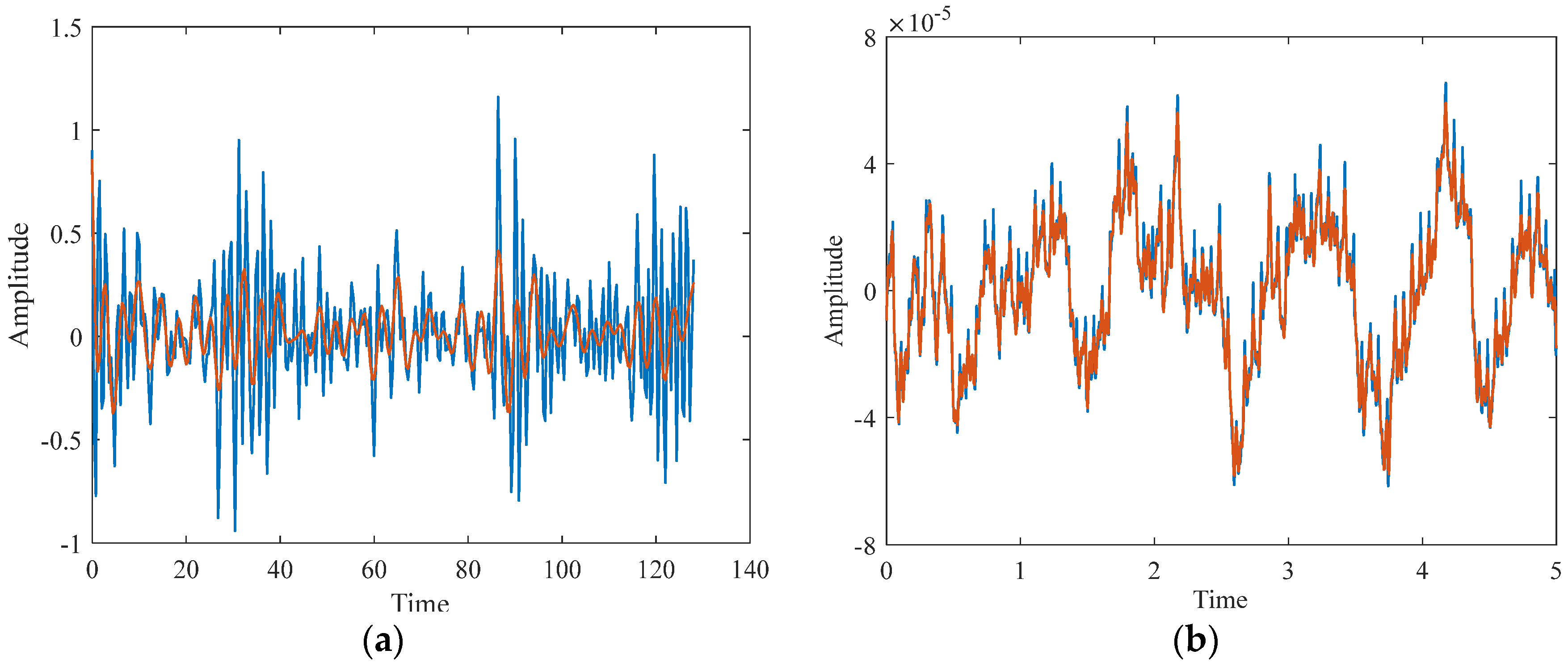
2.2. Hilbert Transformation

Hilbert transformation [14] is an effective analytical method for processing vibration and analytic signals. Considering a general continuous signal x(t) with its spectrum X(f), x(t) can be transformed as follows:

$$x\left(t\right)={\displaystyle {\int }_{-\infty }^{+\infty }X(f){\mathrm{e}}^{\mathrm{j}2\pi ft}\mathrm{d}f}$$

(1)

$$x(t)={\displaystyle {\int }_0^{+\infty }X\left(f\right){\mathrm{e}}^{\mathrm{j}2\pi ft}\mathrm{d}f}+{\displaystyle {\int }_{-\infty }^{0}X\left(f\right){\mathrm{e}}^{\mathrm{j}2\pi ft}\mathrm{d}f}$$

(2)

It can be deduced that

$$x(t)={\displaystyle {\int }_0^{+\infty }X\left(f\right){\mathrm{e}}^{\mathrm{j}2\pi ft}\mathrm{d}f}+{\displaystyle {\int }_0^{+\infty }X\left(f\right){\mathrm{e}}^{-\mathrm{j}2\pi ft}\mathrm{d}f}$$

(3)

Since $X\left(-f\right)=\overline{X(f)}$, the second term in the above equation can be changed to

$${\displaystyle {\int }_0^{+\infty }X\left(f\right){\mathrm{e}}^{-j2\pi ft}\mathrm{d}f}=\overline{{\displaystyle {\int }_0^{+\infty }X\left(f\right){\mathrm{e}}^{j2\pi ft}\mathrm{d}f}}$$

(4)

If the signal x(t) is represented as the real part of a complex signal consisting solely of positive frequency components, then x(t) can be transformed into the following form:

$$x\left(t\right)=\mathrm{Re}\left\{{\displaystyle {\int }_0^{+\infty }2X{\left(f\right)}^{{\mathrm{e}}^{\mathrm{j}2\pi ft}}\mathrm{d}f}\right\}$$

(5)

Then, the complex signal of x(t) can be denoted as q(t):

$$q\left(t\right)={\displaystyle {\int }_0^{+\infty }2X\left(f\right){\mathrm{e}}^{\mathrm{j}2\pi ft}\mathrm{d}f}$$

(6)

The spectrum of the complex signal q(t) is denoted as Q(f):

$$Q\left(f\right)=\left\{\begin{array}{cc}2X(f)& f>0\\ 0& f<0\end{array}\right.$$

(7)

The spectrum Q(f) can be obtained by filtering X(f). Assuming the spectrum of the filter is H₁(f), its computation is as follows:

$$H_1\left(f\right)=\left\{\begin{array}{cc}2& f>0\\ 0& f<0\end{array}\right.$$

(8)

$$Q(f)=H_1(f)X(f)$$

(9)

The time function h₁(t) corresponding to the spectrum H₁(f) is as follows:

$$h_1\left(t\right)=\delta \left(t\right)+\mathrm{j}{\displaystyle \frac{1}{\pi t}}$$

(10)

$$q\left(t\right)=h_1\left(t\right)\ast x\left(t\right)=\left(\delta \left(t\right)+\mathrm{j}{\displaystyle \frac{1}{\pi t}}\right)\ast x\left(t\right)$$

(11)

The expression $\tilde{x}\left(t\right)$ is referred to as the Hilbert transformation of the signal x(t):

$$\tilde{x}\left(t\right)={\displaystyle \frac{1}{\pi t}}\ast X\left(t\right)={\displaystyle \frac{1}{\pi }}{\displaystyle {\int }_{-\infty }^{+\infty }\frac{x\left(\tau \right)}{t-\tau }\mathrm{d}\tau }$$

(12)

It can be seen that a Hilbert transformation of a signal is equivalent to a filtering process, and the filtering factor h(t) is ${\displaystyle \frac{1}{\pi t}}$.

Appropriately applying Hilbert transformation enables the envelope analysis of fault signals, which in turn facilitates the calculation of the instantaneous phase and the examination of the instantaneous frequency. This approach provides valuable insights into the evolution of the entire fault signal.

2.3. Low-Pass Filtering and Band-Stop Filtering

Low-pass filtering, a widely used signal processing technique, attenuates high-frequency noise in signals and effectively smooths the target data. Band-stop filtering further reduces signals within a specific frequency range, thereby mitigating noise. In this paper, signals sliced by the sliding time window were filtered to effectively suppress noise interference. A comparison between the filtered signals and the original signals is illustrated in Figure 1.

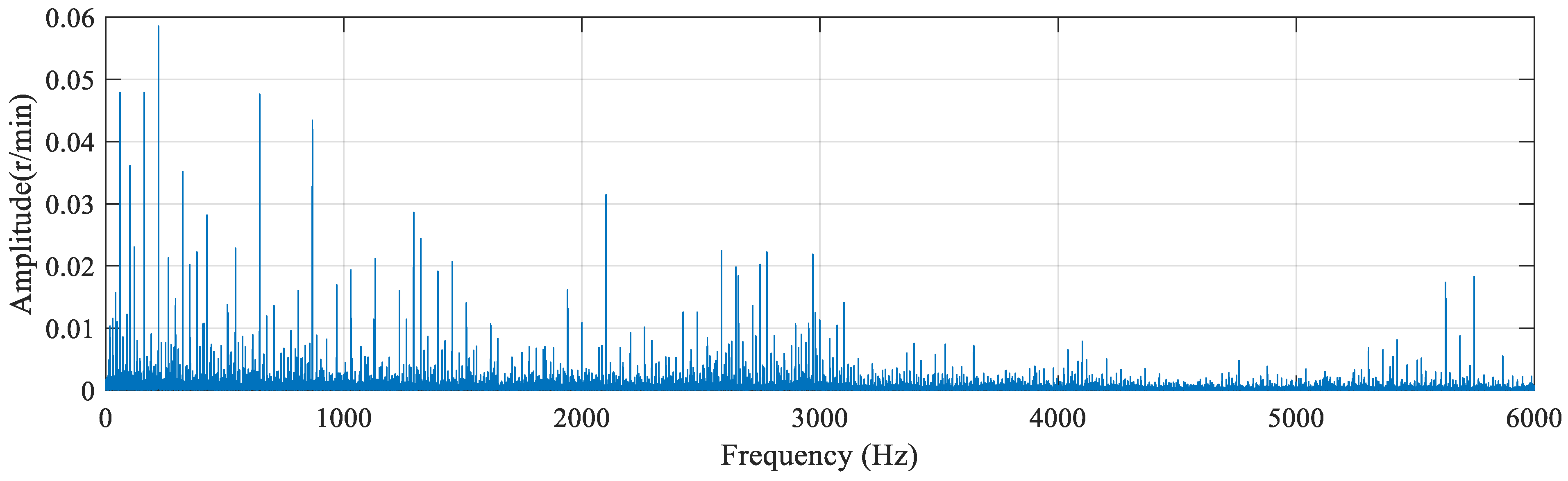
2.4. Power Spectral Density Analysis

The power spectral density (PSD) serves as an effective tool for assessing the distribution of energy in a signal across different frequencies. This method transforms time-domain signals into the frequency domain using Fourier transform and calculates the squared magnitude of each frequency component for subsequent analysis [15].

One of the fundamental results in Fourier analysis is Parseval’s theorem. This theorem asserts that the sum (or integral) of the square of a function, which represents its energy, is equivalent to the sum (or integral) of the square of its Fourier transform.

$${\displaystyle {\int }_{-\infty }^{+\infty }{\left|x\left(t\right)\right|}^2\mathrm{d}t}={\displaystyle {\int }_{-\infty }^{+\infty }{\left|X\left(f\right)\right|}^2\mathrm{d}f}$$

(13)

The equation for calculating the power spectral density is as follows:

$$P={\displaystyle {\int }_{-\infty }^{+\infty }{S}_x\left(f\right)\mathrm{d}f}$$

(14)

2.5. Recurrence Plots with the RQA Method

The definition of a recurrence plot is grounded in phase space reconstruction, reflecting the properties of the reconstructed attractor. Given the varying nature of vibration signals, the manifestation of their attractors differs, resulting in distinct structures in recurrence plots [16,17].

The algorithm for constructing a recurrence plot is outlined as follows:

$$\begin{array}{cc}{R}_{i,j}\left(\mathit{\epsilon }\right)=\Theta \left(\mathit{\epsilon }-\Vert {\overrightarrow{x}}_i-{\overrightarrow{x}}_j\Vert \right)& i,j=1,2,\cdots ,N\end{array}$$

(15)

where the matrix R_i,j denotes an N × N size matrix, with N corresponding to the number of elements in the state vector ${\overrightarrow{x}}_i$. The symbol ε signifies a predetermined threshold, and $\Theta (\cdot )$ represents the Heaviside step function ($\Theta (y)=0$, if $y\le 0$; $\Theta (y)=1$, if $y>1$). The norm $\Vert \cdot \Vert$ is employed to quantify the magnitude of vectors. Selecting an appropriate norm is essential for accurately constructing a recurrence plot.

For a given signal, the phase space can be reconstructed using a time-lag approach through the following steps. Subsequently, a recurrence plot for this signal can be constructed.

(1)

Assuming the initial signal is ${\overrightarrow{x}}_t$, it is reconstructed as $x_i$.

$$\begin{array}{cc}{x}_i=(u_i,u_{i+\tau },\cdots ,u_{i+(m-1)\tau })& i=1,2,\cdots ,N-(m-1)\tau \end{array}$$

(16)

An appropriate embedding dimension m and delay time τ are chosen based on the characteristics of the signal.

(2)

A suitable recurrence threshold and critical distance are determined to facilitate the subsequent matrix calculations.

(3)

The recurrence matrix is computed according to the specified equations.

(4)

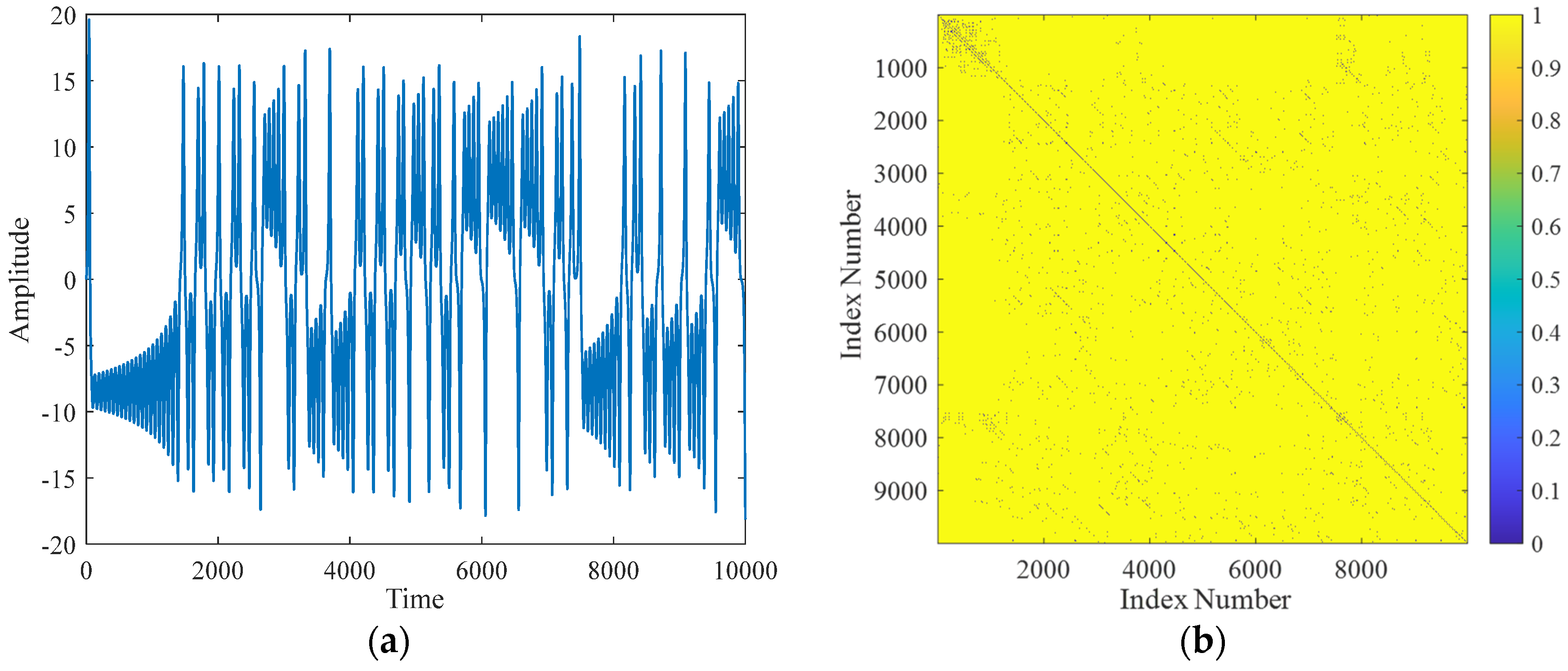
Based on the principles of recurrence plot construction, each point in the recurrence matrix is plotted along two axes to obtain the recurrence plot of the studied signal. Recurrence plots for the sine and Lorenz signals were generated using programming methods [16], as depicted in Figure 2 and Figure 3.

3. Experimental Implementation

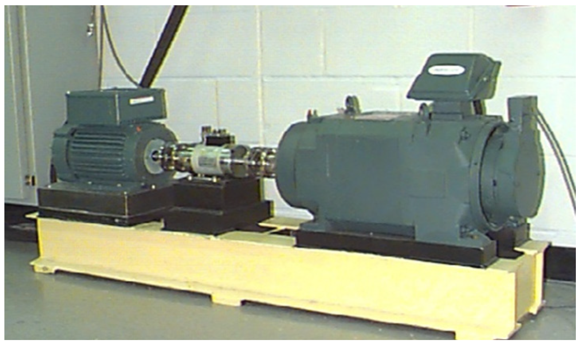
3.1. Datasets

The dataset used in this study was the publicly available rolling bearing fault dataset from Case Western Reserve University (CWRU) [18]. The experimental setup comprised a 1.5 kW motor, torque sensors, and a power meter, as depicted in Figure 4. The data used here were from the drive end bearings, which were double-sealed deep groove ball bearings (model 6205) manufactured by SKF. The sampling frequency for the experiments was 12 kHz. Three types of faults were identified in the bearings: inner race faults, outer race faults, and rolling element faults. Including the normal data, there were four types of experimental data in total. For the inner race faults, outer race faults, and rolling element faults, eight related data files were selected for each, and four data files were selected for the normal data for the subsequent fault extraction and training and testing.

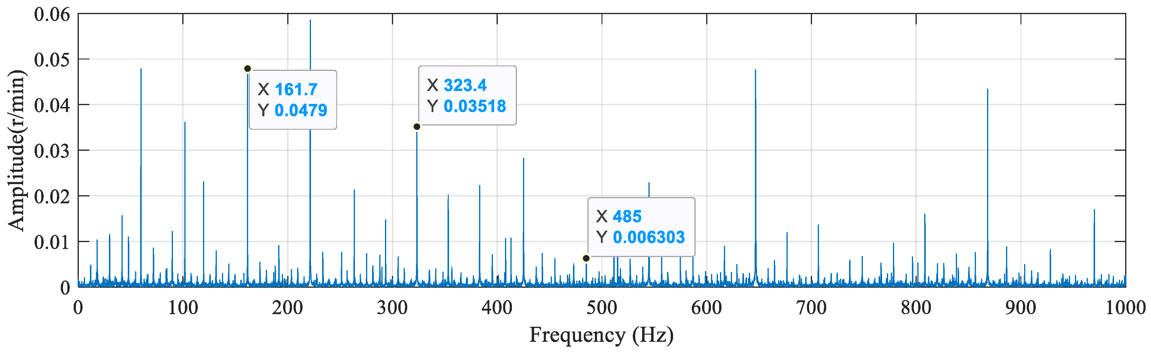
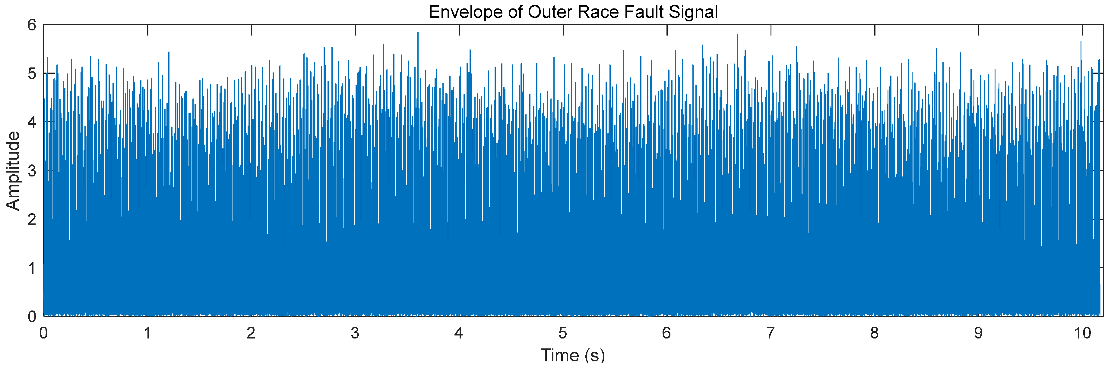
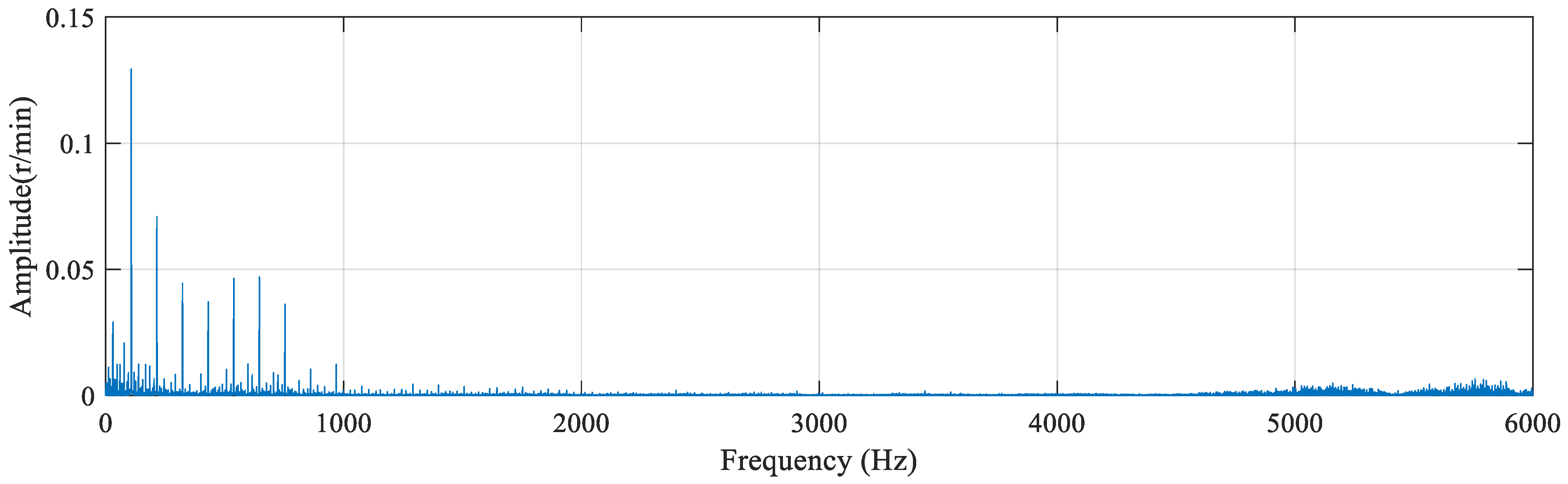
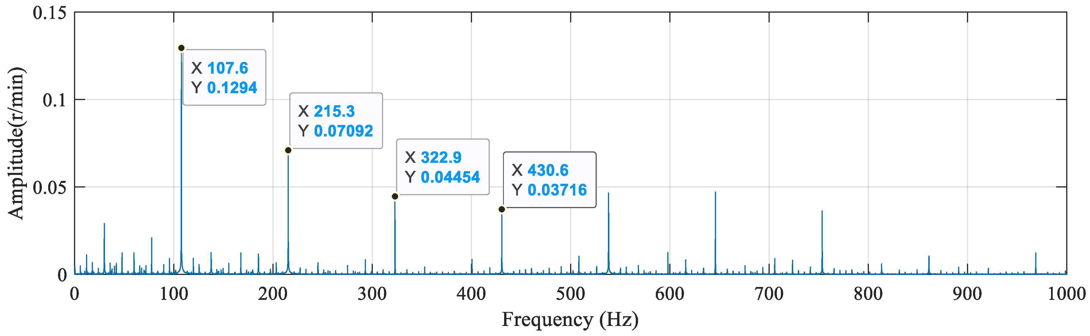
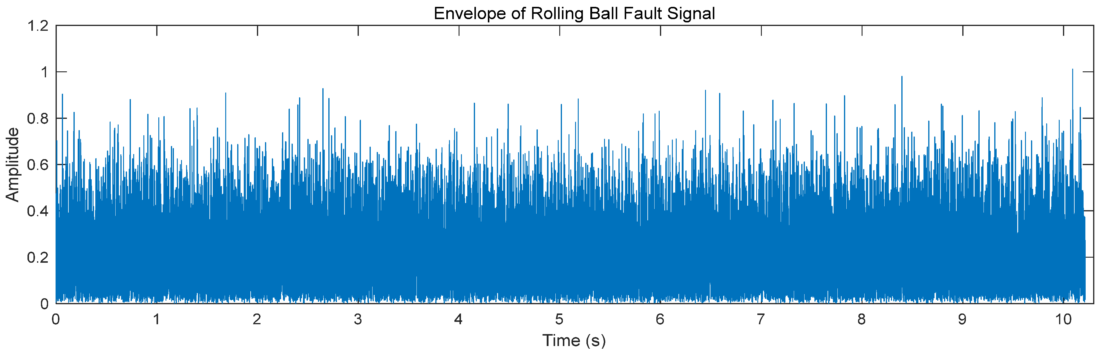
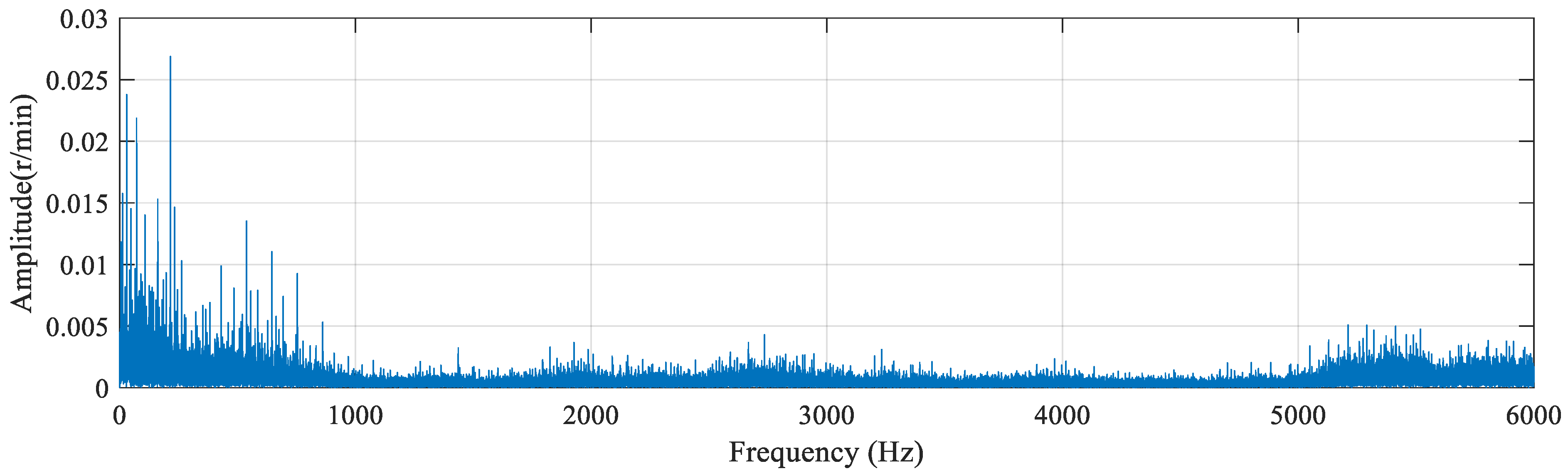
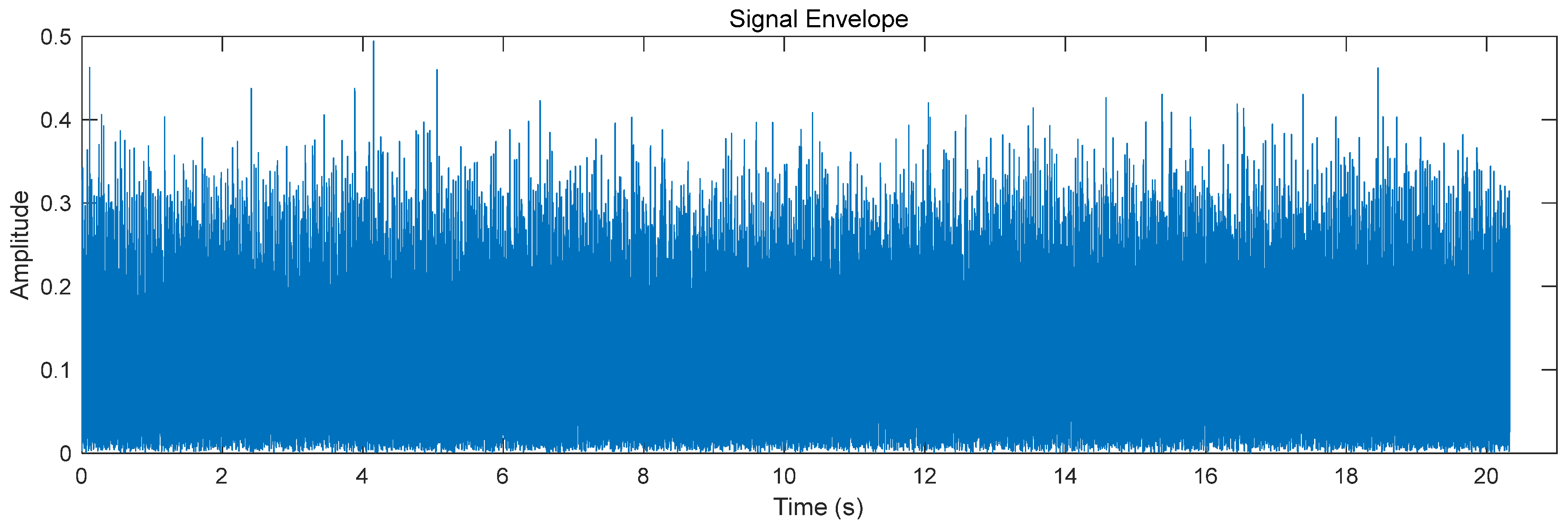
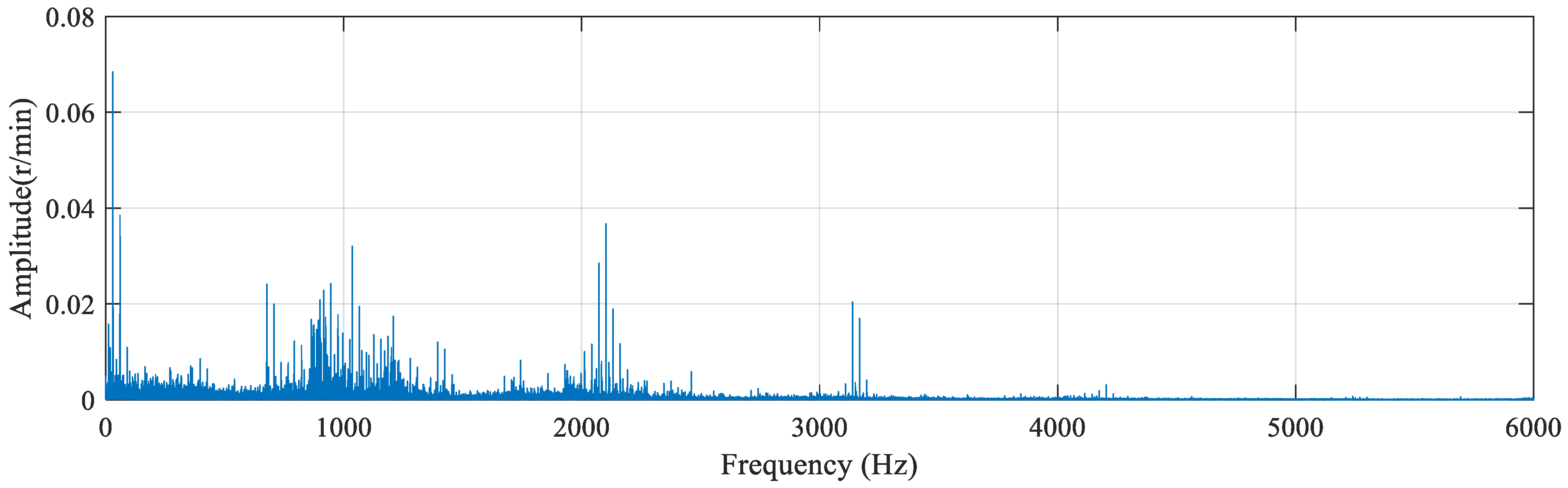
3.2. Hilbert Envelope Analysis

Hilbert transformations [14] were applied to one set of data from each of the four categories: normal signals, inner race faults, outer race faults, and rolling element faults.

A signal has both amplitude and phase information, so it can be determined as follows:

$$x\left(t\right)=A\left(t\right)\cos \left({\omega }_{0}t+\theta \left(t\right)\right)$$

(17)

By transforming the real-valued signal into a complex form, information such as the instantaneous amplitude and instantaneous frequency of the signal can be directly extracted from the real-valued signal.

$$\tilde{x}\left(t\right)=x\left(t\right)+j\tilde{x}\left(t\right)$$

(18)

$$\tilde{x}\left(t\right)=A\left(t\right)\cos \left[{\omega }_{0}t+\theta \left(t\right)\right]+jA\left(t\right)\sin \left[{\omega }_{0}t+\theta \left(t\right)\right]$$

(19)

$$\tilde{x}\left(t\right)=A\left(t\right)e^{j({\omega }_{0}t+\theta (t))}$$

(20)

$$\tilde{x}\left(t\right)=A\left(t\right)e^{j\theta (t)}{e}^{j{\omega }_{0}t}$$

(21)

where $e^{j{\omega }_{0}t}$ is the complex carrier signal and $A\left(t\right)e^{j\theta (t)}$ is the complex envelope.

$$\left|\tilde{x}\left(t\right)\right|=\left|A\left(t\right)e^{j\theta \left(t\right)}\right|=\left|A\left(t\right)\right|$$

(22)

The absolute value of the analytical signal is the envelope signal.

The amplitude–frequency plots obtained through fast Fourier transform are illustrated in Figure 5, Figure 6, Figure 7, Figure 8, Figure 9, Figure 10, Figure 11, Figure 12, Figure 13, Figure 14, Figure 15 and Figure 16.

The data within the first 1000 Hz of the envelope signal related to the inner race fault were analyzed. Based on established experience, the characteristic frequency of the inner race fault in the rolling bearing was identified as 161.7 Hz, with the second harmonic located at 323.4 Hz.

The data within the first 1000 Hz of the envelope signal related to the outer race fault were analyzed. Based on established experience, the characteristic frequency of the outer race fault in the rolling bearing was identified as 107.6 Hz, with the second harmonic located at 323.4 Hz.

The data within the first 1000 Hz of the envelope signal associated with the rolling element fault were analyzed. Based on established experience, the characteristic frequency of the rolling element fault in the rolling bearing was identified as 107.7 Hz.

The data within the first 1000 Hz of the normal signal were analyzed. Based on established experience, the rotational frequency was identified as 59.87 Hz.

From the perspective of fault identification accuracy, spectral analysis and Hilbert envelope analysis serve as common diagnostic methods that can reveal certain characteristics of faults. However, these methods heavily rely on existing experience and patterns, which limits their effectiveness. For instance, the spectra of inner race faults and rolling element faults often share many similarities, making their distinguishing features less pronounced and sometimes difficult to discern, potentially leading to diagnostic errors.

The fault signals in rolling bearings are frequently influenced by modulation components and fault interferences, particularly in complex and variable fault environments and mechanisms. This can affect the fault characteristic frequencies of the monitored bearing components, impacting the accuracy of fault diagnosis. Therefore, while the methods described in this section are considered as references, they were not adopted for fault feature extraction or identification in this study.

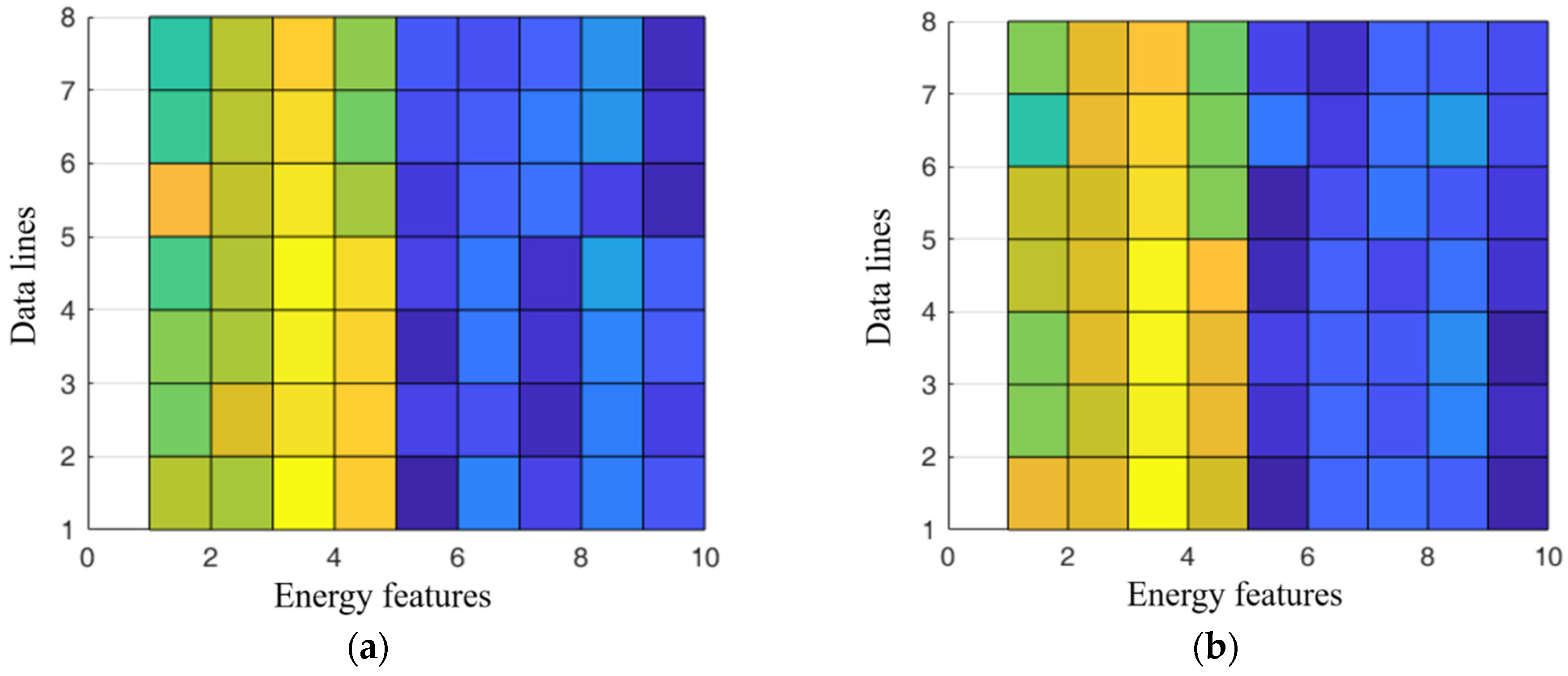
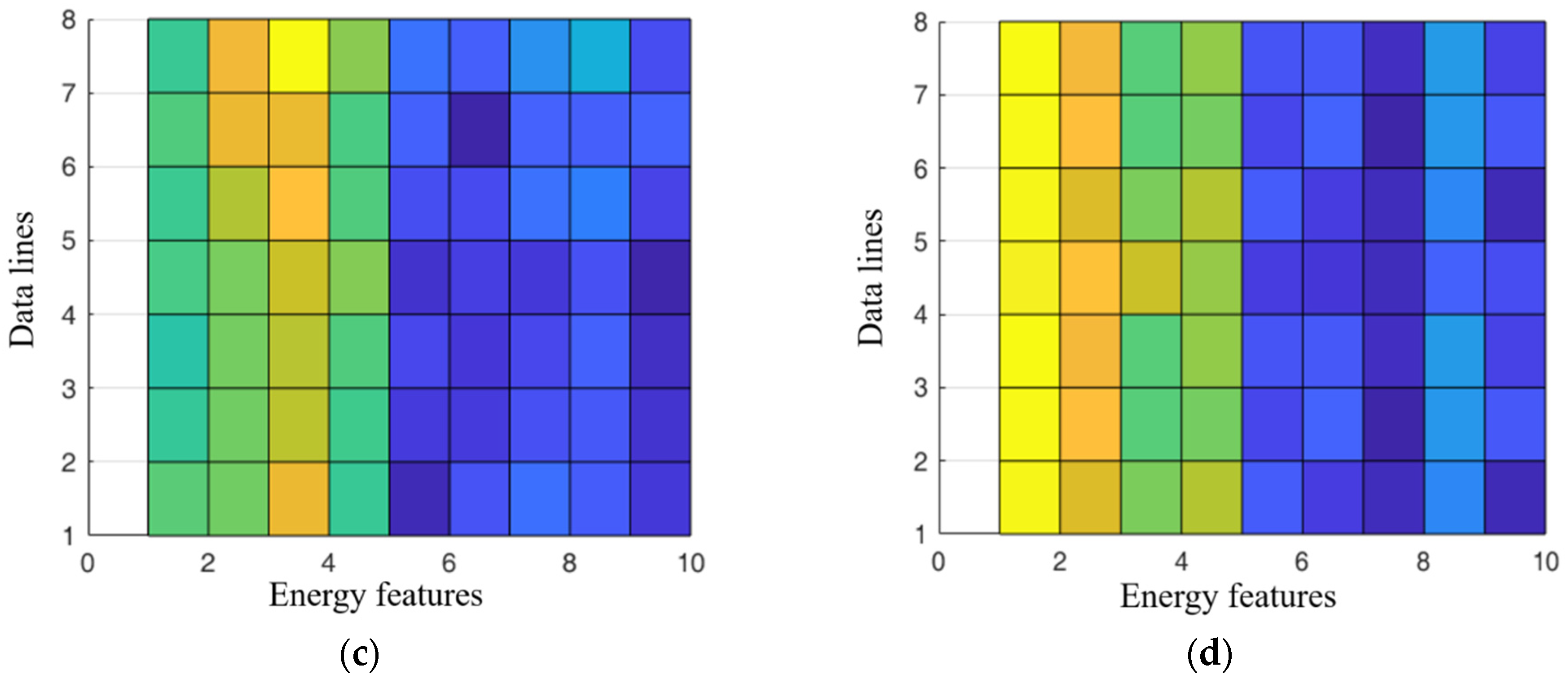
3.3. Extraction of Data Energy Features

The time-domain signals were transformed into the frequency domain using Fourier transform, and the power spectral density was calculated for various frequency ranges. By constructing a feature matrix based on the differences in energy, we completed the feature extraction work. A dataset of 400 samples was established for subsequent training and testing. Each sample contained 8 rows by 10 columns of data, where the 10 columns represented the power spectral density and its variations across different frequency bands. An example of an inner race fault sample is illustrated in

Table 2. Inner race fault sample.

PSD	PSD1	PSD2	PSD3	PSD4	Difference1	Difference2	Difference3	Difference4	Difference5	Difference6
Channel1	0.46797891	0.43254647	0.57853334	0.53355775	0.03543243	0.14598686	0.04497558	0.11055443	0.10101128	0.06557885
Channel2	0.37865839	0.44737680	0.57607983	0.52894089	0.06871841	0.12870303	0.04713894	0.19742144	0.08156409	0.15028250
Channel3	0.41025924	0.46283475	0.57174661	0.52734527	0.05257551	0.10891185	0.04440133	0.16148736	0.06451052	0.11708603
Channel4	0.43215609	0.43742075	0.60494556	0.54830006	0.00526466	0.16752481	0.05664550	0.17278947	0.11087931	0.11614397
Channel5	0.49463017	0.49092525	0.56641170	0.43228196	0.00370492	0.07548644	0.13412974	0.07178152	0.05864329	0.06234821
Channel6	0.34663556	0.43162422	0.53340069	0.38812957	0.08498866	0.10177648	0.14527113	0.18676514	0.04349465	0.04149401
Channel7	0.39908428	0.45614893	0.52513471	0.42520456	0.05706465	0.06898578	0.09993014	0.12605043	0.03094436	0.02612028
Channel8	0.33629645	0.41131140	0.54140532	0.44243298	0.07501495	0.13009392	0.09897234	0.20510887	0.03112158	0.10613653

.

The extracted features were subjected to visualization processing, as depicted in Figure 17.

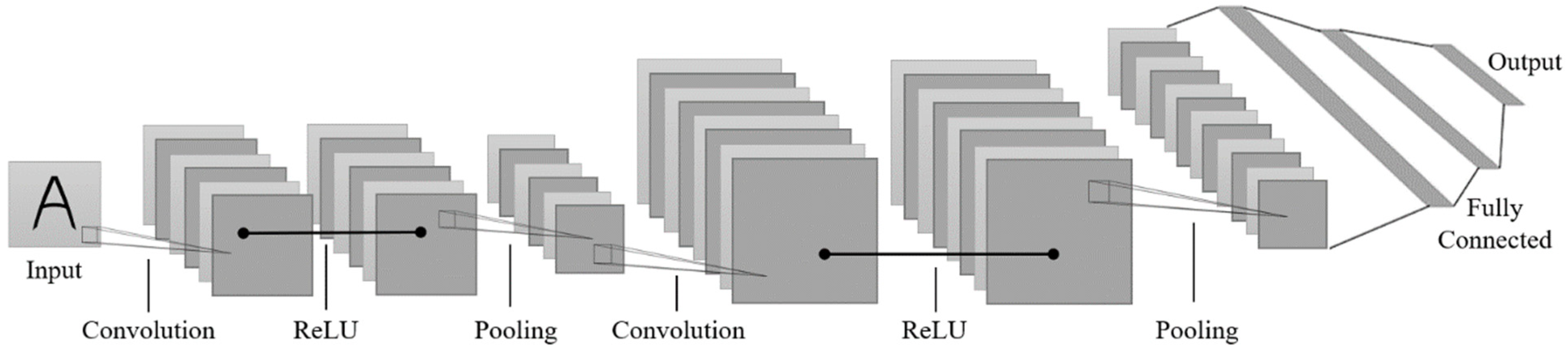
3.4. Convolutional Neural Network Architecture

A complete convolutional neural network (CNN) typically consists of four primary components: convolutional layers, pooling layers, activation layers, and fully connected layers [19]. The convolutional layers are primarily responsible for feature extraction, while the pooling layers reduce the spatial dimensions of the feature maps. The activation layers introduce non-linearity into the network, and the fully connected layers perform classification of the extracted high-dimensional features. Building a complete convolutional neural network for practical fault detection usually has the following parts: data preprocessing, building a convolutional neural network structure, defining the loss function and selecting the appropriate optimizer, training the network, reasonably evaluating it with evaluation metrics, and optimizing the network and exporting it for subsequent research. A convolutional neural network is depicted in Figure 18.

3.4.1. Convolutional Layer

The convolutional layer, as a fundamental component of a convolutional neural network, typically contains multiple filters known as convolution kernels. These kernels perform convolution operations with the input to produce the desired feature maps. When data pass through a predefined convolutional layer, the size change of the feature maps follows a specific calculation rule:

$$L_{\mathrm{out}}=1+{\displaystyle \frac{L_{\mathrm{in}}-K}{S}}$$

(23)

where Lout denotes the output size length, Lin denotes the input size length, K represents the size of the convolution kernel, and S represents the stride.

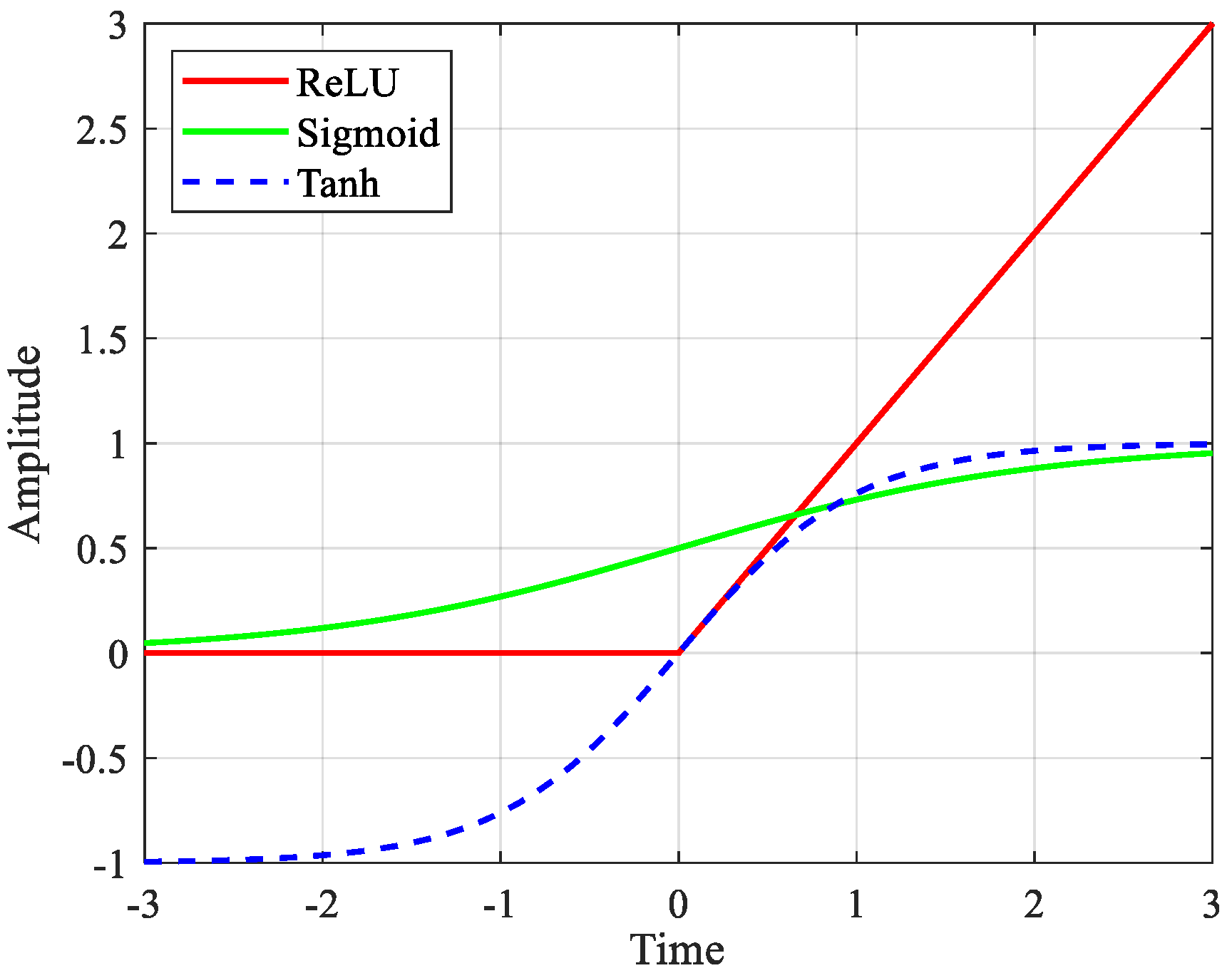
3.4.2. Activation Layer

In the structure of a convolutional neural network, to enable the entire network to capture non-linear relationships in the data, an activation layer is typically connected after the convolutional layer. The purpose of the activation layer is to perform non-linear transformations on the features. Commonly used activation functions include the sigmoid function, the rectified linear unit (ReLU) function, and the hyperbolic tangent (tanh) function [20]. These three activation functions are shown in Figure 19, and their equations are listed in

Table 3. Calculation of three types of activation functions.

Function Name	Equations
Sigmoid function	$\mathrm{Sigmod}\left(x\right)={\displaystyle \frac{1}{1+{\mathrm{e}}^{-x}}}$
Tanh function	$\mathrm{Tanh}\left(x\right)={\displaystyle \frac{{\mathrm{e}}^x-e^{-x}}{{\mathrm{e}}^x+e^{-x}}}$
ReLU function	$\mathrm{ReLU}\left(x\right)=\max \left(0,x\right)$

. The ReLU function has the characteristic of unilateral inhibition, which can help the model learn a more efficient feature representation. Due to the excellent characteristics of the ReLU function, it was used as the activation function in the construction of the convolutional neural network in this paper.

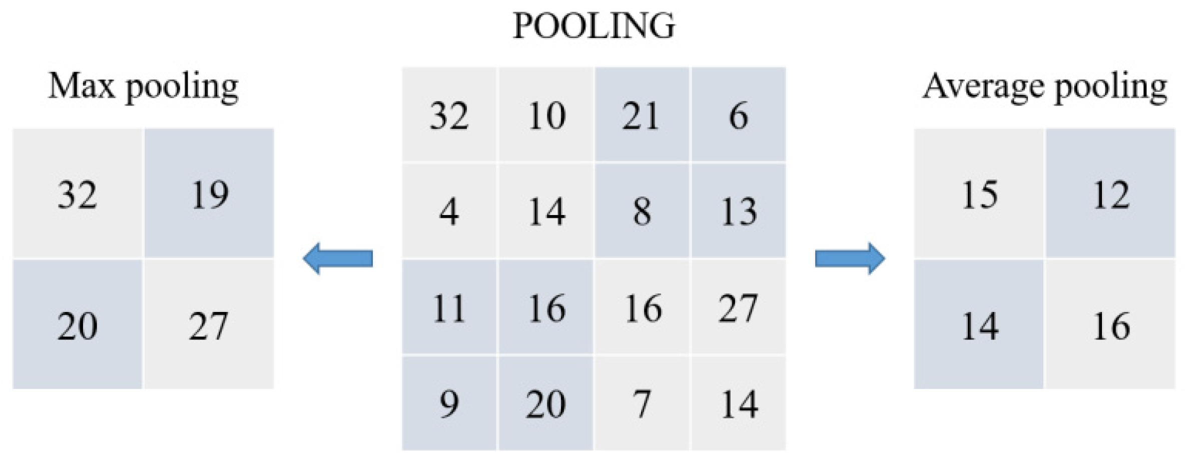
3.4.3. Pooling Layer

The pooling layer reduces the complexity of the model. By reducing the resolution of the feature map, the parameters of the neural network can be effectively reduced, and at the same time, its adaptability to input data changes in displacement and scale is enhanced. In practice, there are two common pooling methods: maximum pooling and mean pooling, as shown in Figure 20.

3.4.4. Full Connectivity Layer

A fully connected layer is one of the components of a classifier, and characterized by the fact that every neuron in the current layer is connected to all neurons in the previous layer. While operations such as convolutional, pooling, and activation layers map the original data to the hidden feature space, the fully connected layer serves to map the resulting “distributed feature representation” to the sample labeling space. The equation is as follows:

$$x_{k+1}=\Sigma W_k{x}_k+b_{k+1}$$

(24)

where $x_{k+1}$ denotes the current neuron output result; W_k denotes the connection weight; and b_k represents the size of the bias value.

3.5. Analysis of the Results of Data Energy Features

With the input to the convolutional neural network, the loss, accuracy, and confusion matrices obtained after 100 epochs of testing are shown in Figure 21 and Figure 22. In Figure 21a, the blue line represents the loss curve during training, and the orange line represents the loss curve during testing. As the iteration time increased, the loss value decreased sharply. When the epochs reached 20, the loss value reached around 1%, and the good match between the loss curves of training and testing validates the good accuracy of the proposed methods and procedures for bearing fault diagnosis. In Figure 21b, the accuracy curve during iteration is provided. The accuracy was 90% at epoch 20 and 95% at epoch 40. Around 100% accuracy was obtained at epoch 80. The significance of the proposed methods and procedures for bearing fault diagnosis are proven and can be clearly observed. The obtained results represent a good attempt at practical bearing fault diagnosis and can be implemented in actual mechanical engineering.

The confusion matrix obtained from a new test set is depicted in Figure 23. In the confusion matrices shown in Figure 22 and Figure 23, the horizontal axis represents the predicted value, and the vertical axis represents the true value. The labels 0, 1, 2, and 3 respectively represent four fault types: normal, inner race fault, outer race fault, and rolling element fault. If the obtained results are mainly distributed on the diagonal, the model can effectively classify faults. In Figure 23a, the total number of test sets was 180, of which 173 were correctly predicted, and the accuracy reached 96.111%. In Figure 23b, the total number of test sets was 120, of which 115 were correctly predicted, and the accuracy reached 95.833%. This good accuracy can be implemented in practical bearing fault diagnosis to detect different types of bearing faults for accurate fault detection.

3.6. Analysis of the Results of Data Recurrence Features

Incorporating the recurrence rate as a feature can provide the model with additional dynamic information, making it a highly effective analytical tool.

Construction of a Convolutional Neural Network Model

The structural parameters of the convolutional neural network model, based on data recurrence features, are delineated in

Table 4. Structure parameters of the convolutional neural network model based on data recurrence features.

Layer Name	Type	Input Size	Kernel Size	Stride	Padding	Output Channels	Output Size	Activation Function
input	Input	8 × 11 × 1	-	-	-	-	8 × 11 × 1	-
conv1	Convolutional	8 × 11 × 1	3 × 3	1	1	6	6 × 9 × 10	ReLU
pool1	Pooling	6 × 9 × 10	2 × 2	2	0	-	3 × 5 × 6	-
conv2	Convolutional	3 × 5 × 6	3 × 3	1	1	12	3 × 3 × 12	ReLU
pool2	Pooling	3 × 3 × 12	2 × 2	2	0	-	1 × 2 × 12	-
conv3	Convolutional	1 × 2 × 12	3 × 3	1	1	24	1 × 1 × 24	ReLU
flatten	Flatten	1 × 1 × 24	-	-	-	-	96	-
fc1	Fully Connected	96	-	-	-	4	4	Softmax

.

With the input to the convolutional neural network, the loss, accuracy, and confusion matrices obtained after 100 epochs of testing are depicted in Figure 24 and Figure 25. In Figure 24a, the blue line represents the loss curve during training, and the orange line represents the loss curve during testing. As the number of iterations increased, the loss value decreased sharply. By the time the number of epochs reached 20, the loss value stabilized at approximately 1%. The close alignment of the loss curves for the training and testing indicates the high accuracy of the proposed methods and procedures in diagnosing bearing faults. In Figure 24b, the accuracy curve over the course of iterations is illustrated. At 25 epochs, the accuracy stood at 90%, rising to 95% by 30 epochs. An accuracy nearing 100% was achieved by 60 epochs. The significance of the proposed methods and procedures for bearing fault diagnosis are proven and and can be clearly observed.

The confusion matrix obtained from a new test set is depicted in Figure 26. In the confusion matrices shown in Figure 25 and Figure 26, the horizontal axis represents the predicted value, and the vertical axis represents the true value. The labels 0, 1, 2, and 3 respectively represent four fault types: normal, inner race fault, outer race fault, and rolling element fault. If the obtained results are mainly distributed on the diagonal, the model can effectively classify the faults. As shown in Figure 26a, the total number of test sets was 180, of which 176 were correctly predicted, and the accuracy reached 97.778%. As shown in Figure 26b, the total number of test sets was 120, of which 117 were correctly predicted, and the accuracy reached 97.500 %.

4. Model Comparison

A comparison of the model accuracy rates obtained from the two methods is depicted in

Table 5. Comparison of two models.

Accuracy	Energy Model	Recurrence Rate Model
Group 1	96.667%	96.667%
Group 2	96.111%	97.778%
Group 3	95.833%	97.500%
Group 4	97.619%	99.048%
Average	96.557%	97.748%

. The average accuracy rate of the convolutional neural network model based on energy analysis was 96.557%, and the average accuracy rate of the model based on data recurrence features was 97.748%. Since the method involving added recurrence rates incorporates dynamic characteristics, the models derived from these features converged faster and exhibited stronger generalization capabilities. Compared to the model that used only energy as an input feature, the model with additional dynamic features achieved faster final convergence of the loss values and higher accuracy, yielding better overall model performance. Thus, the optimal combination of data features can be obtained, which provides better data preprocessing choices for practical bearing fault diagnosis.

A bar chart comparing the accuracy rates is shown in Figure 27.

5. Conclusions

Bearing health is important for the working life of rotating machinery. This research focused on the intelligent diagnosis of bearing faults. Through accurate and systematic data preprocessing procedures and neural networks, the intelligent diagnosis of bearing faults was successfully performed. These included a CNN grounded in data energy analysis and recurrence characteristics. The proposed data preprocessing procedures and intelligent algorithms have demonstrated their efficiency and accuracy in categorizing diverse fault types, exhibiting high precision in identification and robust generalization. The main contributions of the paper can be summarized as follows:

(1)

Recurrence quantity spectrums were defined to obtain a comprehensive dataset with enhanced features.

(2)

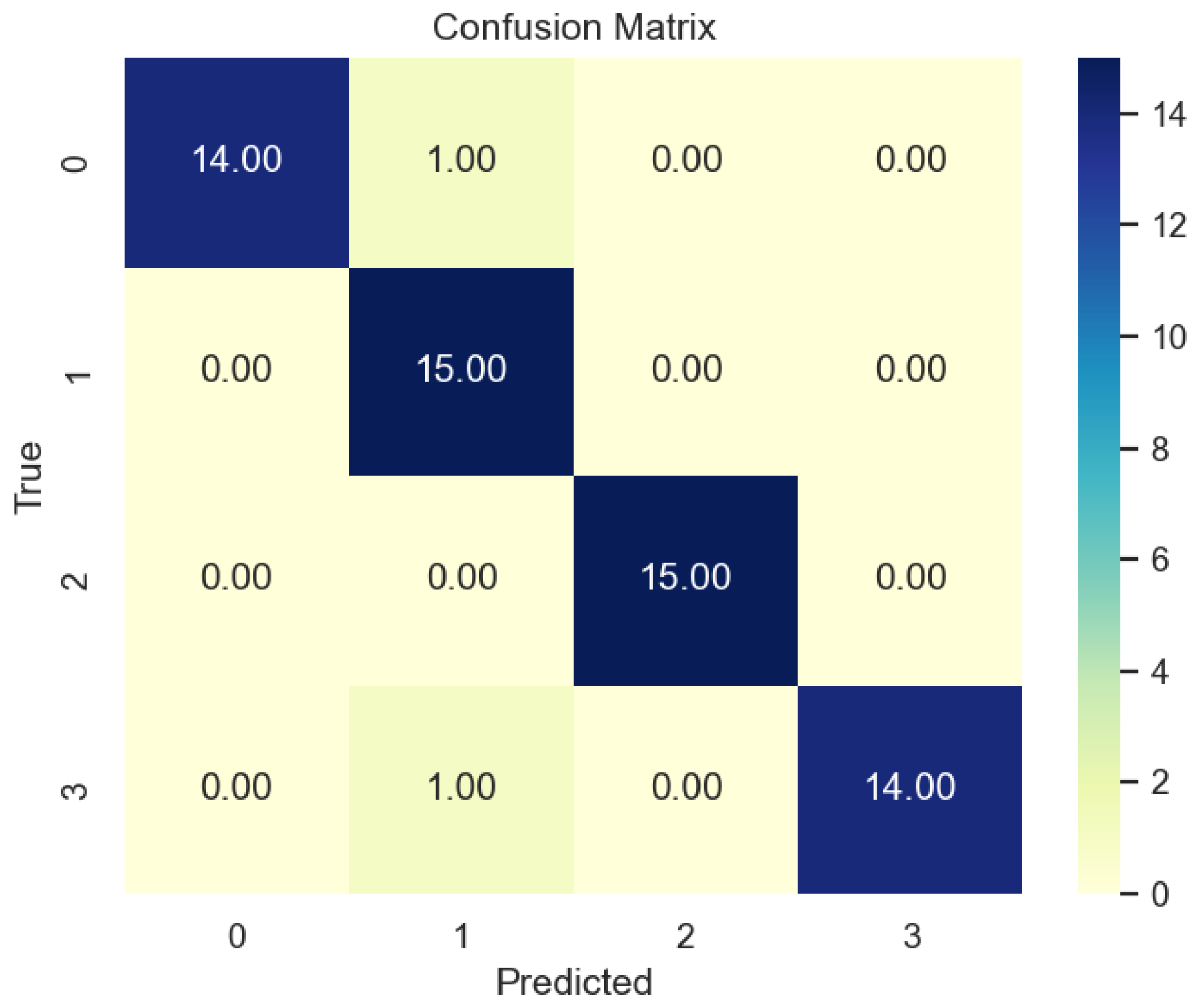
A machine learning framework based on a convolutional neural network (CNN) was constructed. The activation functions in the activation layer were optimized for better fault diagnosis. The feature matrices were specifically defined to identify the subtlest defects of bearings accurately.

(3)

Comparisons of energies, recurrence quantification, and amplitude–frequency characteristics for bearing fault detection were conducted to assess the accuracy, computational efficiency, and robustness.

(4)

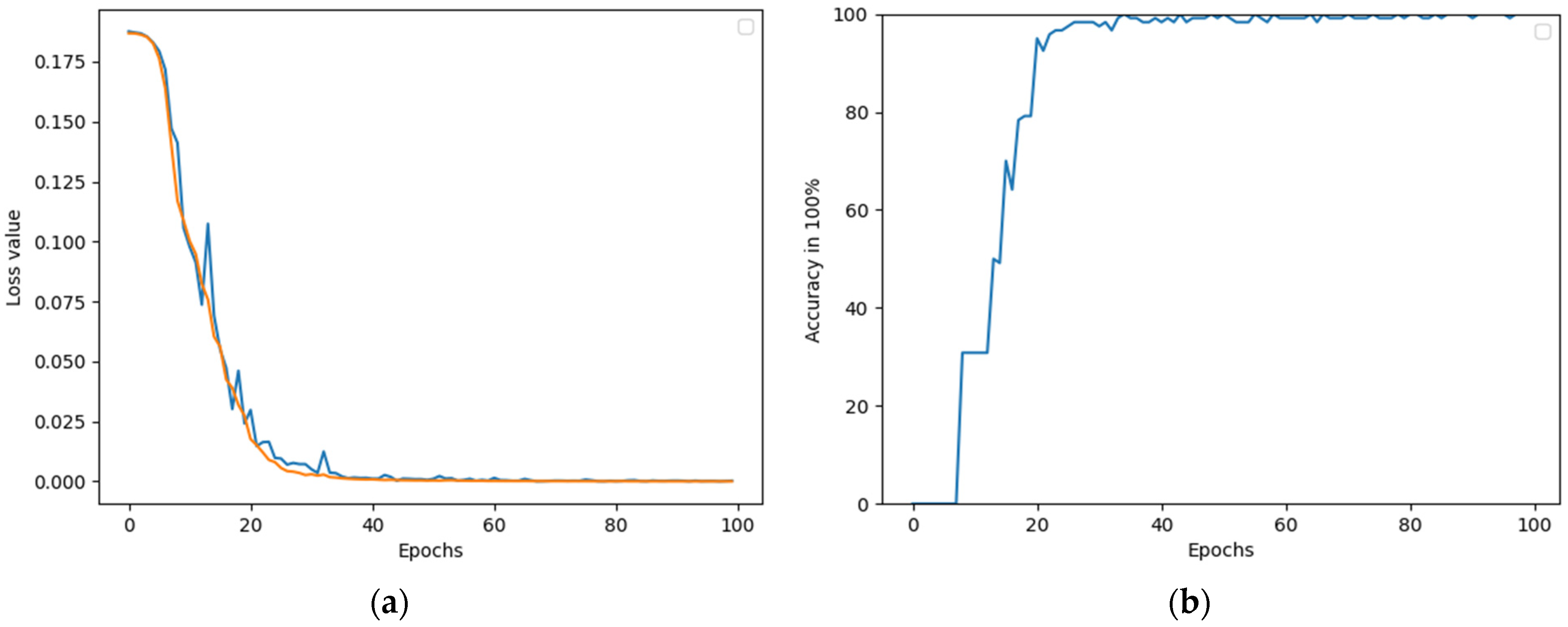
Through the delineation of training and testing sets, an accuracy over 98% was obtained, accompanied by improved generalization ability and robustness.

(5)

This research developed a more efficient fault detection procedure and algorithms, which can serve as a universal model for practical bearing fault diagnosis in engineering.

The proposed method and bearing fault diagnosis procedures are mainly based on theoretical algorithms. Future research can be planned to focus on hardware design and implementation for more practical application of the methods.

References

1. Yang, C. Research on Intelligent Diagnosis Methods of Mechanical Faults Based on Uncertainty Theory; University of Science and Technology of China: Hefei, China, 2009; pp. 65–75, (In Chinese with English Abstract). [Google Scholar]
2. Bruna, J.; Zaremba, W.; Szlam, A.; LeCun, Y. Spectral Networks and Locally Connected Networks on Graphs. arXiv 2013, arXiv:1312.6203. [Google Scholar] [CrossRef]
3. Guo, X.; Chen, L.; Shen, C. Hierarchical adaptive deep convolution neural network and its application to bearing fault diagnosis. Measurement 2016, 93, 490–502. [Google Scholar] [CrossRef]
4. Zhang, W. Research on Bearing Fault Diagnosis Algorithm Based on Convolutional Neural Network; Harbin Institute of Technology: Harbin, China, 2017; pp. 30–55, (In Chinese with English Abstract). [Google Scholar]
5. Li, S.; Liu, G.; Tang, X.; Lu, J.; Hu, J. An Ensemble Deep Convolutional Neural Network Model with Improved D-S Evidence Fusion for Bearing Fault Diagnosis. Sensors 2017, 17, 1729. [Google Scholar] [CrossRef] [PubMed]
6. Yuan, J.H.; Han, T.; Tang, J.; An, L.Z. Intelligent fault diagnosis method for rolling bearings based on wavelet time-frequency map and CNN. J. Mach. Des. Res. 2017, 33, 93–97, (In Chinese with English Abstract). [Google Scholar]
7. Qu, J.; Yu, L.; Yuan, T.; Tian, Y.; Gao, F. Adaptive fault diagnosis algorithm for rolling bearings based on one-dimensional convolutional neural network. Chin. J. Sci. Instrum. 2018, 39, 134–143, (In Chinese with English Abstract). [Google Scholar]
8. Xiao, X.; Wang, J.; Zhang, Y.; Guo, Q.; Zong, S. An optimized two-dimensional convolutional neural network method for bearing fault diagnosis. Proc. CSEE 2019, 39, 4558–4568, (In Chinese with English Abstract). [Google Scholar]
9. Shao, S.; McAleer, S.; Yan, R.; Baldi, P. Highly accurate machine fault diagnosis using deep transfer learning. IEEE Trans. Ind. Inform. 2019, 15, 2446–2455. [Google Scholar] [CrossRef]
10. Zhao, Z.; Jiao, Y. A fault diagnosis method for rotating machinery based on CNN with mixed information. IEEE Trans. Ind. Inform. 2023, 19, 9091–9101. [Google Scholar] [CrossRef]
11. Zhao, Z.; Jiao, Y.; Zhang, X. A fault diagnosis method of rotor system based on parallel convolutional neural network architecture with attention mechanism. J. Signal Process. Syst. 2023, 95, 965–977. [Google Scholar] [CrossRef]
12. Firouzi, N.; Dohnal, F. Dynamic stability of the Mindlin-Reissner plate using a time-modulated axial force. Mech. Based Des. Struct. Mach. 2024, 1–18. [Google Scholar] [CrossRef]
13. Li, M.; Ma, W.; Liu, X. Investigation of Rolling Bearing Fault Diagnosis Based on Multi-Fractal and General Fractal Dimension. In Proceedings of the 2009 Second International Conference on Intelligent Computation Technology and Automation, Changsha, China, 10–11 October 2009; IEEE: Piscataway, NJ, USA, 2009. [Google Scholar]
14. Andrade, M.A.; Messina, A.R.; Rivera, C.A.; Olguin, D. Identification of Instantaneous Attributes of Torsional Shaft Signals Using the Hilbert Transform. IEEE Trans. Power Syst. 2004, 19, 1422–1429. [Google Scholar] [CrossRef]
15. Freeman, W.J.; Zhai, J. Simulated power spectral density (PSD) of background electrocorticogram (ECoG). Cogn. Neurodynamics 2009, 3, 97–103. [Google Scholar] [CrossRef] [PubMed]
16. Peluso, E.; Craciunescu, T.; Murari, A. A Refinement of Recurrence Analysis to Determine the Time Delay of Causality in Presence of External Perturbations. Entropy 2020, 22, 865. [Google Scholar] [CrossRef] [PubMed]
17. Yu, W.; Xu, Y.; Wang, T. Intelligent classification of the abnormal features through time-delayed reconstruction of phase states. J. Appl. Nonlinear Dyn. 2024, 6–10. [Google Scholar]
18. Available online: https://engineering.case.edu/bearingdatacenter/download-data-file (accessed on 25 August 2024).
19. Zhu, Z. Research on Domain Adaptive Algorithms for Mechanical Fault Diagnosis Based on Convolutional Neural Networks; Harbin Institute of Technology: Harbin, China, 2020; pp. 10–20, (In Chinese with English Abstract). [Google Scholar]
20. Zhang, H.; Zhang, Q.; Yu, J. Review of the development of activation functions and analysis of their properties. J. Xihua Univ. 2021, 40, 1–10. [Google Scholar]
Figure 1. Comparison between the filtered signals and the original signals (the blue line is the original signal, and the red line is the filtered signal). (a) Filter contrast 1; (b) filter contrast 2.
Applsci 14 09643 g001
Figure 2. Sinusoidal signals and their recurrence plots. (a) Sinusoidal signal; (b) recurrence plot of sinusoid signals.
Applsci 14 09643 g002
Figure 3. Lorentz signals and their recurrence plots. (a) Lorentz signal; (b) recurrence plot of Lorentz signals.
Applsci 14 09643 g003
Figure 4. Bearing failure experiment at CWRU [18].
Applsci 14 09643 g004
Figure 5. Diagram of inner race fault signal envelope.
Applsci 14 09643 g005
Figure 6. Amplitude-frequency diagram of inner race fault signal envelope.
Applsci 14 09643 g006
Figure 7. Amplitude–frequency diagram of inner race fault signal envelope (first 1000 Hz).
Applsci 14 09643 g007
Figure 8. Diagram of outer race fault signal envelope.
Applsci 14 09643 g008
Figure 9. Amplitude–frequency diagram of outer race fault signal envelope.
Applsci 14 09643 g009
Figure 10. Amplitude–frequency diagram of outer race fault signal envelope (first 1000 Hz).
Applsci 14 09643 g010
Figure 11. Diagram of rolling element fault signal envelope.
Applsci 14 09643 g011
Figure 12. Amplitude–frequency diagram of rolling element fault signal envelope.
Applsci 14 09643 g012
Figure 13. Amplitude–frequency diagram of rolling element fault signal envelope (first 1000 Hz).
Applsci 14 09643 g013
Figure 14. Diagram of normal signal envelope.
Applsci 14 09643 g014
Figure 15. Amplitude–frequency diagram of normal signal envelope.
Applsci 14 09643 g015
Figure 16. Amplitude–frequency diagram of normal signal envelope (first 1000 Hz).
Applsci 14 09643 g016
Figure 17. Visualization of data energy characteristics. (a) Inner race fault characteristics; (b) outer race fault characteristics; (c) fault characteristics of rolling elements; (d) normal features (different colors refer to different values as shown in Table 2).
Applsci 14 09643 g017aApplsci 14 09643 g017b
Figure 18. Example of a convolutional neural network structure.
Applsci 14 09643 g018
Figure 19. Three types of activation functions.
Applsci 14 09643 g019
Figure 20. Example of pooling operation.
Applsci 14 09643 g020
Figure 21. Curves of loss and accuracy. (a) Curves of loss; (b) curve of accuracy.
Applsci 14 09643 g021
Figure 22. Confusion matrix of Data Energy Features.
Applsci 14 09643 g022
Figure 23. Confusion matrices of Data Energy Features generated for the new test set. (a) New confusion matrix 1; (b) new confusion matrix 2.
Applsci 14 09643 g023
Figure 24. Curves of loss and accuracy. (a) Curves of loss, (b) Curve of accuracy.
Applsci 14 09643 g024
Figure 25. Confusion matrix of Recurrence Features.
Applsci 14 09643 g025
Figure 26. Confusion matrices generated for the new test set. (a) New confusion matrix 1; (b) new confusion matrix 2.
Applsci 14 09643 g026
Figure 27. Comparison of accuracy rates for two models.
Applsci 14 09643 g027