
Application of Different Image Processing Methods for Measuring Rock Fracture Structures under Various Confining Stresses


Abstract
:1. Introduction
2. Materials and Methods
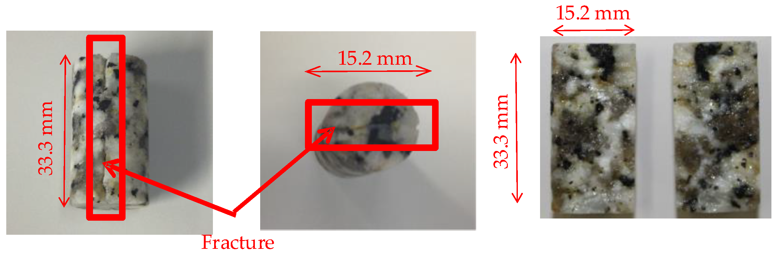
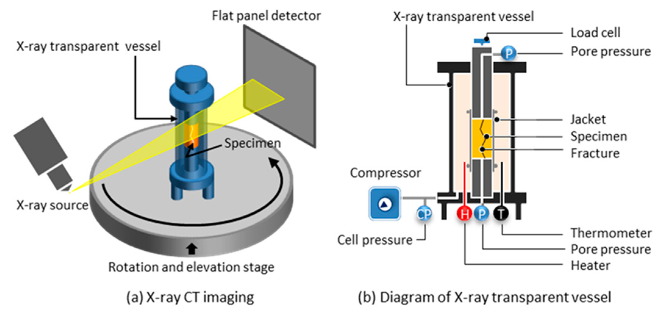
2.1. Experimental Material
2.2. Image Processing Method
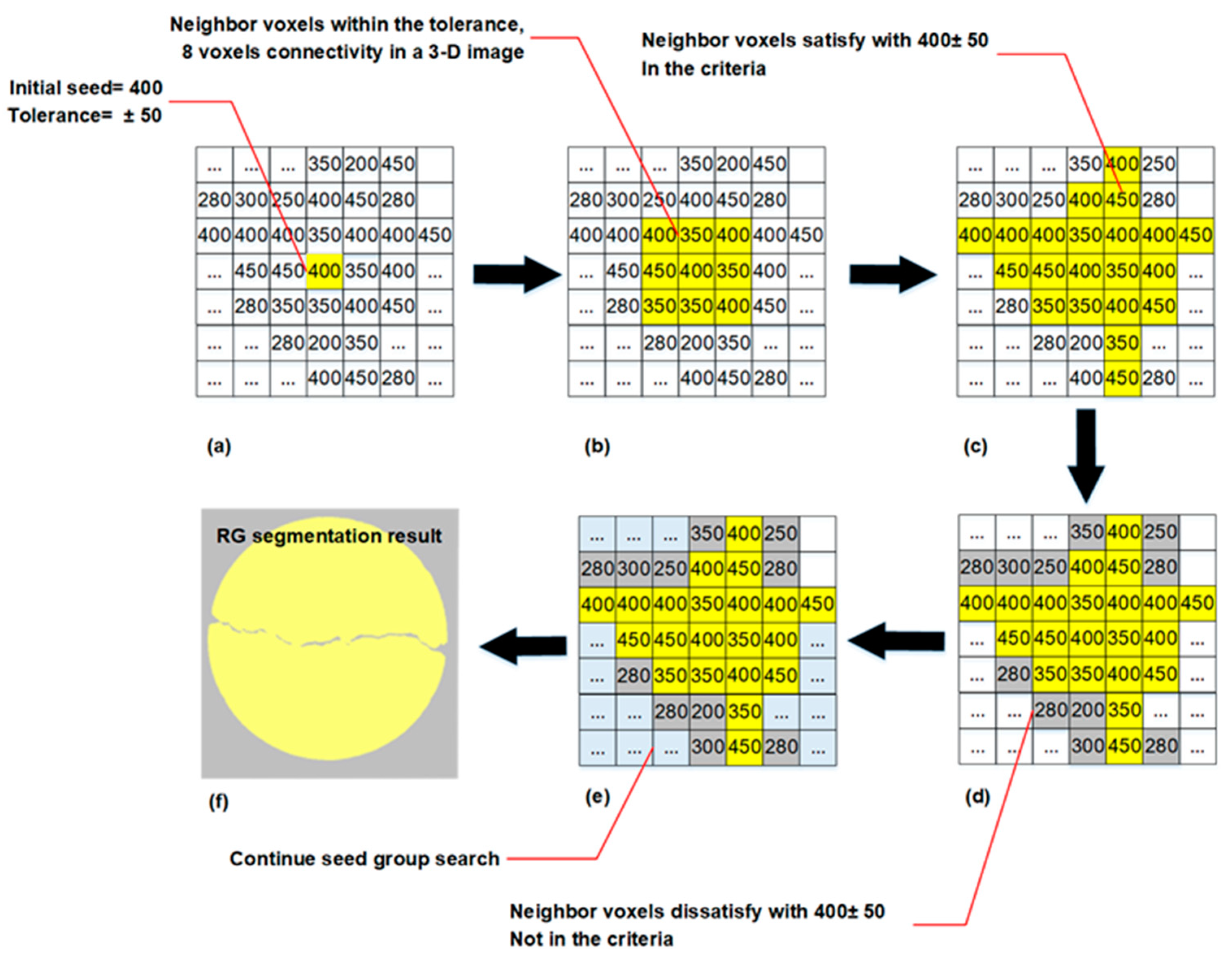
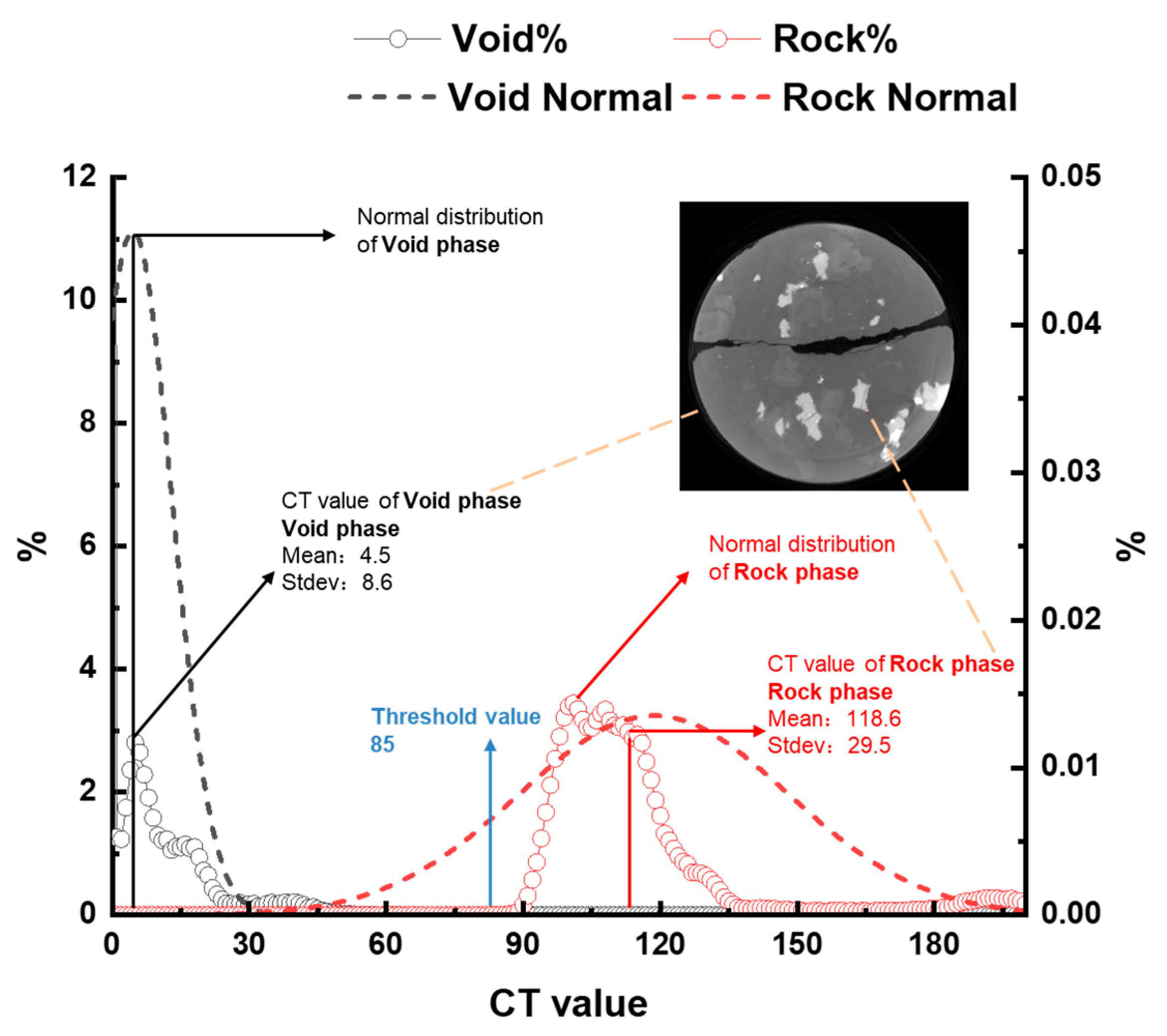
2.2.1. Region Growing Method (RG)
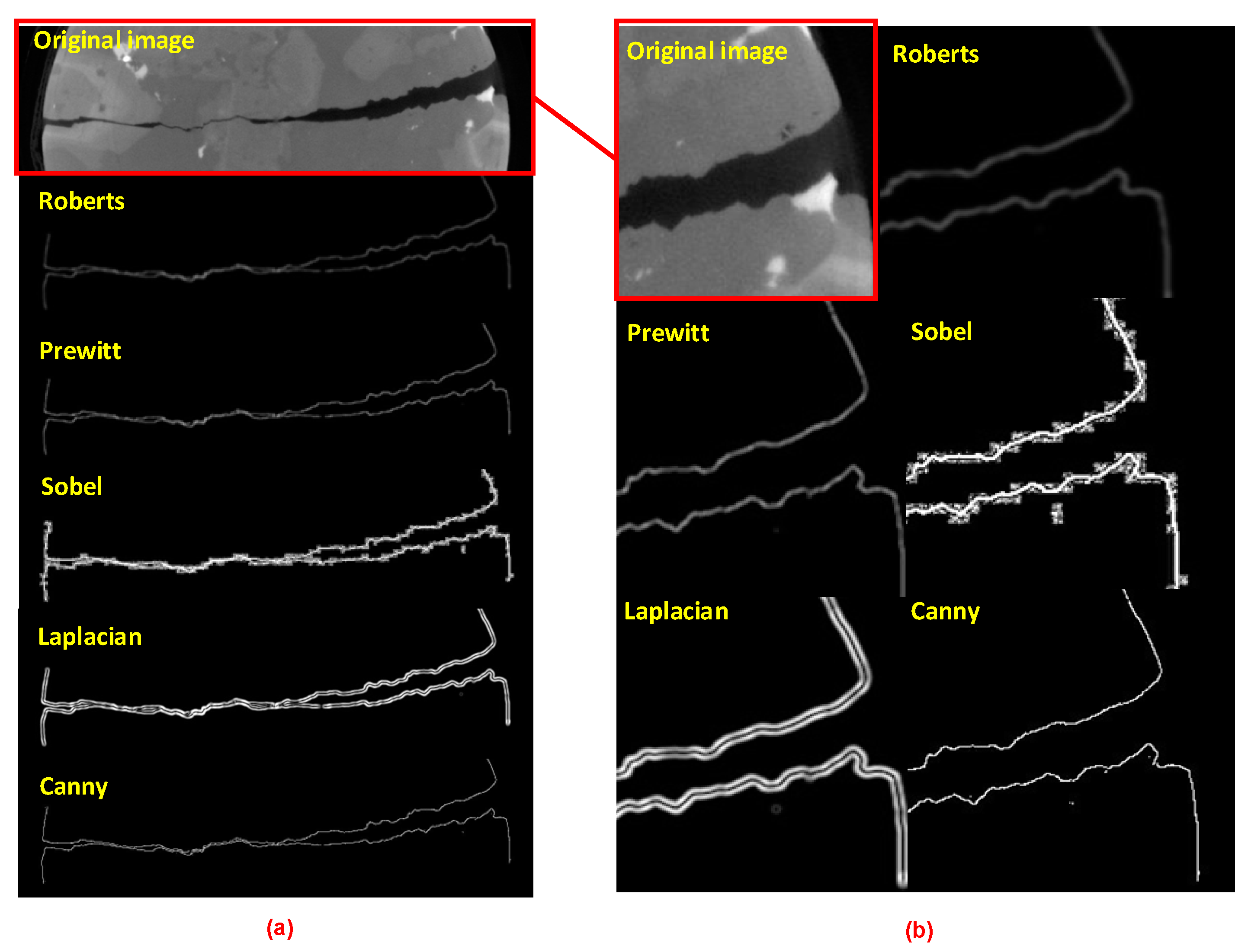
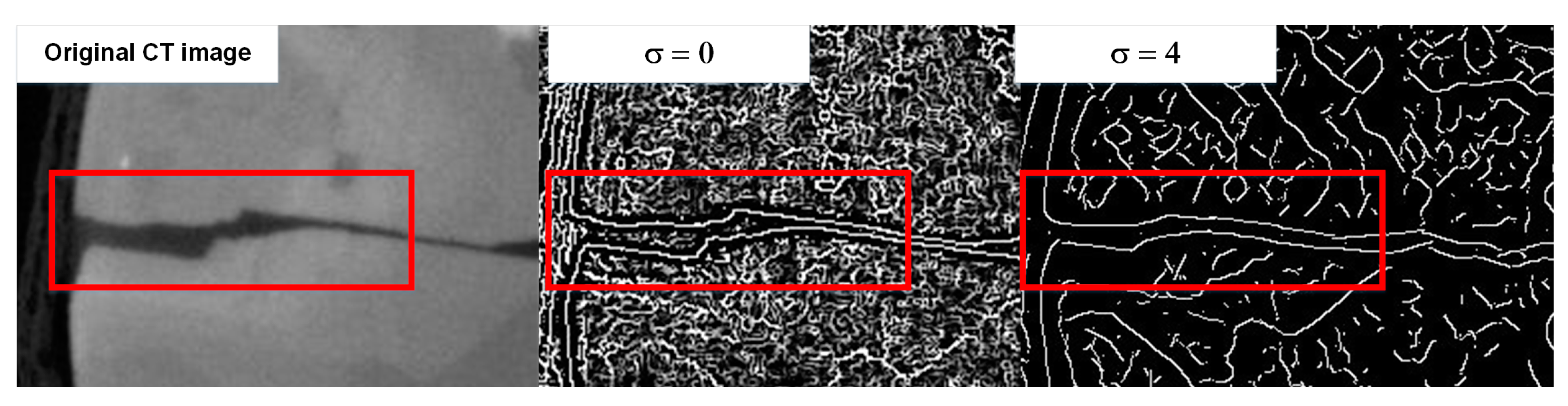
2.2.2. Edge Detection Method (ED)
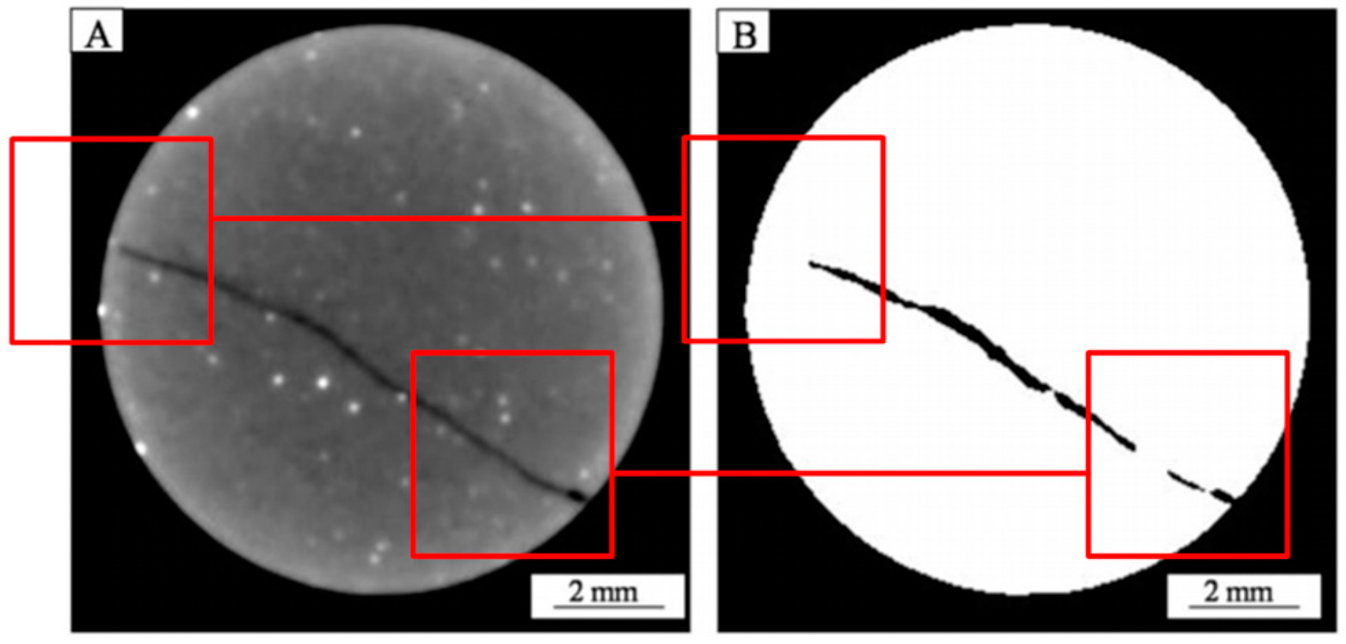
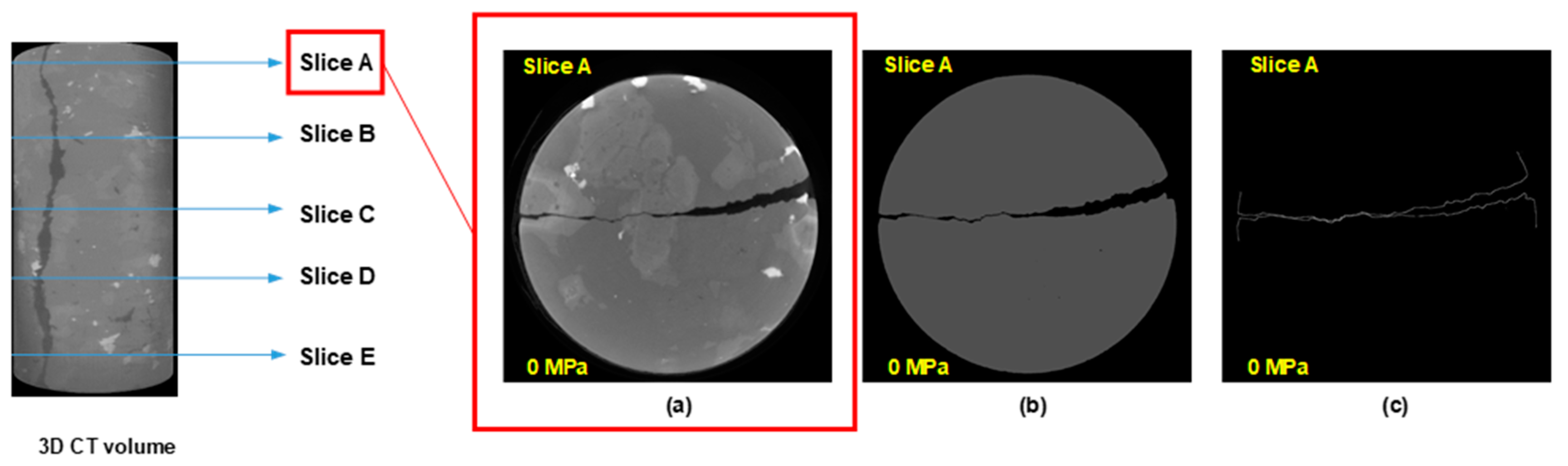
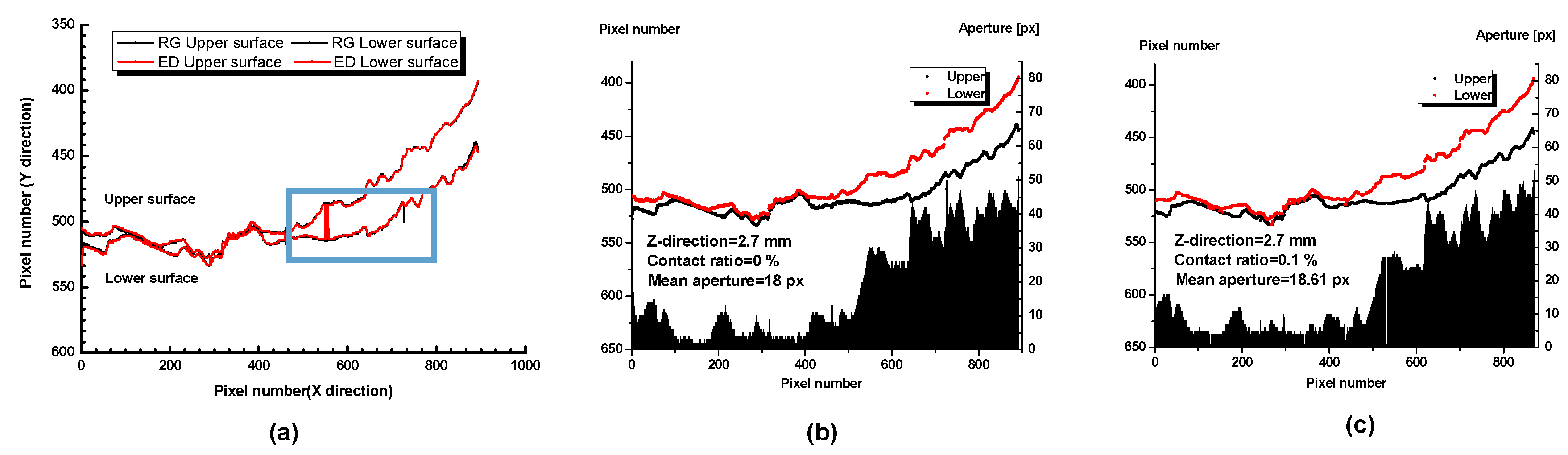
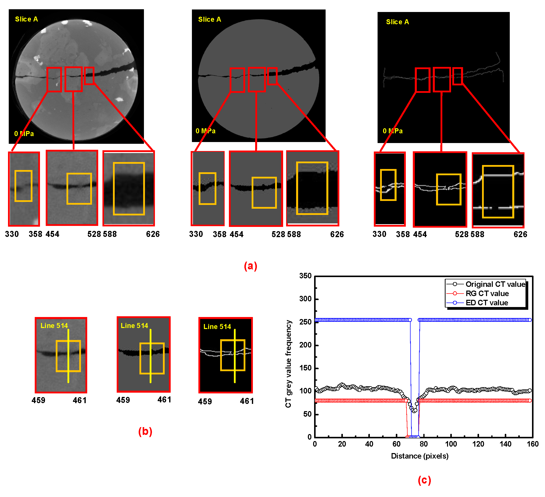
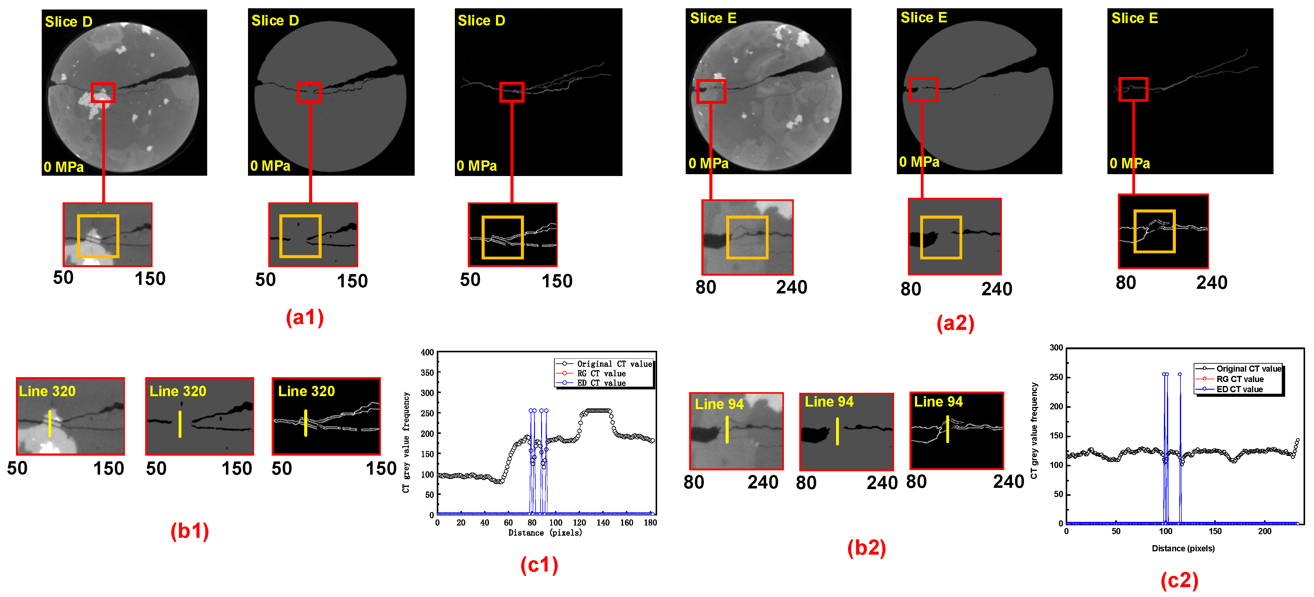
2.2.3. A Representative Image Processing Comparative Result under Region Growing and Edge Detection Method
3. Results
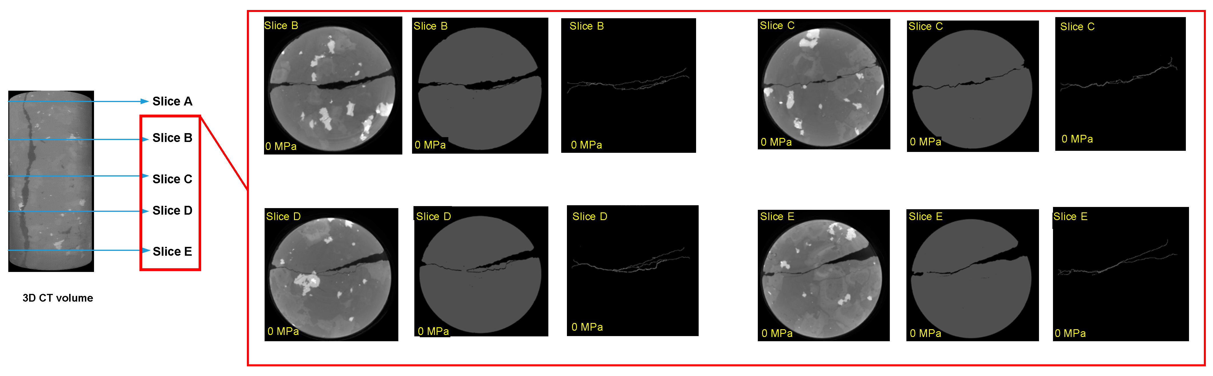
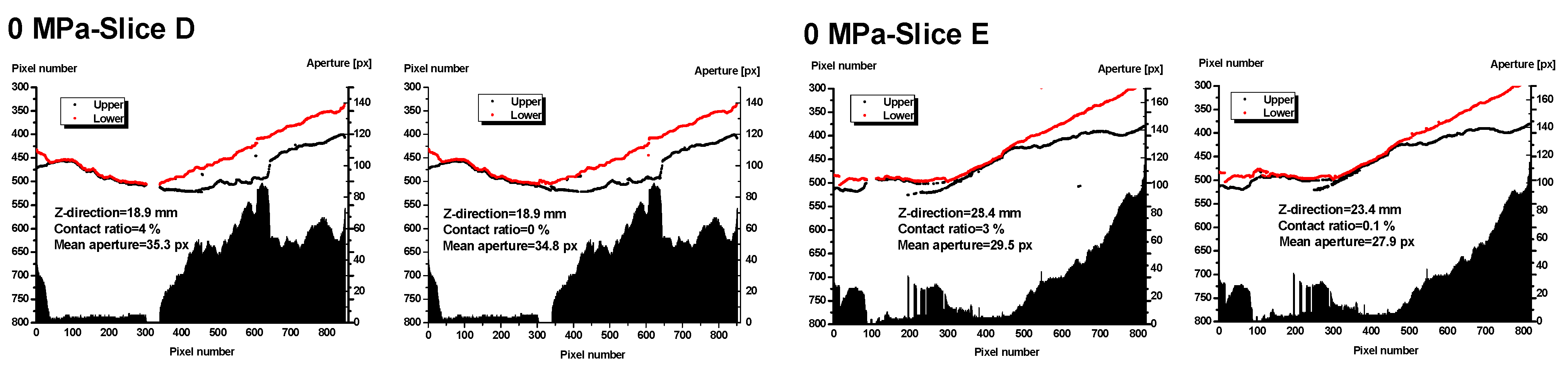
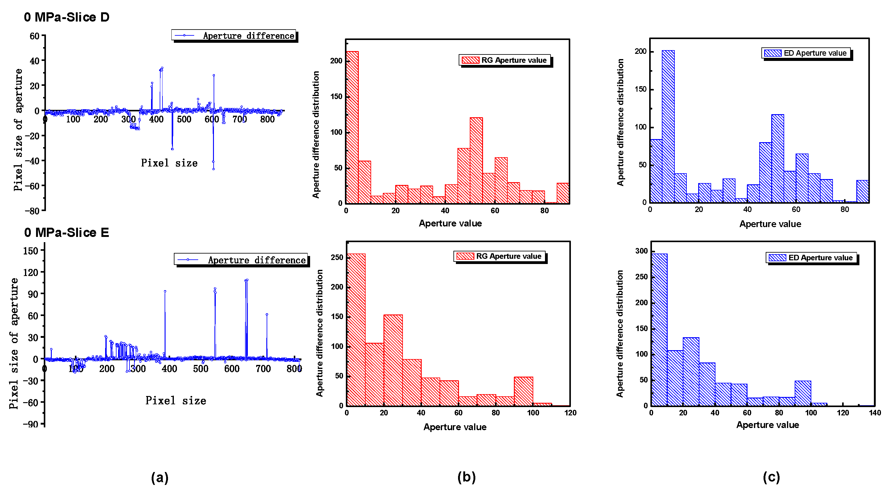
3.1. Image Processing of CT Images without Confining Stress
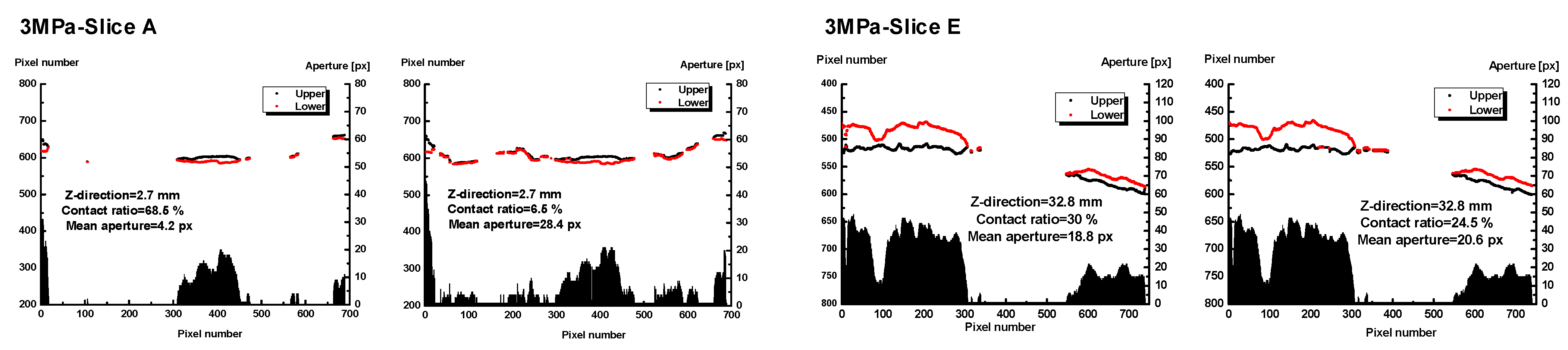
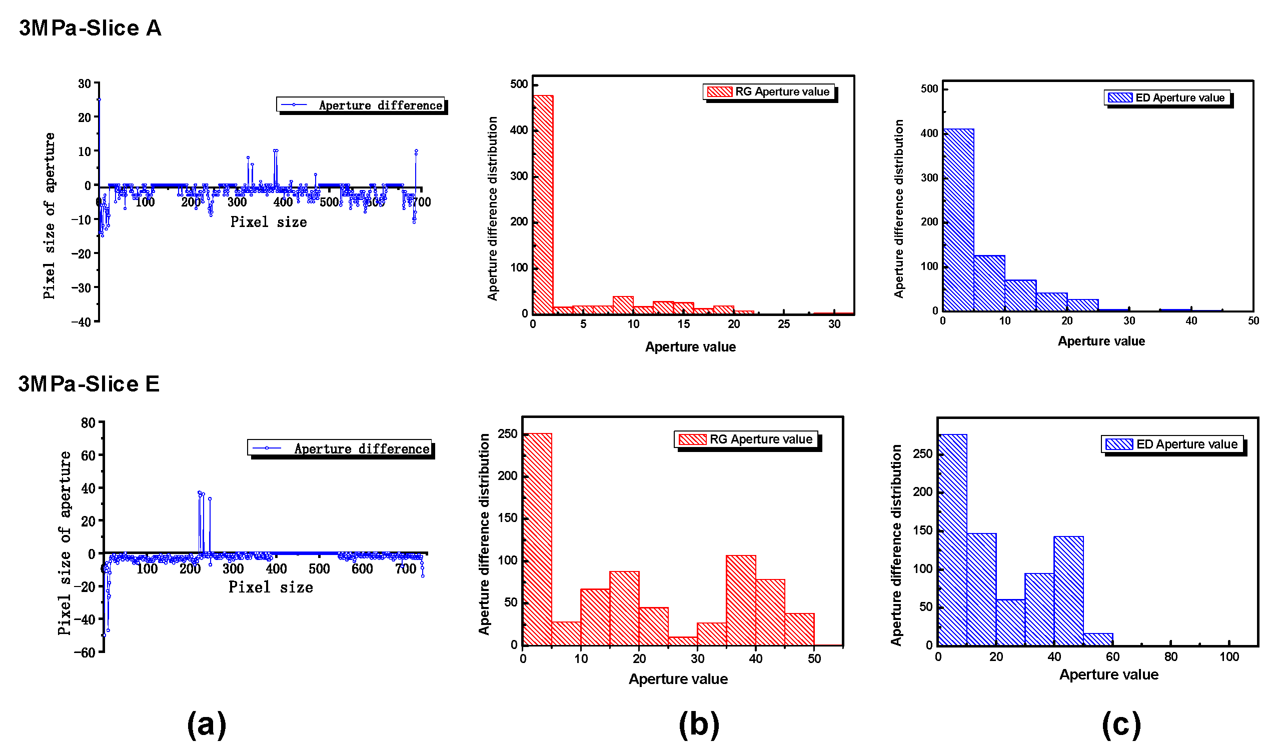
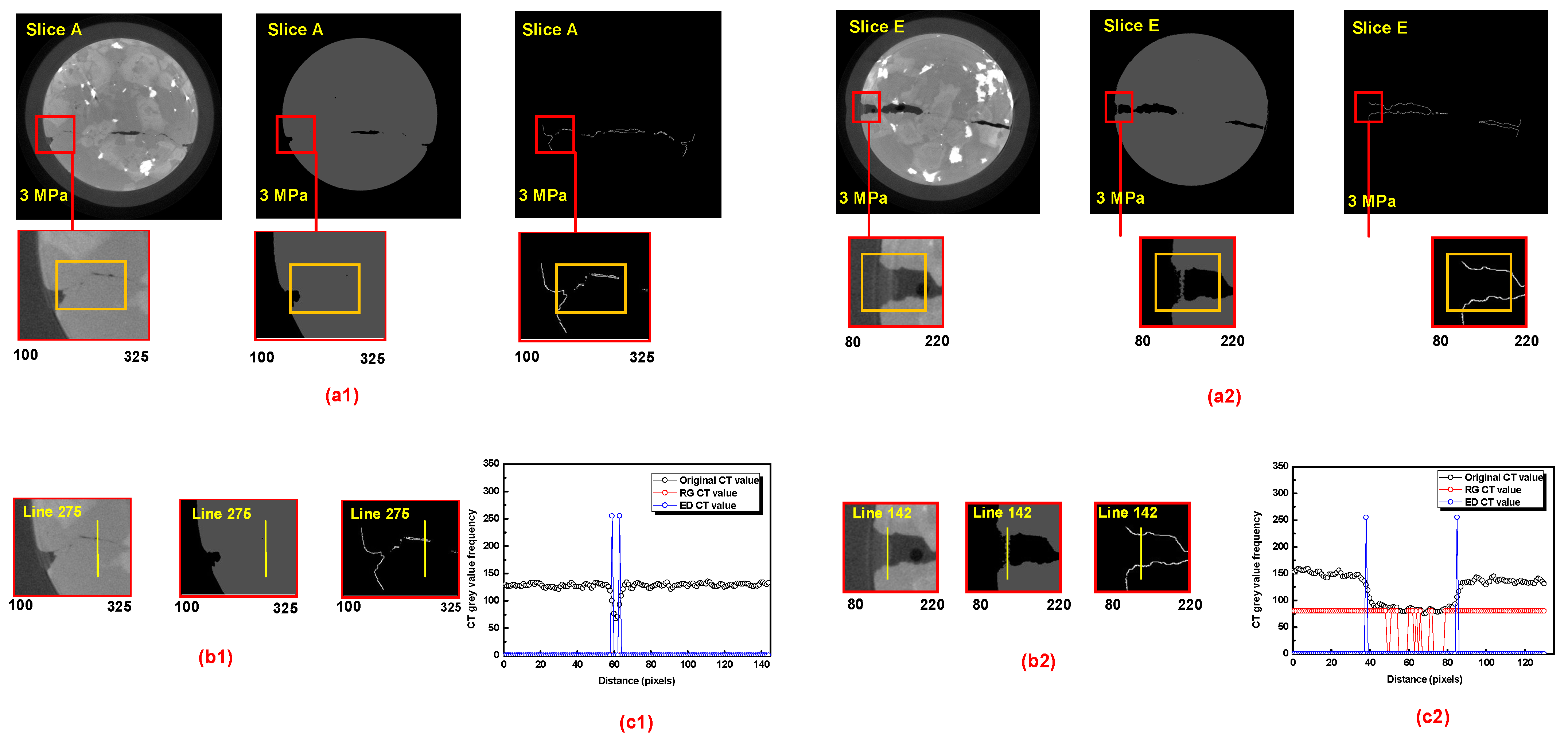
3.2. Image Processing of CT Images under Confining Stress
3.3. Summary
4. Conclusions
Author Contributions
Funding
Institutional Review Board Statement
Informed Consent Statement
Data Availability Statement
Conflicts of Interest
References
- Tsang, C.F.; Bernier, F.; Davies, C. Geo-hydromechanical processes in the excavation damaged zone in crystalline rock, rock salt, and indurated and plastic clays—In the context of radioactive waste disposal. Int. J. Rock Mech. Min. Sci. 2005, 42, 109–125. [Google Scholar] [CrossRef]
- Ellis, B.R.; Fitts, J.P.; Bromhal, G.S.; McIntyre, D.L.; Rappero, R.; Peters, C.A. Dissolution-driven permeability reduction of fractured carbonate caprock. Environ. Eng. Sci. 2013, 30, 187–193. [Google Scholar] [CrossRef] [PubMed]
- Lei, Z.H.; Zhang, Y.L.; Lin, X.J.; Shi, Y.; Zhang, Y.H.; Zhou, L.; Shen, Y.P. A thermo-hydro-mechanical simulation on the impact of fracture net-work connectivity on the production performance of a multi-fracture enhanced geothermal system. Geothermics 2024, 122, 103070. [Google Scholar] [CrossRef]
- McGuire, T.P.; Elsworth, D.; Karcz, Z. Experimental measurements of stress and chemical controls on the evolution of fracture permeability. Transp. Porous Med. 2013, 98, 15–34. [Google Scholar] [CrossRef]
- Xie, Y.C.; Liao, J.X.; Zhao, P.F.; Xia, K.W.; Li, C.B. Effects of fracture evolution and non-Darcy flow on the thermal performance of enhanced geothermal system in 3D complex fractured rock. Int. J. Min. Sci. Technol. 2024, 34, 443–459. [Google Scholar] [CrossRef]
- Silveira, C.S.d.; Alvim, A.C.M.; Oliva, J.d.J.R. Radionuclide Transport in Fractured Rock: Numerical Assessment for High Level Waste Repository. Sci. Technol. Nucl. Install. 2013, 2013, 827961. [Google Scholar] [CrossRef]
- Elsworth, D.; Yasuhara, H. Short-Timescale Chemo-Mechanical Effects and their Influence on the Transport Properties of Fractured Rock. Pure Appl. Geophys. 2006, 163, 2051–2070. [Google Scholar]
- Danko, G.; Bahrami, D. A new T-H-M-C model development for discrete-fracture EGS studies. GRC Trans. 2012, 36, 383–392. [Google Scholar]
- Ghassemi, A. A review of some rock mechanics issues in geothermal reservoir development. Geotech. Geol. Eng. 2012, 30, 647–664. [Google Scholar] [CrossRef]
- Abdullah, S.; Wang, K.; Chen, X.H.; Khan, M. The impact of thermal transport on reactive THMC model for carbon capture and storage. Geomech. Energy Environ. 2023, 36, 100511. [Google Scholar] [CrossRef]
- Xu, H.R.; Liu, G.H.; Zhao, Z.H.; Ma, F.; Wang, G.L.; Chen, Y.D. Coupled THMC modeling on chemical stimulation in fractured geothermal reservoirs. Geothermics 2024, 116, 102854. [Google Scholar] [CrossRef]
- Polak, A.; Elsworth, D.; Yasuhara, H.; Grader, A.; Halleck, P. Permeability reduction of a natural fracture under net dissolution by hydrothermal fluids. Geophys. Res. Lett. 2003, 30. [Google Scholar] [CrossRef]
- Yasuhara, H.; Polak, A.; Mitani, Y.; Grader, A.S.; Halleck, P.M.H.; Elsworth, D. Evolution of fracture permeability through fluid–rock reaction under hydrothermal conditions. Earth Planet. Sci. Lett. 2006, 244, 186–200. [Google Scholar] [CrossRef]
- Yasuhara, H.; Elsworth, D. Compaction of a Rock Fracture Moderated by Competing Roles of Stress Corrosion and Pressure Solution. Pure Appl. Geophys. 2008, 165, 1289–1306. [Google Scholar] [CrossRef]
- Joseph, P.M.; Spital, R.D. A method for correcting bone induced artifacts in computed tomography scanners. J. Comput. Assist. Tomogr. 1978, 2, 100–108. [Google Scholar] [CrossRef]
- Vig, R.; Agrawal, S.; Kaur, J. A Comparative Analysis of Thresholding and Edge Detection Segmentation Techniques. Int. J. Comput. Appl. 2012, 39, 29–34. [Google Scholar]
- Hata, A.; Yanagawa, M.; Honda, O.; Kikuchi, N.; Miyata, T.; Tsukagoshi, S.; Uranishi, A.; Tomiyama, N. Effect of Matrix Size on the Image Quality of Ultra-high-resolution CT of the Lung: Comparison of 512 × 512, 1024 × 1024, and 2048 × 2048. Acad Radiol. 2018, 25, 869–876. [Google Scholar] [CrossRef]
- Jumanazarov, D.; Alimova, A.; Ismoilov, S.K.; Atamurotov, F.; Abdikarimov, A.; Olsen, U.L. Method for the determination of electron density from multi-energy X-ray CT. NDT E Int. 2024, 145, 103105. [Google Scholar] [CrossRef]
- Van, G.M.; Swennen, R.; David, P. Quantitative coal characterisation by means of microfocus X-ray computer tomography, colour image analysis and back-scattered scanning electron microscopy. Int. J. Coal Geol. 2001, 46, 11–25. [Google Scholar]
- Ketcham, R.A.; Slottke, D.T.; Sharp, J.M. Three-dimensional measurement of fractures in heterogeneous materials using high-resolution X-ray computed tomography. Geosphere 2010, 6, 499–514. [Google Scholar] [CrossRef]
- Farough, A.; Moore, D.E.; Lockner, D.A.; Lowell, R.P. Evolution of fracture permeability of ultramafic rocks undergoing serpentinization at hydrothermal conditions: An experimental study. Geochem. Geophys. Geosyst. 2016, 17, 44–55. [Google Scholar] [CrossRef]
- Okamoto, A.; Tanaka, H.; Watanabe, N.; Saishu, H.; Tsuchiya, N. Fluid Pocket Generation in Response to Heterogeneous Reactivity of a Rock Fracture Under Hydrothermal Conditions. Geophys. Res. Lett. 2017, 44, 10,306–10,315. [Google Scholar] [CrossRef]
- Kumaria, W.G.P.; Ranjith, P.G.; Pererab, M.S.A.; Li, X. Hydraulic fracturing under high temperature and pressure conditions with micro CT applications: Geothermal energy from hot dry rocks. Fuel 2018, 230, 138–154. [Google Scholar] [CrossRef]
- Polak, A.; Elsworth, D.; Liu, J.H.; Grader, A.S. Spontaneous switching of permeability changes in a limestone fracture with net dissolution. Water Resour. Res. 2004, 40. [Google Scholar] [CrossRef]
- Yasuhara, H.; Kinoshita, N.; Lee, D.S.; Choi, J.H.; Kishida, K. Long-term observation of permeability in sedimentary rocks under high-temperature and stress conditions and its interpretation mediated by microstructural investigations. Water Resour. Res. 2015, 51, 5425–5449. [Google Scholar] [CrossRef]
- Bertels, S.P.; Dicarlo, D.A.; Blunt, M.J. Measurement of aperture distribution, capillary pressure, relative permeability, and in situ saturation in a rock fracture using computed tomography scanning. Water Resour. Res. 2001, 37, 649–662. [Google Scholar] [CrossRef]
- Gouze, P.; Noiriel, C.; Bruderer, C.; Loggia, D.; Leprovost, R. X-ray tomography characterization of fracture surfaces during dissolution. Geophys. Res. Lett. 2003, 30. [Google Scholar] [CrossRef]
- Otsu, N. A threshold selection method from gray-level histograms. IEEE Trans. Syst. Man Cybern. 1979, 9, 62–66. [Google Scholar] [CrossRef]
- Niu, Y.S.; Song, J.F.; Zou, L.L.; Yan, Z.X.; Lin, X.L. Cloud detection method using ground-based sky images based on clear sky library and superpixel local threshold. Renew. Energy 2024, 226, 120452. [Google Scholar] [CrossRef]
- Elen, A.; Dönmez, E. Histogram-based global thresholding method for image binarization. Optik 2024, 306, 171814. [Google Scholar] [CrossRef]
- Karpyn, Z.T.; Alajmi, A.; Radaelli, F.; Halleck, P.M.; Grader, A.S. X-ray CT and hydraulic evidence for a relationship between fracture conductivity and adjacent matrix porosity. Eng. Geol. 2009, 103, 139–145. [Google Scholar] [CrossRef]
- Deng, H.; Fitts, J.P.; Peters, C.A. Quantifying fracture geometry with X-ray tomography: Technique of Iterative Local Thresholding (TILT) for 3D image segmentation. Comput. Geosci. 2016, 20, 231–244. [Google Scholar] [CrossRef]
- Tachi, Y.; Ito, T.; Akagi, Y.; Satoh, H.; Martin, A.J. Effects of Fine-Scale Surface Alterations on Tracer Retention in a Fractured Crystalline Rock From the Grimsel Test Site. Water Resour. Res. 2018, 54, 9287–9305. [Google Scholar] [CrossRef]
- Lai, J.; Wang, G.W.; Fan, Z.; Chen, J.; Qin, Z.Q.; Xiao, C.W.; Wang, S.C.; Fan, X.Q. Three-dimensional quantitative fracture analysis of tight gas sandstones using industrial computed tomography. Sci. Rep. 2017, 7, 1825. [Google Scholar] [CrossRef]
- Li, M.Y. Creep characteristics analysis of asphalt mixture in meso-scale based on Drucker-Prager model. J. North China Inst. Sci. Technol. 2017, 14, 96–100. [Google Scholar]
- Fathani, T.F.; Legono, D.; Karnawati, D. A Numerical Model for the Analysis of Rapid Landslide Motion. Geotech. Geol. Eng. 2017, 35, 1–16. [Google Scholar] [CrossRef]
- Yehuda, N.G.; Nachshon, U.; Assouline, S.; Mau, Y. The effect of mechanical compaction on the soil water retention curve: Insights from a rapid image analysis of micro-CT scanning. CATENA 2024, 242, 108068. [Google Scholar] [CrossRef]
- Kong, M.Y.; Wang, F. Comparative analysis of computer-aided imaging col-laboration: MRI versus CT for detection of knee joint injuries in athletes. J. Radiat. Res. Appl. Sci. 2024, 17, 100960. [Google Scholar]
- Shubhangi, D.C.; Chinchansoor, R.S.; Hiremath, P. Edge Detection of Femur Bones in X-ray images—A comparative study of Edge Detectors. Int. J. Comput. Appl. 2012, 42, 13–16. [Google Scholar]
- Mahendran, S.K. A Comparative Study on Edge Detection Algorithms for Computer Aided Fracture Detection Systems. Int. J. Eng. Innov. Technol. 2012, 2, 191–193. [Google Scholar]
- Jiang, X.Y.; Binke, H. Edge Detection in Range Images Based on Scan Line Approximation. Comput Vis Image Und. 1999, 73, 183–199. [Google Scholar] [CrossRef]
- Rong, W.B.; Li, Z.J.; Zhang, W. An Improved Canny Edge Detection Algorithm. In Proceedings of the 2014 IEEE International Conference on Mechatronics and Automation, Tianjin, China, 3–6 August 2014. [Google Scholar]
- Canny, J. A computational Approach to Edge Detection. IEEE Trans. Pattern Anal. Mach. Intell. 1986, 8, 679698. [Google Scholar] [CrossRef]
- Monicka, S.G.; Manimegalai, D.; Karthikeyan, M. Detection of microcracks in silicon solar cells using Otsu-Canny edge detection algorithm. Renew. Energy 2022, 43, 183–190. [Google Scholar]
- Huang, M.L.; Liu, Y.L.; Yang, Y.M. Edge detection of ore and rock on the sur-face of explosion pile based on improved Canny operator. Alex. Eng. J. 2022, 61, 10769–10777. [Google Scholar] [CrossRef]
- Rosenfeld, A.; Kak, A.C. Digital Picture Processing; Academic Press: San Diego, CA, USA, 1982. [Google Scholar]
- Xia, Y.J.; Hu, B.X.; Wang, J.G.; Brown, G. An object-based region-growing phase unwrapping method for mapping vertical displacement in permafrost landscapes. Int. J. Appl. Earth Obs. 2024, 131, 103975. [Google Scholar] [CrossRef]
- Firouznia, M.; Koupaei, J.A.; Faez, K.; Jabdaragh, S.A.; Gunduz-Demir, C. Advanced fractal region growing using Gaussian mixture models for left atrium segmentation. Digit. Signal Process. 2024, 147, 104411. [Google Scholar] [CrossRef]
- Zucker, S.W. Region growing: Childhood and adolescence. Comput. Graph. Image Process. 1976, 5, 382–399. [Google Scholar] [CrossRef]
- Fan, J.P.; Zeng, G.H.; Mathurin, B.; Mohand, S.H. Seeded region growing: An extensive and comparative study. Pattern Recogn. Lett. 2005, 26, 1139–1156. [Google Scholar] [CrossRef]
- Nahar, M.; Ali, M.S.; Rahman, M.M. Improvement of single seeded region growing algorithm on image segmentation. Glob. J. Comput. Sci. Technol. 2018, 18, 15–22. [Google Scholar]
- Reddy, D.A.; Roy, S.; Kumar, S.; Tripathi, R. A scheme for effective skin disease detection using optimized region growing segmentation and au-toencoder based classification. Procedia Comput. Sci. 2023, 218, 274–282. [Google Scholar] [CrossRef]
- Liao, D.; Yang, J.F.; Liao, X.Q.; Fang, C.F.; Zheng, Q.; Wang, W. A detection method of Si3N4 bearing rollers point microcrack defects based on adap-tive region growing segmentation. Measurement 2024, 235, 114958. [Google Scholar] [CrossRef]
- Katiyar, S.k.; Arun, P.V. Comparative analysis of common edge detection techniques in context of object extraction. Comput. Vis. Pattern Recognit. 2014, 50, 68–78. [Google Scholar]


| Confining Stress (MPa) | Voltage (kV) | Current (μA) | Voxel Size (μm3) | Projection View | Scan Area (mm) | Integrated Images for One Projection |
|---|---|---|---|---|---|---|
| 0 | 150 | 65 | 15.12 × 17.0 | 4506 | 15.462 | 10 |
| 3 | 160 | 90 | 18.42 × 21.0 | 2253 | 18.824 | 15 |
| 0 MPa | 3.0 MPa | |||
|---|---|---|---|---|
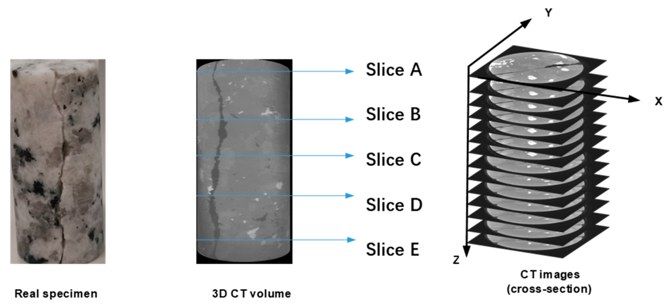
| Analysis Condition | CT Image Slice Number | Z-Direction (mm) | CT Image Slice Number | Z-Direction (mm) |
| Slice A | 161 | 2.7 | 161 | 2.7 |
| Slice B | 361 | 6.1 | 361 | 7.6 |
| Slice C | 661 | 9.9 | 661 | 13.9 |
| Slice D | 1261 | 18.9 | 1261 | 26.5 |
| Slice E | 1561 | 23.4 | 1561 | 32.8 |
| Mean Value of Rock σ1 | Mean Value of Void σ2 | Standard Distribution of Rock μ1 | Standard Distribution of Void μ2 | Tolerance T | Threshold |
|---|---|---|---|---|---|
| 118.6 | 4.5 | 29.5 | 8.6 | 33 | 85 |
Disclaimer/Publisher’s Note: The statements, opinions and data contained in all publications are solely those of the individual author(s) and contributor(s) and not of MDPI and/or the editor(s). MDPI and/or the editor(s) disclaim responsibility for any injury to people or property resulting from any ideas, methods, instructions or products referred to in the content. |
© 2024 by the authors. Licensee MDPI, Basel, Switzerland. This article is an open access article distributed under the terms and conditions of the Creative Commons Attribution (CC BY) license (https://creativecommons.org/licenses/by/4.0/).
Share and Cite
Song, C.; Li, T.; Li, H.; Huang, X. Application of Different Image Processing Methods for Measuring Rock Fracture Structures under Various Confining Stresses. Appl. Sci. 2024, 14, 9221. https://doi.org/10.3390/app14209221
Song C, Li T, Li H, Huang X. Application of Different Image Processing Methods for Measuring Rock Fracture Structures under Various Confining Stresses. Applied Sciences. 2024; 14(20):9221. https://doi.org/10.3390/app14209221
Chicago/Turabian StyleSong, Chenlu, Tao Li, He Li, and Xiao Huang. 2024. "Application of Different Image Processing Methods for Measuring Rock Fracture Structures under Various Confining Stresses" Applied Sciences 14, no. 20: 9221. https://doi.org/10.3390/app14209221
APA StyleSong, C., Li, T., Li, H., & Huang, X. (2024). Application of Different Image Processing Methods for Measuring Rock Fracture Structures under Various Confining Stresses. Applied Sciences, 14(20), 9221. https://doi.org/10.3390/app14209221