
Research on Coal and Rock Recognition in Coal Mining Based on Artificial Neural Network Models

Abstract
1. Introduction
2. Coal and Rock Image Acquisition and Image Feature Extraction
2.1. Collection of Coal Image and Rock Image Samples in Coal Mining Area
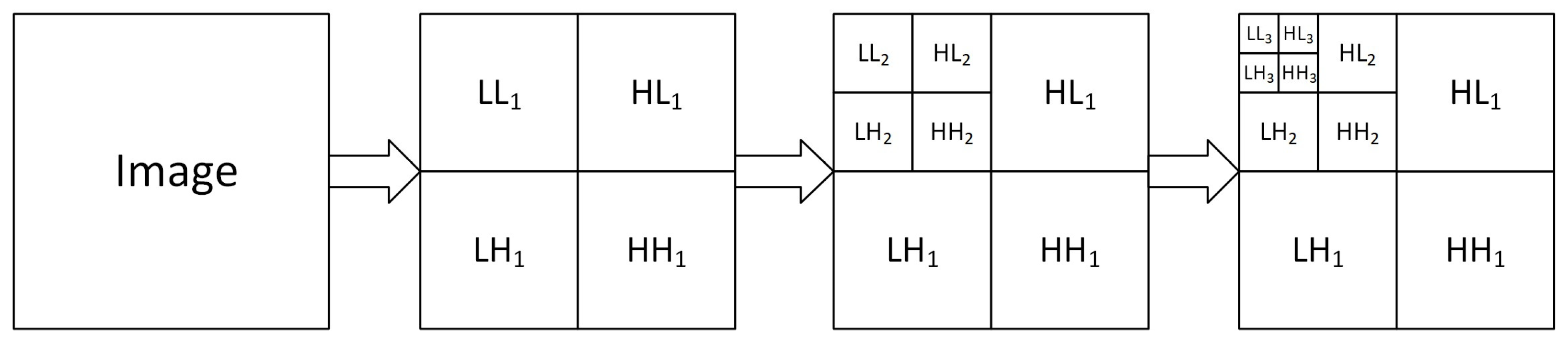
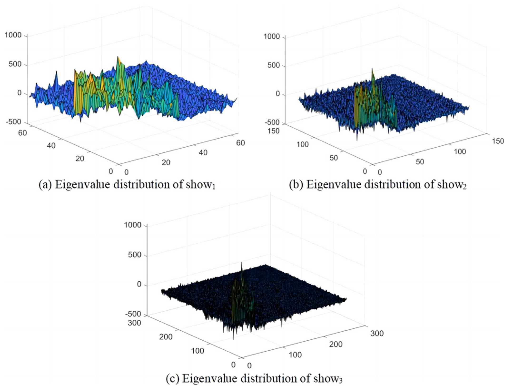
2.2. Image Feature Extraction Based on Wavelet Three-Level Decomposition
3. Coal and Rock Recognition Experiment Based on the BP Neural Network
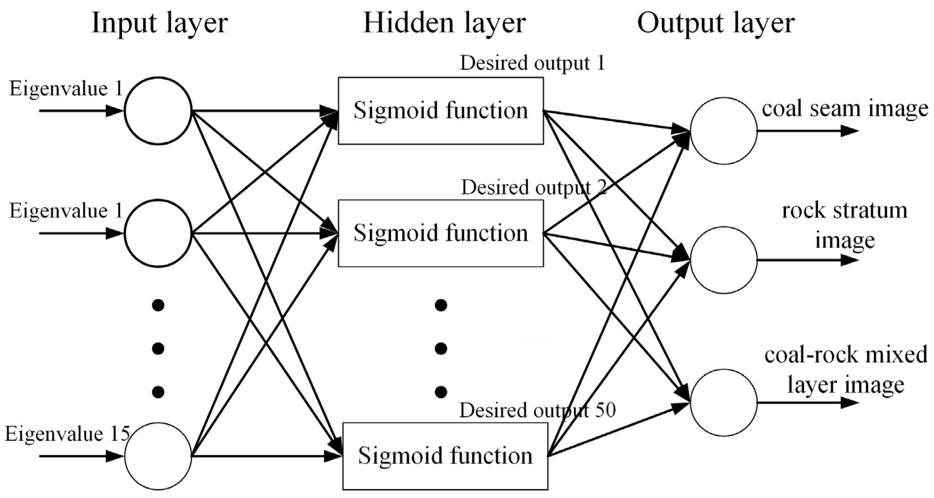
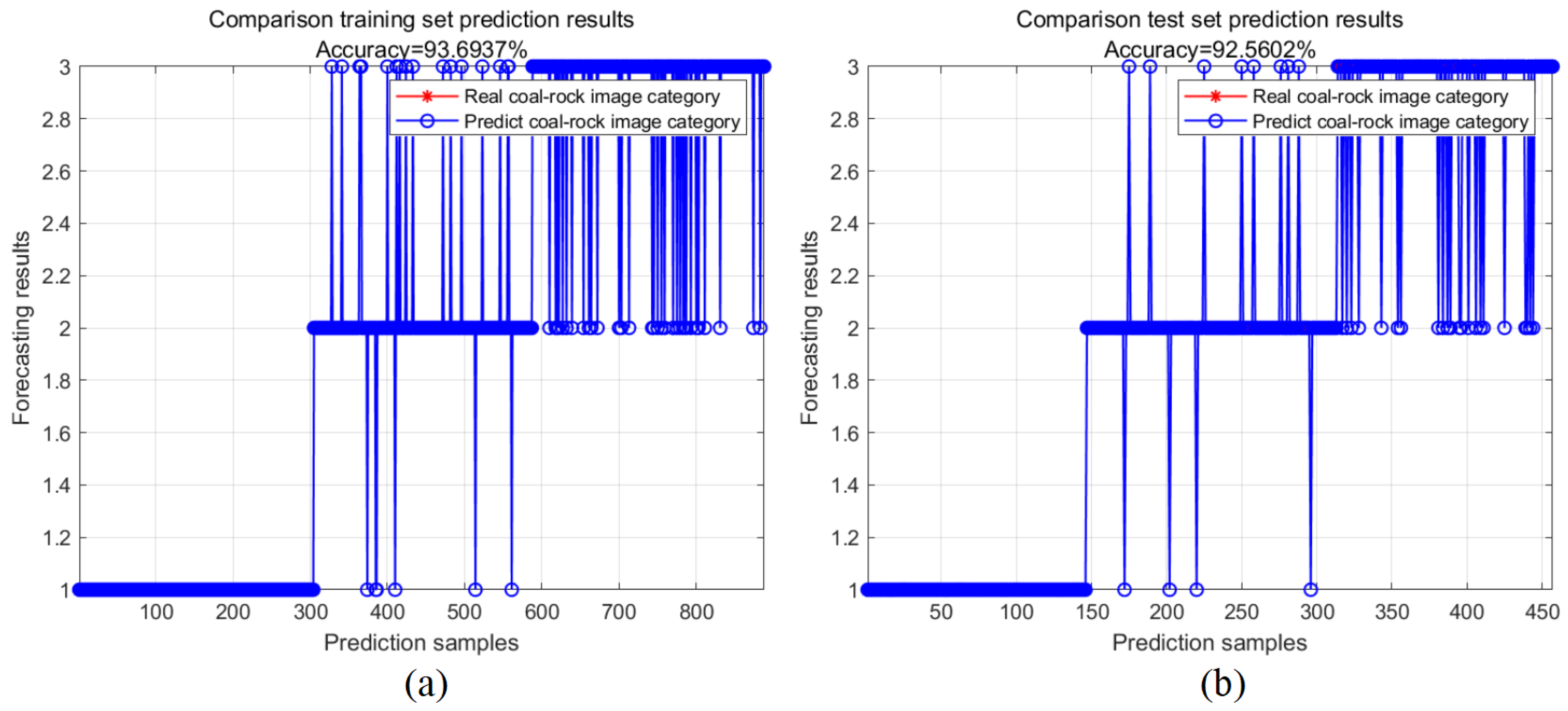
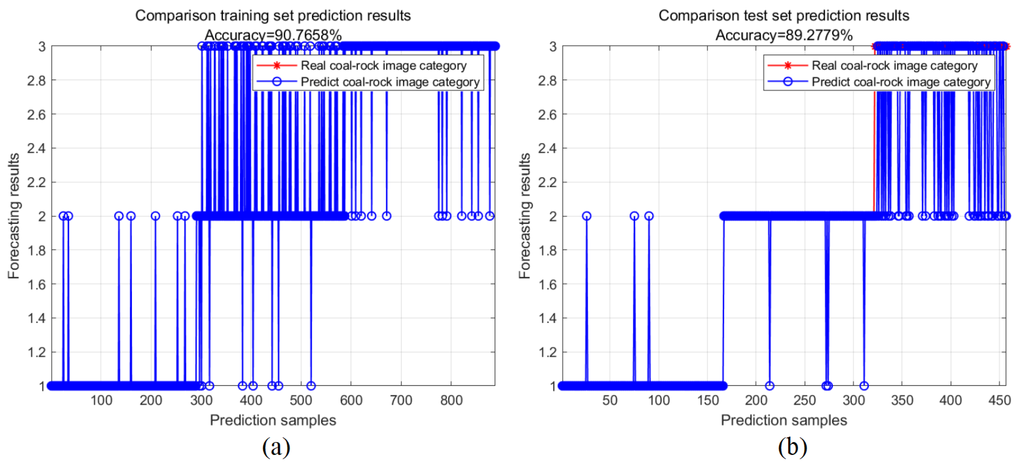
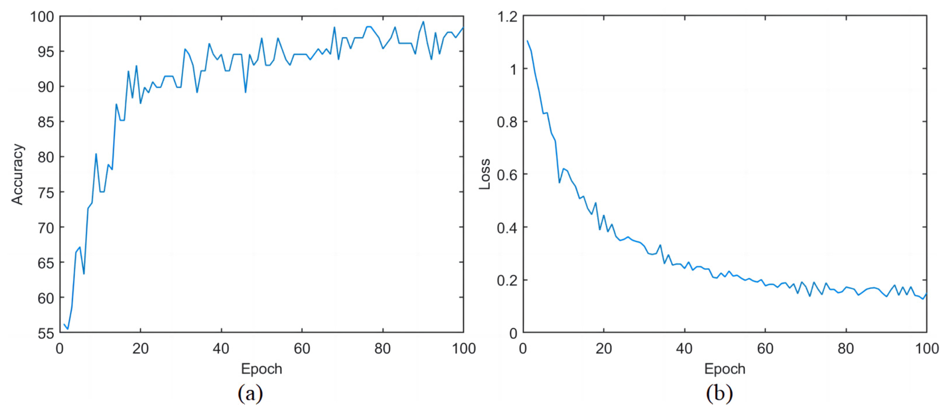
3.1. BP Neural Network Construction and Matlab Simulation Experiment
3.2. Control Group Experiment Based on Convolutional Neural Network
- (1)
- VGG16 network model
- (2)
- LeNet-5 network model
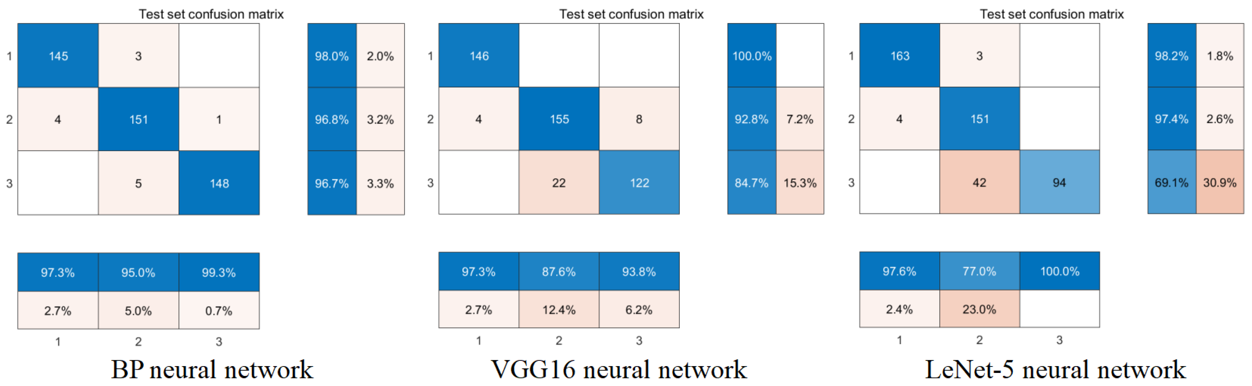
3.3. Performance Comparison of Network Models
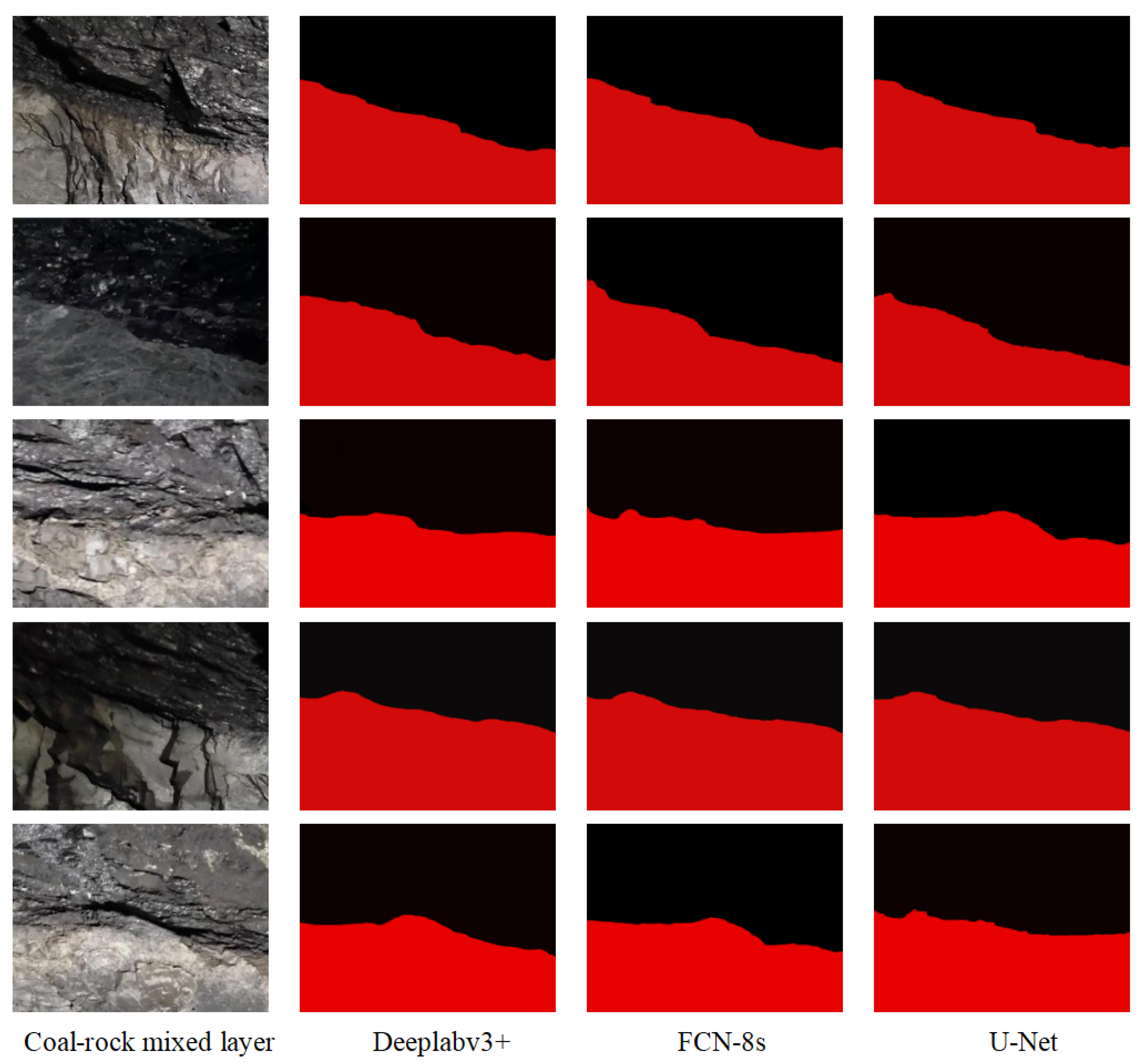
4. The Image Semantic Segmentation Experiment of the Coal–Rock Mixed Layer
5. Conclusions
Author Contributions
Funding
Institutional Review Board Statement
Informed Consent Statement
Data Availability Statement
Conflicts of Interest
References
- Wu, X.; Li, H.; Wang, B.; Zhu, M. Review on Improvements to the Safety Level of Coal Mines by Applying Intelligent Coal Mining. Sustainability 2022, 14, 16400. [Google Scholar] [CrossRef]
- Chen, W.; Jie, Z. New advances in automatic shearer cutting technology for thin seams in Chinese underground coal mines. Energy Explor. Exploit. 2021, 40, 3–16. [Google Scholar] [CrossRef]
- Wang, G.; Zhang, D. Innovation practice and development prospect of intelligent fully mechanized technology for coal mining. J. China Univ. Min. Technol. 2018, 47, 459–467. [Google Scholar]
- Wang, G. New development of longwall mining equipment based on automation and intelligent technology for thin seam coal. J. Coal Sci. Eng. 2013, 19, 97–103. [Google Scholar] [CrossRef]
- Sun, C.; Li, X.; Chen, J.; Wu, Z.; Li, Y. Coal-Rock Image Recognition Method for Complex and Harsh Environment in Coal Mine Using Deep Learning Models. IEEE Access 2023, 11, 80794–80805. [Google Scholar]
- Liu, C.; Jiang, J.; Jiang, J.; Zhou, Z.; Ye, S. Automatic Coal-Rock Recognition by Laser-Induced Breakdown Spectroscopy Combined with an Artificial Neural Network. Spectroscopy 2023, 38, 25–32. [Google Scholar]
- Gorai, A.K.; Raval, S.; Patel, A.K.; Chatterjee, S.; Gautam, T. Design and development of a machine vision system using artificial neural network-based algorithm for automated coal characterization. Int. J. Coal Sci. Technol. 2021, 8, 737–755. [Google Scholar] [CrossRef]
- Si, L.; Xiong, X.; Wang, Z.; Tan, C. A deep convolutional neural network model for intelligent discrimination between coal and rocks in coal mining face. Math. Probl. Eng. 2020, 2020, 2616510. [Google Scholar] [CrossRef]
- Gao, F.; Yin, X.; Liu, Q.; Huang, X.; Bo, Y.; Zhang, Q.; Wang, X. Coal-rock image recognition method for mining and heading face based on spatial pyramid pooling structure. J. China Coal Soc. 2021, 46, 4088–4102. [Google Scholar]
- Sun, C.M.; Wang, Y.P.; Wang, C.; Xu, R.J.; Li, X.E. Coal-rock interface identification method based on improved YOLOv3 and cubic spline interpolation. J. Min. Strat. Control. Eng. 2022, 4, 81–90. [Google Scholar]
- Fang, X.Q.; He, J.; Zhang, B.; Guo, M.J. Self-positioning system of the shearer in unmanned workface. J. Xi’an Univ. Sci. Technol. 2008, 28, 349–353. [Google Scholar]
- Chad, O.H.; James, C.A.; Ralston, J.C. Infrastructure-based localization of automated coal mining equipment. Int. J. Coal Sci. Technol. 2017, 4, 252–264. [Google Scholar]
- Yaghoobi, H.; Mansouri, H.; Farsangi, M.A.E.; Nezamabadi-Pour, H. Determining the fragmented rock size distribution using textural feature extraction of images. Powder Technol. 2019, 342, 630–641. [Google Scholar] [CrossRef]
- Wang, J.C.; Li, L.H.; Yang, S.L. Experimental study on gray and texture feature extraction of coal gangue image under different illumination. J. Coal Sci. Eng. 2018, 43, 3051–3061. [Google Scholar]
- Zhang, K.; Kang, L.; Chen, X.; He, M.; Zhu, C.; Li, D. A Review of Intelligent Unmanned Mining Current Situation and Development Trend. Energies 2022, 15, 513. [Google Scholar] [CrossRef]
- Wu, Q. Research on deep learning image processing technology of second-order partial differential equations. Neural Comput. Appl. 2023, 35, 2183–2195. [Google Scholar] [CrossRef]
- Daubechies, I. Ten Lectures on Wavelets. In CBMS-NSF Regional Conference Series in Applied Mathematics; Department of Mathematics, University of Lowell: Lowell, MA, USA; Society for Industrial and Applied Mathematics: Philadelphia, PA, USA, 2016. [Google Scholar]
- Haralick, R.M.; Shanmugam, K.; Dinstein, I.H. Textural features for image classification. IEEE Trans. Syst. Man Cybern. 1973, SMC-3, 610–621. [Google Scholar]
- Ha, V.K.; Ren, J.C.; Xu, X.Y.; Zhao, S.; Xie, G.; Masero, V.; Hussain, A. Deep Learning Based Single Image Super-resolution: A Survey. Int. J. Autom. Comput. 2019, 16, 413–426. [Google Scholar]
- Ying, C.; Huang, Z.; Ying, C. Accelerating the image processing by the optimization strategy for deep learning algorithm DBN. EURASIP J. Wirel. Commun. Netw. 2018, 2018, 232. [Google Scholar] [CrossRef]
- Luque, A.; Carrasco, A.; Martín, A.; de las Heras, A. The impact of class imbalance in classification performance metrics based on the binary confusion matrix. Pattern Recognit. 2019, 91, 216–231. [Google Scholar]
- Chicco, D.; Jurman, G. The advantages of the Matthews correlation coefficient (MCC) over F1 score and accuracy in binary classification evaluation. BMC Genom. 2020, 21, 6. [Google Scholar]
- Grandini, M.; Bagli, E.; Visani, G. Metrics for Multi-Class Classification: An Overview. arXiv 2020, arXiv:2008.05756. [Google Scholar]
- Tharwat, A. Classification assessment methods. Appl. Comput. Inform. 2021, 17, 168–192. [Google Scholar]
- Aouat, S.; Ait-hammi, I.; Hamouchene, I. A new approach for texture segmentation based on the Gray Level Co-occurrence Matrix. Multimed. Tools Appl. 2021, 80, 24027–24052. [Google Scholar] [CrossRef]
- Garcia-Garcia, A.; Orts-Escolano, S.; Oprea, S.; Villena-Martinez, V.; Rodríguez, J.G. A Review on Deep Learning Techniques Applied to Semantic Segmentation. arXiv 2017, arXiv:1704.06857. [Google Scholar]
- Wang, X.; Liu, F.; Ma, X. Mixed distortion image enhancement method based on joint of deep residuals learning and reinforcement learning. Signal Image Video Process. 2021, 15, 995–1002. [Google Scholar] [CrossRef]
- Reibman, A.R.; Bell, R.M.; Gray, S. Quality assessment for super-resolution image enhancement. In Proceedings of the 2006 International Conference on Image Processing, Atlanta, GA, USA, 8–11 October 2006; pp. 2017–2020. [Google Scholar]
- Zhou, H.; Hou, J.; Wu, W.; Zhang, Y.; Wu, Y.; Ma, J. Infrared and visible image fusion based on semantic segmentation. J. Comput. Res. Dev. 2021, 58, 436–443. [Google Scholar]
- Rahman, M.A.; Wang, Y. Optimizing Intersection-Over-Union in Deep Neural Networks for Image Segmentation. In Advances in Visual Computing; Bebis, G., Boyle, R., Parvin, B., Koracin, D., Porikli, F., Skaff, S., Entezari, A., Min, J., Iwai, D., Sadagic, A., et al., Eds.; Springer International Publishing: Cham, Switzerland, 2016; pp. 234–244. [Google Scholar]
- Shanbhag, A.G. Utilization of Information Measure as a Means of Image Thresholding. CVGIP Graph. Model. Image Process. 1994, 56, 414–419. [Google Scholar] [CrossRef]


| Feature Number | Coal Seam Characteristic Value | Rock Characteristic Value | Characteristic Value of Coal–Rock Mixed Layer |
|---|---|---|---|
| βLL (1) | 0.00983 | 0.0057 | 0.0038 |
| αLL (1) | 46.496 | 79.853 | 133.133 |
| GLL (1) | 0.0293 | 0.0368 | 0.0192 |
| ELL (1) | 119.345 | 144.28 | 219.836 |
| σLL (1) | 25.6 | 41.696 | 14.42 |
| βLL (2) | 0.014 | 0.00766 | 0.00375 |
| αLL (2) | 29.361 | 74.28 | 202.18 |
| GLL (2) | 0.0215 | 0.0193 | 0.0414 |
| ELL (2) | 221.5 | 255.691 | 301.225 |
| σLL (2) | 41.491 | 65.2 | 61.579 |
| βLL (3) | 0.0184 | 0.00977 | 0.0057 |
| αLL (3) | 101.577 | 139.641 | 369.682 |
| GLL (3) | 0.00681 | 0.00694 | 0.00607 |
| ELL (3) | 477.1 | 426.608 | 786.49 |
| σLL (3) | 70.662 | 89.390 | 59.581 |
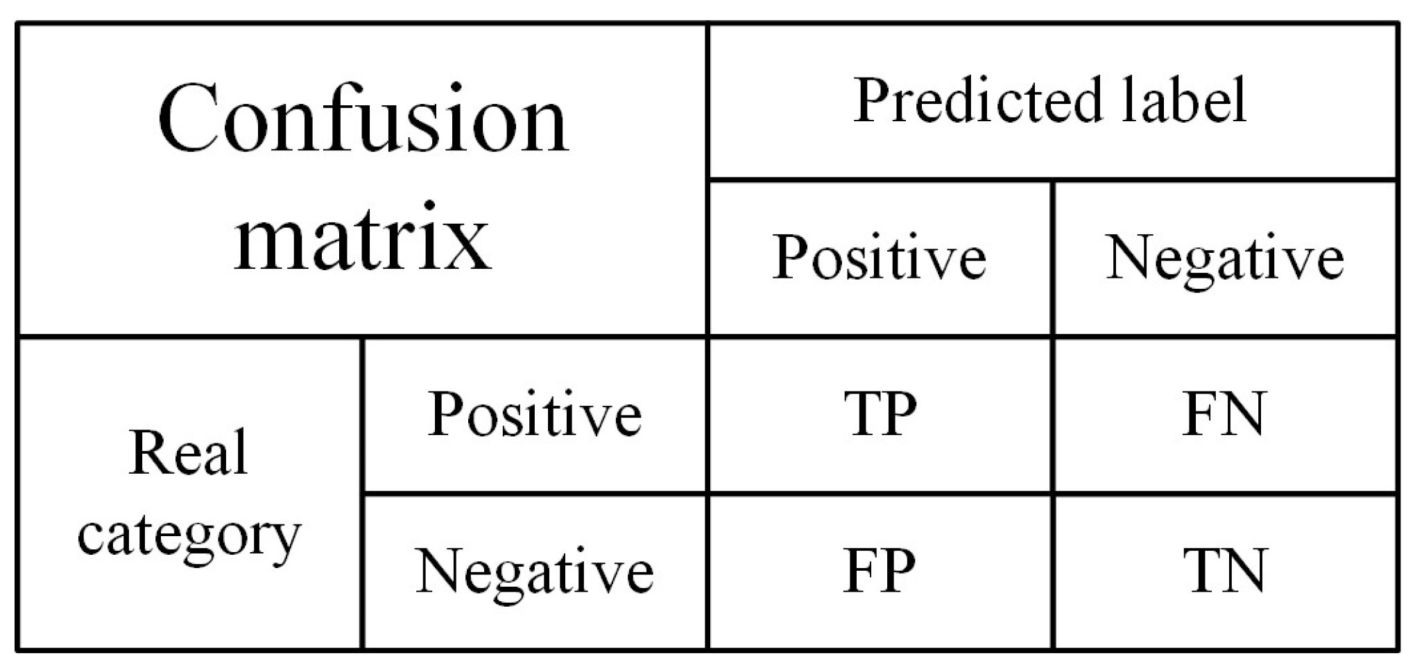
| Network Performance Evaluation Index | Computing Formula |
|---|---|
| Recall rate | |
| Accuracy rate | |
| Precision rate | |
| Specificity | |
| F1-score |
| Network Model Name | Accuracy Rate | Precision Rate | Recall Rate | Specificity | F1-Score |
|---|---|---|---|---|---|
| BP neural network | 97.16% | 95% | 96.7% | 96.32% | 95.84% |
| VGG16 network | 92.56% | 87.6% | 84.7% | 91% | 86.12% |
| LeNet-5 network | 89.28% | 77% | 69.91% | 89.27% | 73.29% |
| IOU | Deeplabv3+ | FCN-8s | U-Net |
|---|---|---|---|
| Sample 1 | 0.893 | 0.827 | 0.914 |
| Sample 2 | 0.945 | 0.893 | 0.961 |
| Sample 3 | 0.899 | 0.833 | 0.856 |
| Sample 4 | 0.914 | 0.876 | 0.910 |
| Sample 5 | 0.905 | 0.910 | 0.933 |
| …… | |||
| Sample 100 | 0.940 | 0.851 | 0.855 |
| Mean value | 0.912 | 0.860 | 0.891 |
Disclaimer/Publisher’s Note: The statements, opinions and data contained in all publications are solely those of the individual author(s) and contributor(s) and not of MDPI and/or the editor(s). MDPI and/or the editor(s) disclaim responsibility for any injury to people or property resulting from any ideas, methods, instructions or products referred to in the content. |
© 2024 by the authors. Licensee MDPI, Basel, Switzerland. This article is an open access article distributed under the terms and conditions of the Creative Commons Attribution (CC BY) license (https://creativecommons.org/licenses/by/4.0/).
Share and Cite
Sui, Y.; Zhang, L.; Sun, Z.; Yi, W.; Wang, M. Research on Coal and Rock Recognition in Coal Mining Based on Artificial Neural Network Models. Appl. Sci. 2024, 14, 864. https://doi.org/10.3390/app14020864
Sui Y, Zhang L, Sun Z, Yi W, Wang M. Research on Coal and Rock Recognition in Coal Mining Based on Artificial Neural Network Models. Applied Sciences. 2024; 14(2):864. https://doi.org/10.3390/app14020864
Chicago/Turabian StyleSui, Yiping, Lei Zhang, Zhipeng Sun, Weixun Yi, and Meng Wang. 2024. "Research on Coal and Rock Recognition in Coal Mining Based on Artificial Neural Network Models" Applied Sciences 14, no. 2: 864. https://doi.org/10.3390/app14020864
APA StyleSui, Y., Zhang, L., Sun, Z., Yi, W., & Wang, M. (2024). Research on Coal and Rock Recognition in Coal Mining Based on Artificial Neural Network Models. Applied Sciences, 14(2), 864. https://doi.org/10.3390/app14020864