An Iterative High-Precision Algorithm for Multi-Beam Array Stitching Method Based on Scanning Hartmann

Abstract

The multi-beam array stitching test system (MASTS) based on the Hartmann principle is employed to measure the aberrations in large-aperture optical systems. As each small-aperture and ideal parallel beam traverses the optical system, it is converged into a spot at the focal plane of the optical system. The centroid position of the spot contains the information about the wavefront slope of the sub-aperture at that specific location in the optical system. Scanning the optical system with this small-aperture beam across the entire aperture of the optical system, we can yield the aberration information to be tested. To mitigate pointing errors induced by scanning motion and accurately obtain the aberration signals of the optical system, nine beams are integrated into a 3 × 3 multi-beam array system, and their directions are aligned to be identical. However, achieving complete alignment in the same direction for all nine beams is a challenging task, resulting in errors due to their pointing differences within the array. This paper introduces an iterative algorithm designed to obtain high-precision multi-beam pointing errors and to reconstruct the wavefront of the optical system under test. This enables a more accurate measurement of wavefront aberrations in the optical system to be tested. Firstly, simulation models were implemented to validate the algorithm’s feasibility. Additionally, a scanning optical measurement system with a multi-beam array was developed in our lab, and the iterative algorithm was applied to process our experimental data. The results were then compared with interferometer data, demonstrating that our algorithm is feasible for MASTS to measure aberrations in large-aperture optical systems with high accuracy.

1. Introduction

Ground-based telescopes play a crucial role in astronomical observations, and their resolution capability determines the extent of the observable universe. To achieve higher imaging resolution and detection sensitivity, the apertures of ground-based telescopes are progressively increasing. The manufacturing and installation of large ground-based telescopes are an intricate process, where errors can significantly impact the quality of observations. The fabrication of large-aperture ground-based telescopes requires high standards in high-precision measurement technology. Testing for aberrations in the optical system is a pivotal aspect of the manufacturing process. The traditional methods for the aberration measurement in optical systems mainly involve the interferometric method. In this method, an interferometer is placed at the focal point of the optical system. The beam emitted from the interferometer passes through the optical system and reflects by a standard flat mirror, then returns along the same path into the interferometer. Using the analysis of interference patterns, the information about the aberrations in the optical system can be obtained [1,2]. It has the characteristics of simplicity, efficiency, and high accuracy. However, as the aperture of optical systems continues to increase, manufacturing the standard flat elements to match the aperture of the optical system becomes more difficult and expensive. The introduction of the sub-aperture stitching detection method addresses this issue by utilizing small-aperture flat elements to test the wavefront distribution of the sub-aperture of the system one by one. By using the wavefront consistency in the overlapping region of the sub-apertures as a constraint, the full-aperture aberrations of the optical system can be obtained. For example, the 3.5 m Herschel Space Telescope adopts the sub-aperture stitching method for system testing and achieves a final measurement accuracy of 400 nm [3,4]. The LOTIS (Large Optical Test and Integration Site) system, which has an aperture of 6.5 m, is tested using the sub-aperture stitching method with a movable 1.8 m flat mirror in diameter [5,6]. Researchers from the Xi’an Institute of Optics and Precision Mechanics, including Ke-Wei E, proposed a joint testing solution for a large-aperture off-axis optical system. This solution integrates the sub-aperture stitching test method with computer-assisted alignment technology and successfully achieves the assembly and testing of the primary and secondary mirror systems of AIMS (The Infrared System for the Accurate Measurement of Solar Magnetic Fields), intermediate focal systems, and visible light focal system [7,8]. The aberration testing of the primary mirror of the James Webb Space Telescope, with a diameter of 6.5 m, is conducted using an interferometer positioned at its center of curvature. During the integration testing of the system, the sub-aperture testing concept is applied by utilizing three flat mirrors with a size of 1.5 m each in diameter for full-aperture aberration testing [9,10,11,12]. Additionally, the aberration testing of the primary mirror utilizes the Hartmann testing method, where the light emitted from a point source located at the center of curvature of the main mirror is divided into multiple beams by the Hartmann screen. A Hartmann plate located near the focal point of the main mirror receives the focused spot array of the reflected light, and the centroid coordinates of each spot can be used to calculate the wavefront slope corresponding to the sub-aperture of the tested wavefront; thus, the full-aperture wavefront is reconstructed [13]. Wei et al. employed a multi-beam array scanning Hartmann method to detect the wavefront of a finished telescope [14,15,16]. The array integrated a 3 × 3 small-aperture parallel beam array as a measurement tool. In this method, the key factors which affect the test results are the multi-beam pointing errors (consistency errors within each tube in the array) and the array pointing errors (overall pointing deviation of the tube array at different positions during the scanning process). In Wei’s method, the pointing consistency between the 3 × 3 beams needs to be calibrated in advance. After obtaining all the measured array data, a correction quantity is applied to the beam pointing consistencies based on the assumption of small aberrations of the full-aperture optical system. However, when the samples of measurement data are limited, this method will still introduce significant testing errors. To address this issue, this paper proposes an iterative calculation algorithm that can simultaneously obtain the multi-beam pointing errors, the array pointing errors, and wavefront errors with high accuracy. The basic principles of the algorithm are described and verified through simulation calculations firstly. Based on this, a testing system is developed, and experimental comparisons are conducted to validate the feasibility of the proposed algorithm.

2. Methods

The principle of MASTS is illustrated in Figure 1a. The parallel beams with a small aperture emitted from the multi-beam array system pass through the optical system to be tested. The CCD camera, positioned at the focal plane of the system, captures the formed spots when the beams are focused by the optical system, which consists of a primary mirror and a secondary mirror. The wavefront slope information of the measured sub-aperture in the optical system can be calculated from the centroid coordinates of the focal spots. The multi-beam array system integrates 3 × 3 small-aperture collimator tubes that are maintained in the same direction to make their output beam parallel. The multi-beam array then scans through the entire aperture of the optical system under test to obtain its slopes’ information. The full-aperture aberration of the optical system is subsequently reconstructed using a wavefront reconstruction algorithm [17,18,19]. One of the scanning paths is shown in Figure 1b, where the numbers indicate the identification of each sub-beam in the multi-beam array system, and the arrows indicate the scanning path of it.

During actual measurements, the posture of the multi-beam array system is not stable as it moves along the scanning path. This instability can lead the changes in the orientation of the multi-beam array after movement. Furthermore, aligning the individual sub-beams in the multi-beam array system strictly along the same orientation is not feasible. In this paper, using beam No. 5 as a reference, the centroid coordinate of the spot formed after the focusing of a certain beam by the optical system can be expressed as

$$\left\{\begin{array}{c}{C}_{j,x}=D_{j,x}+{\Delta }_x+E_{j,x}\\ C_{j,y}=D_{j,y}+{\Delta }_y+E_{j,y}\end{array}\right., \mathrm{where}\left\{\begin{array}{c}{E}_{5,x}=0\\ E_{5,y}=0\end{array}\right.$$

(1)

where the subscripts j, x, and y represent the sub-beam number in the array and the corresponding coordinates of the centroid in the x and y directions, respectively. The symbol ‘C’, which are the actual test data, represents the centroid coordinates of the spot. The symbol ‘D’, which represents the sub-aperture wavefront slope information, denotes the centroid offset component of the beam caused by the sub-aperture aberration of the tested system. The symbol ‘Δ’ represents the centroid offset component caused by the scanning motion-induced array pointing error. The symbol ‘E’ is the centroid offset component caused by multi-beam pointing errors. After neglecting the ‘E’, both sides of Equation (1) are divided by the focal length f of the optical system, and the slope expression can be written as

$$\left\{\begin{array}{c}{M}_x=S_x+T_x\\ M_y=S_y+T_y\end{array}\right.$$

(2)

In Equation (2), M, S, and T correspond to the slopes of ‘C’, ‘D’, and ‘Δ’ in Equation (1), respectively. Slope S can be expressed using Zernike polynomials:

$$\left\{\begin{array}{c}{S}_x=c_1\frac{\partial Z_1(x,y)}{\partial x}+c_2\frac{\partial Z_2(x,y)}{\partial x}+\dots +c_m\frac{\partial Z_m(x,y)}{\partial x}\\ S_y=c_1\frac{\partial Z_1(x,y)}{\partial y}+c_2\frac{\partial Z_2(x,y)}{\partial y}+\dots +c_m\frac{\partial Z_m(x,y)}{\partial y}\end{array}\right.$$

(3)

Solving Equations (2) and (3) simultaneously, we obtain

$$\left\{\begin{array}{c}{M}_x=c_1\frac{\partial Z_1(x,y)}{\partial x}+c_2\frac{\partial Z_2(x,y)}{\partial x}+\dots +c_m\frac{\partial Z_m(x,y)}{\partial x}+T_x\\ M_y=c_1\frac{\partial Z_1(x,y)}{\partial y}+c_2\frac{\partial Z_2(x,y)}{\partial y}+\dots +c_m\frac{\partial Z_m(x,y)}{\partial y}+T_y\end{array}\right.$$

(4)

The measurement data obtained at each sampling point on the optical system for each small beam are represented by Equation (4). The measurement data obtained by all small-aperture beams at all sampling positions can be expressed in matrix form, as follows:

$$\left[\begin{array}{cccccccccccc}\partial Z_{1,1}/\partial x& \partial Z_{1,2}/\partial x& \dots & \partial Z_{1,term}/\partial x& 1& \dots & 0& 0& 0& \dots & 0& 0\\ \partial Z_{2,1}/\partial x& \partial Z_{2,2}/\partial x& \dots & \partial Z_{2,term}/\partial x& 1& \dots & 0& 0& 0& \dots & 0& 0\\ ⋮& ⋮& \dots & ⋮& ⋮& \dots & ⋮& 0& ⋮& \dots & ⋮& 0\\ \partial Z_{n,1}/\partial x& \partial Z_{n,2}/\partial x& \dots & \partial Z_{n,term}/\partial x& 0& \dots & 0& 1& 0& \dots & 0& 0\\ \partial Z_{1,1}/\partial y& \partial Z_{1,2}/\partial y& \dots & \partial Z_{1,term}/\partial y& 0& \dots & 0& 0& 1& \dots & 0& 0\\ \partial Z_{2,1}/\partial y& \partial Z_{2,2}/\partial y& \dots & \partial Z_{2,term}/\partial y& 0& \dots & 0& 0& 1& \dots & 0& 0\\ ⋮& ⋮& \dots & ⋮& ⋮& \dots & ⋮& 0& ⋮& \dots & ⋮& ⋮\\ \partial Z_{n,1}/\partial y& \partial Z_{n,2}/\partial y& \dots & \partial Z_{n,term}/\partial y& 0& \dots & 0& 0& 0& \dots & 0& 1\end{array}\right]·\left[\begin{array}{c}Cof{f}_1\\ Cof{f}_2\\ ⋮\\ Cof{f}_{term}\\ T_{1x}\\ T_{2x}\\ ⋮\\ T_{mx}\\ T_{1y}\\ T_{2y}\\ ⋮\\ T_{my}\end{array}\right]=\left[\begin{array}{c}{M}_{x,1}\\ M_{x,2}\\ \dots \\ M_{x,term}\\ M_{y,1}\\ M_{y,2}\\ ⋮\\ M_{y,term}\end{array}\right]$$

(5)

In Equation (5), the symbol ‘Coff’ represents the Zernike coefficients of the wavefront aberration for the optical system, and the symbol ‘T’ represents the slope associated with ‘Δ’. By applying the least squares method to solve Equation (5), the values of ‘T’ and ‘Coff’ can be accurately calculated. If the magnitude of ‘E’ is too large to be ignored, the ‘Coff’ obtained from Equation (5) will be incorrect with significant astigmatism. Therefore, this paper proposes an iterative method to first obtain the multi-beam pointing error and then compensate it into the test data to eliminate the influence of ‘E’ on the reconstructed wavefront. For example, let us consider a large-aperture optical system with an RMS value of aberration better than 0.08 λ and a focal length of 8 m. In this system, a 50 mm sized sub-aperture aberration at any position causes the centroid coordinate shift ‘D’ at the focal plane to be less than 0.5 μm, which is much smaller than the quantities of ‘E’ and ‘Δ’. Therefore, the ‘D’ in Equation (1) can be temporarily ignored, and the centroid data obtained for all sub-apertures are written in matrix form, as follows:

$$\left[\begin{array}{cccccccccccccccc}1\hfill & \dots \hfill & 0\hfill & 0\hfill & 0\hfill & \dots \hfill & 0\hfill & 0\hfill & 0\hfill & \dots \hfill & 0\hfill & 0\hfill & 0\hfill & \dots \hfill & 1\hfill & 0\hfill \\ 1\hfill & \dots \hfill & 0\hfill & 0\hfill & 0\hfill & \dots \hfill & 0\hfill & 0\hfill & 0\hfill & \dots \hfill & 0\hfill & 0\hfill & 0\hfill & \dots \hfill & 0\hfill & 1\hfill \\ ⋮\hfill & \dots \hfill & ⋮\hfill & 0\hfill & ⋮\hfill & \dots \hfill & ⋮\hfill & ⋮\hfill & ⋮\hfill & \dots \hfill & ⋮\hfill & 0\hfill & ⋮\hfill & \dots \hfill & 0\hfill & 0\hfill \\ 0\hfill & \dots \hfill & 0\hfill & 1\hfill & 0\hfill & \dots \hfill & 0\hfill & 0\hfill & 0\hfill & \dots \hfill & 0\hfill & 1\hfill & 0\hfill & \dots \hfill & 0\hfill & 0\hfill \\ 0\hfill & \dots \hfill & 0\hfill & 0\hfill & 1\hfill & \dots \hfill & 0\hfill & 0\hfill & 0\hfill & \dots \hfill & 0\hfill & 0\hfill & 1\hfill & \dots \hfill & 0\hfill & 0\hfill \\ 0\hfill & \dots \hfill & 0\hfill & 0\hfill & 1\hfill & \dots \hfill & 0\hfill & 0\hfill & 1\hfill & \dots \hfill & 0\hfill & 0\hfill & 0\hfill & \dots \hfill & 0\hfill & 0\hfill \\ ⋮\hfill & \dots \hfill & ⋮\hfill & 0\hfill & ⋮\hfill & \dots \hfill & ⋮\hfill & ⋮\hfill & 0\hfill & \dots \hfill & 0\hfill & 0\hfill & 0\hfill & \dots \hfill & 0\hfill & 0\hfill \\ 0\hfill & \dots \hfill & 0\hfill & 0\hfill & 0\hfill & \dots \hfill & 0\hfill & 1\hfill & 0\hfill & \dots \hfill & 1\hfill & 0\hfill & 0\hfill & \dots \hfill & 0\hfill & 0\hfill \end{array}\right]·\left[\begin{array}{c}{\Delta }_{1x}\\ {\Delta }_{2x}\\ ⋮\\ {\Delta }_{mx}\\ {\Delta }_{1y}\\ {\Delta }_{2y}\\ ⋮\\ {\Delta }_{my}\\ E_{1x}\\ E_{2x}\\ E_{3x}\\ \begin{array}{c}⋮\\ E_{9x}\\ E_{1y}\\ E_{2y}\\ E_{3y}\\ ⋮\\ E_{8y}\\ E_{9y}\end{array}\end{array}\right]=\left[\begin{array}{c}{C}_{x,1}\\ C_{x,2}\\ ⋮\\ C_{x,term}\\ C_{y,1}\\ C_{y,2}\\ ⋮\\ C_{y,term}\end{array}\right]$$

(6)

By applying the least squares method to solve Equation (6), the value of E can be determined. However, since the calculation process neglects D, the obtained value for E in this instance is denoted as $E_{near}$, which is an approximation to E. The accuracy of the computed value of E can be improved through the following iterative calculations.

The iterative process is illustrated in Figure 2. The notation with the subscript “near” represents an approximation with errors, while the notation without subscripts represents the actual values. The iterative steps are as follows:

• Since D is ignored, E solved by Equation (6) is not accurate enough and can be represented as $E_{near}$, as mentioned above. Then, the $E_{near}$ is subtracted from the original measurement data to obtain the data processed first.
• The data processed first are plugged into Equation (5) to solve for an approximate wavefront. With this approximate wavefront, the approximate $D_{near}$ is calculated, which represents the sub-aperture aberration signal. The $D_{near}$ is subtracted from the original measurement data to obtain the data processed second.
• The data processed second are plugged into Equation (6) to obtain a more accurate $E_{near}$.

Figure 2. Iterative process flowchart.

Figure 2. Iterative process flowchart.

By iterating through these steps, continually updating E and D, the process is repeated until the relative change in D is less than a threshold, which is set for simulations in this paper as 0.0055 μm.

3. Simulations

A Gregorian optical system model with an optical system aperture of 1 m and a focal length of 8 m is established in optical design software, as depicted in Figure 3a. The optical system aberration is illustrated in Figure 3b, and its Zernike coefficients are presented in

Table 1. The standard Zernike coefficients for the aberration illustrated in Figure 3b.

Standard Zernike Terms	Coefficients
Z4	−0.003 λ
Z5	0.0155 λ
Z6	−0.0152 λ
Z7	−0.0124 λ
Z8	0.0124 λ
Z9	0.00 λ
Z10	0.0122 λ

. This paper utilizes the image simulation function in optical design software to generate images of all small-aperture beams focused by the optical system. Through collaborative simulation between programming software and optical design software, interaction between the two is achieved using the Dynamic Link Library (DLL) pyzdde [20], programming software that plans the sampling positions of the beams and sends commands. Optical design software receives the commands, executes them, and outputs spot images corresponding to the sampled beams to a specified folder. Subsequently, programming software reads these spot images and calculates their centroids. In order to simulate the array pointing errors caused by scanning motion, different field-of-view angles are set for nine beams at various measurement positions of the array system, as illustrated in Figure 4. Additionally, multi-beam pointing errors are simulated by assigning different field-of-view angles to the beams with different numbers. Measured using an auto-collimating way in our lab, the array pointing error angle caused by scanning motion ranges from 6 to 9 arcseconds, and after a rough calibration, the aligned pointing error angle between the nine beams ranges from 8 to 12 arcseconds, which are random. The magnitudes of the array pointing error and multi-beam pointing error are plugged into the simulation.

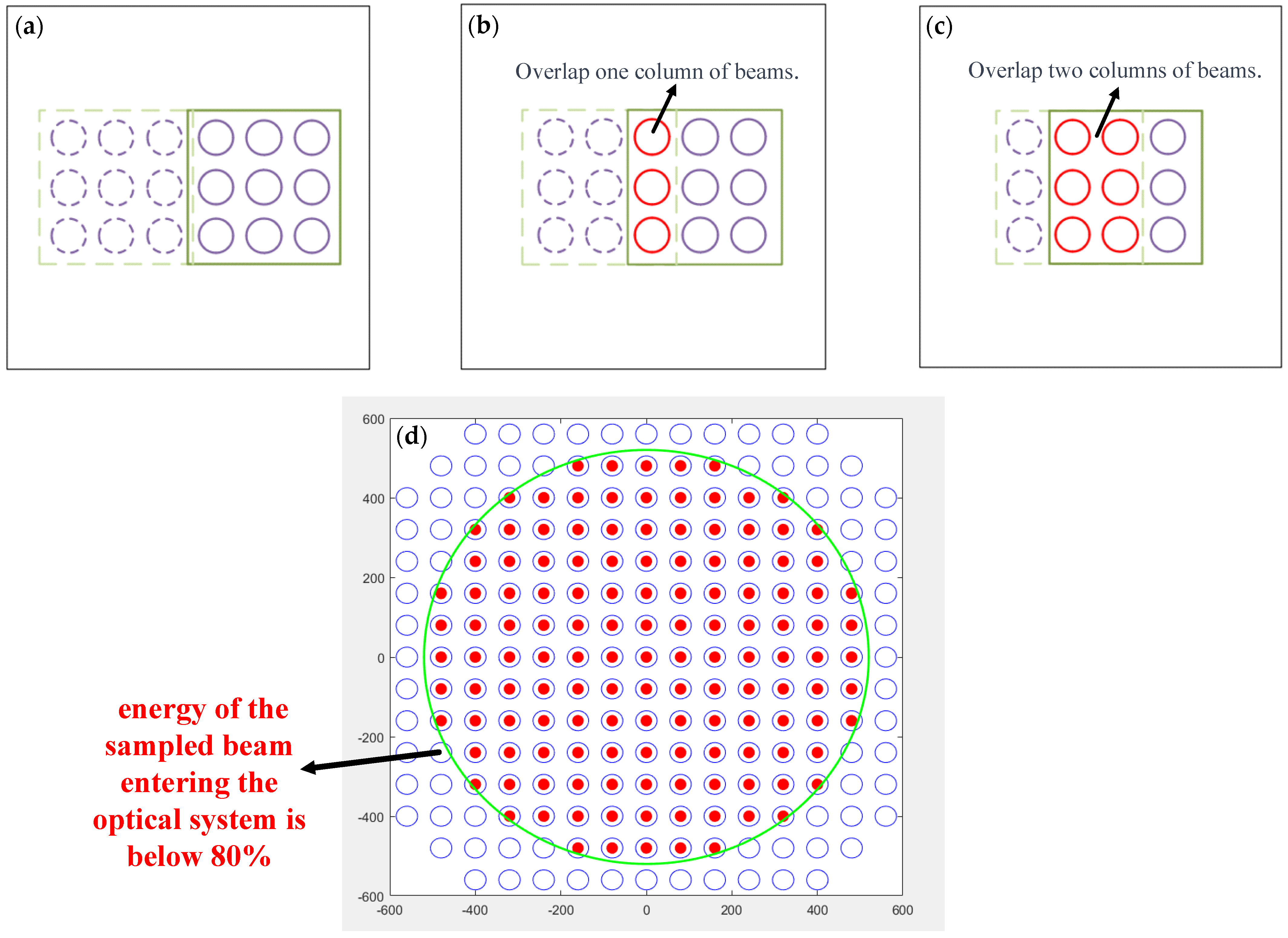
Additionally, the scanning way of the multi-beam array system is designed with three kinds of steps, as shown in Figure 4a–c, the scanning path of it for the full-aperture sampling using the multi-beam array system is illustrated in Figure 1b, and the distribution of all sampled points is shown in Figure 4d. Points sampled at the edge of the optical system aperture are considered effective sampled points when the energy of their beams entering the optical system reaches 80% of the total beam energy. When a higher wavefront measurement resolution is required, smaller step sizes can be considered to increase sampling density. However, as the step size decreases, the sampled data increase, which will cause a rapid decline in measurement efficiency. Therefore, it is essential to choose an appropriate step size based on the requirements of accuracy and efficiency.

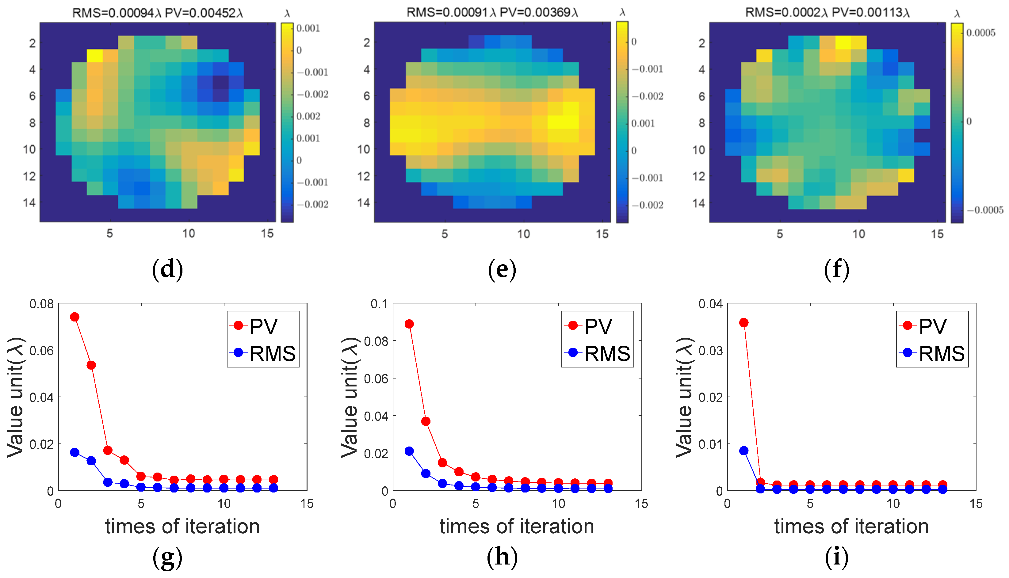
Due to the use of a significant number of random values in the simulation, the process is repeated 1000 times. The average of all results is taken as the final simulation result. When the array scans with different step sizes, the iterative method yields the following results in Figure 5.

From Figure 5, it can be seen that the RMS values of the residual aberration obtained using the iterative method are all less than one-thousandth of a wavelength after the reconstructed wavefront is subtracted from the known aberration distribution. The RMS value shown in Figure 5c approaches one-ten-thousandth of a wavelength, which demonstrates the accuracy of the iterative method in simulation results. As the array scanning step size decreases, the aberration obtained through the iterative method becomes closer to the known aberration. Stated differently, reducing the step size enhances the accuracy of the iterative method and reduces the number of iterations needed for convergence. This is attributed to the fact that a smaller scanning step size brings adjacent measurement positions of the multi-beam array closer, resulting in a denser sampling of beams. As a consequence, more data are collected, and a larger dataset implies more accurate fitting results for Equations (5) and (6). 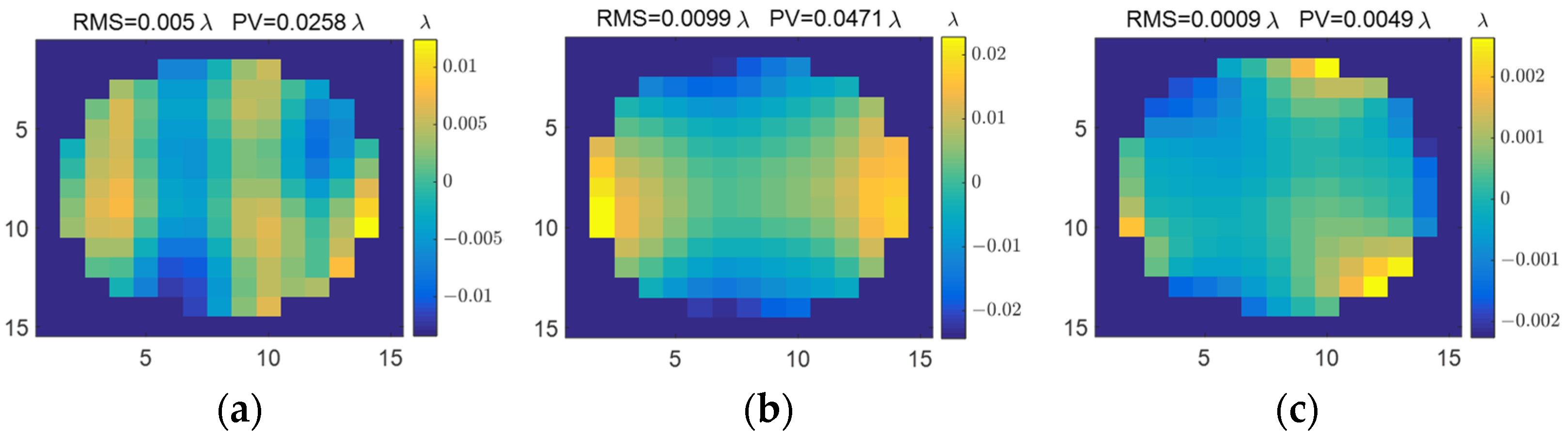Additionally, the averaging method proposed in reference [16] assumes the wavefront in the optical system is uniformly sampled by an individual beam. It calculates the average of a large amount of multi-beam pointing error data based on statistical principles to eliminate sub-aperture aberration signals. But, a larger reconstruction error will be induced. The residuals after subtracting the reconstructed wavefront distribution using the averaging method from the preset aberrations are shown in Figure 6.

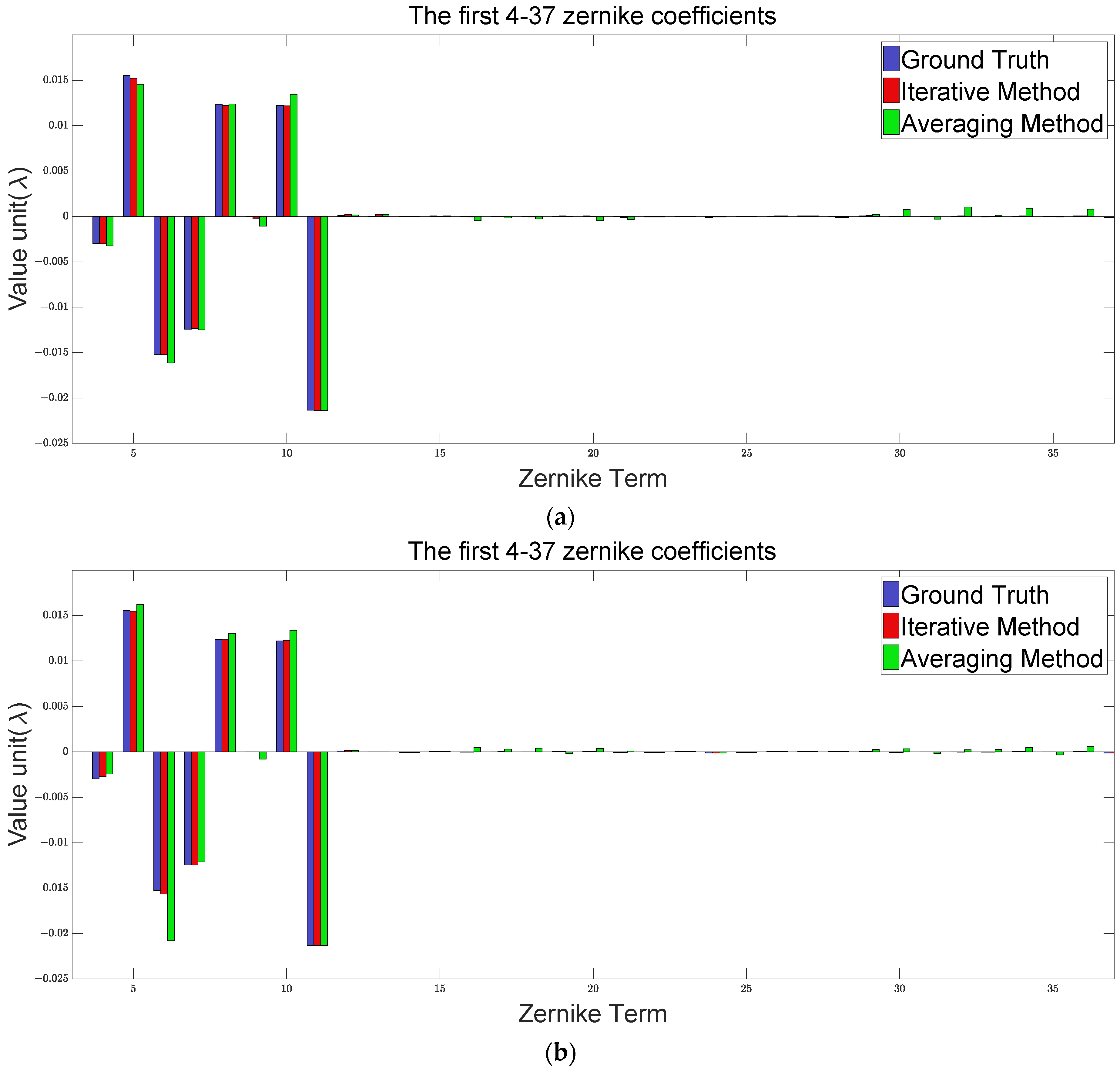
Under the same conditions, the residuals of the iterative method are significantly smaller than those of the averaging method, as shown in Figure 6. Figure 7 illustrates the comparison among the ground truth of aberration, the result using the iterative method, and the result using the averaging method with the coefficients of Zernike polynomial.

From Figure 7, it can be seen that the Zernike coefficients of the reconstructed wavefront using the two methods exhibit errors in the lower-order terms, particularly evident in the fifth and sixth terms (astigmatism). Conversely, the high-order Zernike coefficients show a similar trend. This corresponds well with the extensive simulation results we conducted. In summary, with different scanning step sizes, the results obtained through the iterative method exhibit a clear advantage over those obtained through the averaging method.

4. Experiments

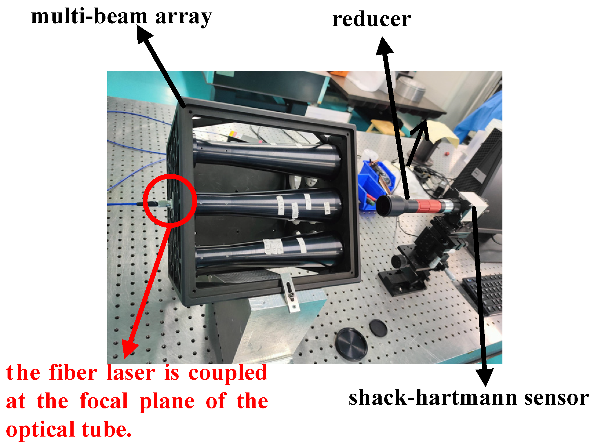
The beams emitted by the multi-beam array system developed in our lab have a wavelength of 632.8 nm and a beam size of 50 mm in diameter. The interval of adjacent beams in the multi-beam array system is 80 mm. Guided by the Shack–Hartmann wavefront sensor in the setup as shown in Figure 8, we achieved a wavefront error of less than 0.02 λ RMS for each collimator beam in the multi-beam array system. The laser is a single-mode fiber-coupled laser with a fiber output power exceeding 10 mW. Some characteristics of the Shack–Hartmann sensor are presented in

Table 2. The characteristics of Shack–Hartmann sensor.

Size of a Micro Lens	Micro Lens Focal Length	Micro Lens Array Resolution	CCD Pixel Size	Measurement Frame Rate
0.3 × 0.3 mm	15 mm	45 × 60	5.5 μm	15 Hz

. Note that the beam size, with a diameter of 50 mm, emitted by the multi-beam array, is reduced through a reducer to match the field of view of the Shack–Hartmann wavefront sensor.

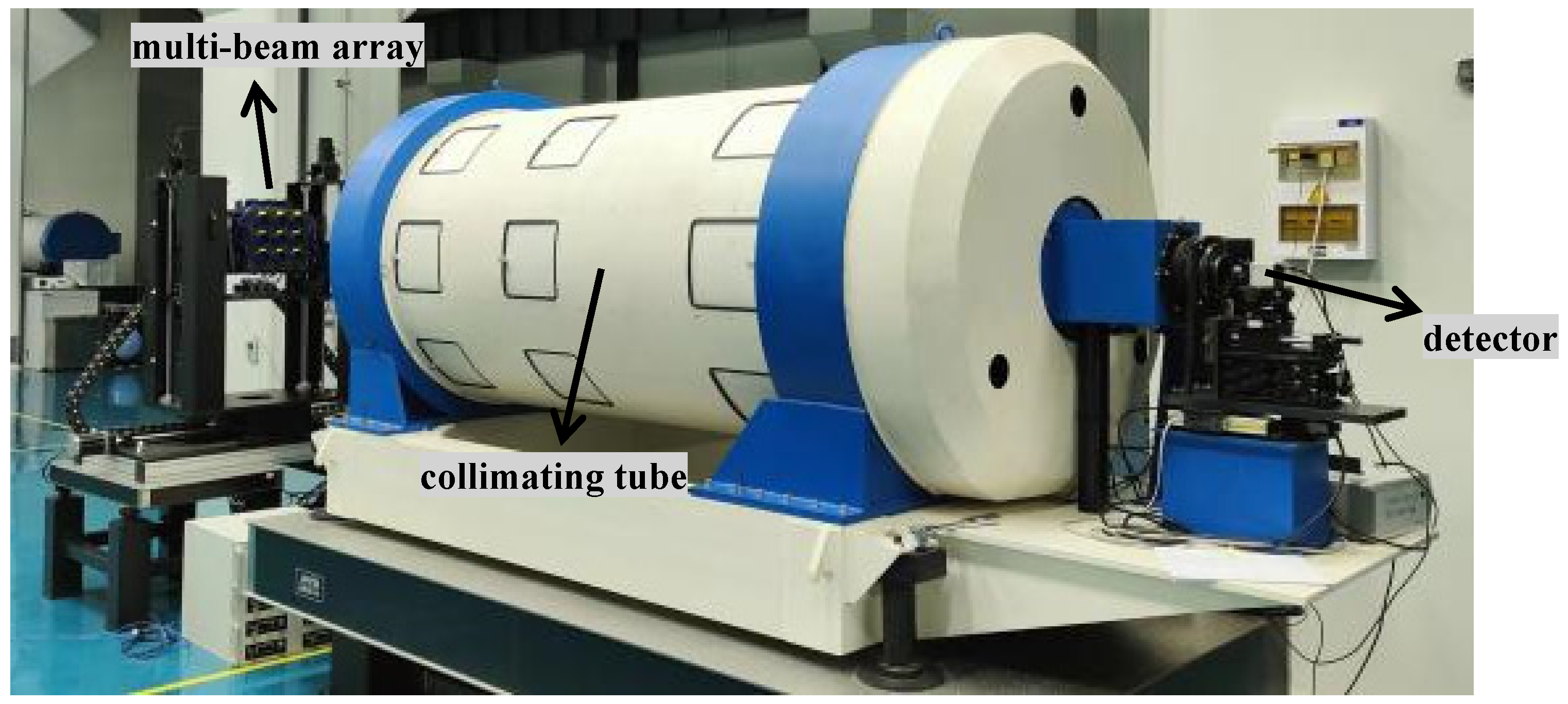
Next, a Cassegrain-type collimating tube with a focal length of 20 m is employed to align the nine beams in the same direction, as shown in Figure 9. Each beam of the multi-beam array system is sequentially focused on the CCD using the collimating tube. We adjust the nine focal spots to align as closely as possible at the same position. However, due to the limitations of mechanism, the centroids of the spots did not exactly coincide at the same coordinates.

Afterward, the setup for aberration measurement of the optical system is established, as shown in Figure 10b. The optical system has a focal length of 8 m with an aperture diameter of 560 mm. The testing procedure is outlined as follows:

• Align the central beam (No. 5) of the multi-beam array with the optical system’s aperture center, which is used as the coordinate system origin. Determine coordinates for all measurement positions based on the optical system’s aperture size and the array scanning step size.
• Drive the multi-beam array along a two-dimensional guide to the positions determined in Step 1. Sequentially illuminate the beams according to their numerical order. Illuminate each beam for one second to stabilize spot images. Subsequently, the detector captures the image. After completing measurements at the current position, move the multi-beam array system to the next measurement position. Repeat Steps 1 and 2 until all positions within the optical system’s aperture are covered.

Figure 10. Experimental setup of (a) multi-beam array and (b) MASTS.

Figure 10. Experimental setup of (a) multi-beam array and (b) MASTS.

In summary of the above experiments, firstly, we accomplished the integrated installation of a multi-beam array that utilizes Hartmann wavefront sensors for real-time wavefront detection, guiding the coupling of fiber lasers. Next, we employed a long-focal-length collimating tube for the calibration and testing of the alignment consistency of a multi-beam array. Finally, we tested the wavefront of the optical system using the MASTS. 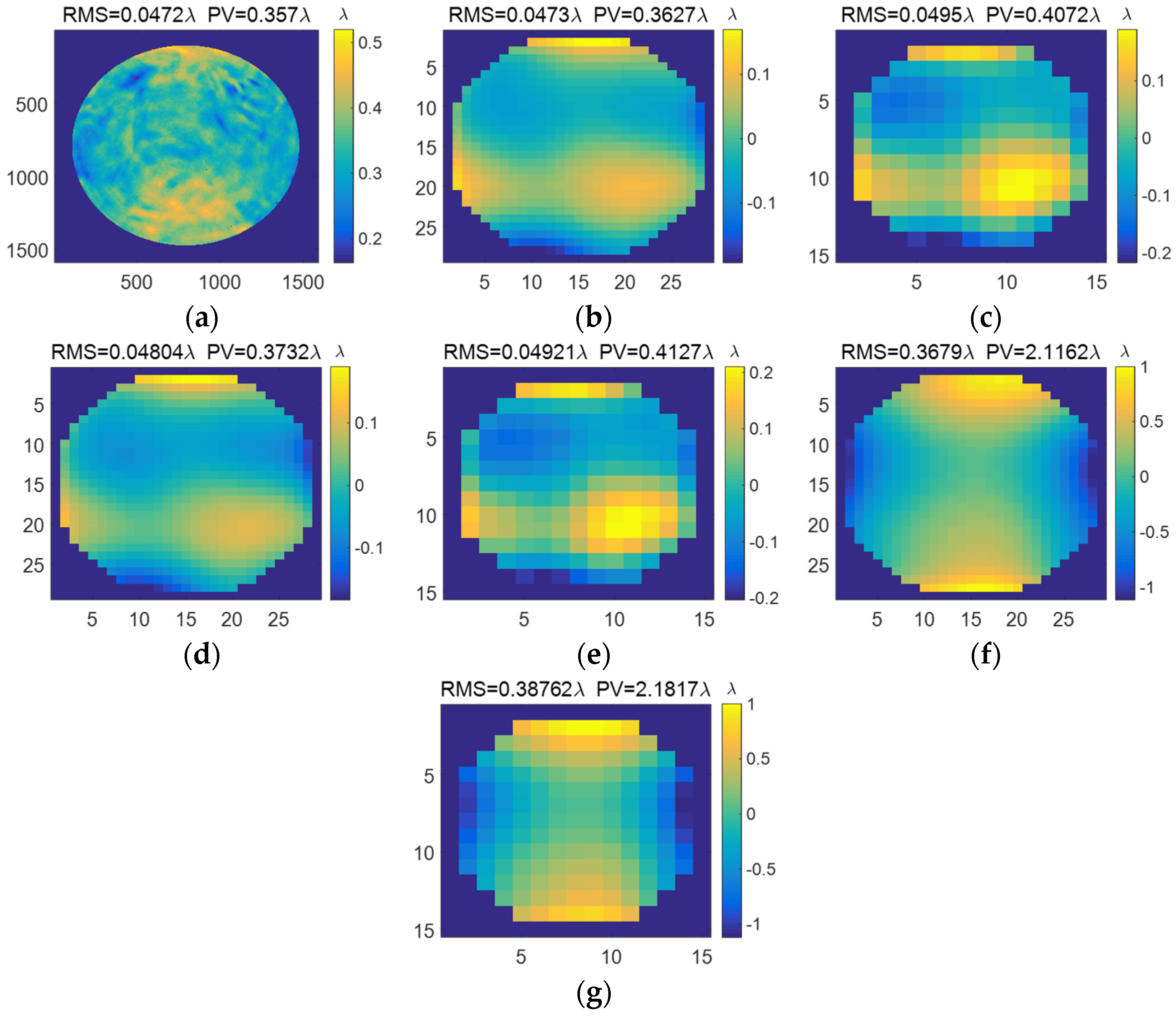The test results of the experimental measurement are illustrated in Figure 11.

As shown in Figure 11, it can be seen that the root mean square (RMS) value obtained through the iterative method differs by less than 0.0001 $\lambda$ from the RMS value of the interferometer data, which indicates the accuracy and correctness of the iterative approach. The RMS values of the reconstruction with a 20 mm step size are closer to the interferometer test results compared with the 40 mm step size. This is because with a smaller step size in the array motion, the beam sampling of the optical system becomes more densely distributed. As a result, the reconstructed wavefront has a higher resolution. A higher wavefront resolution implies more accurate calculations of wavefront aberrations, leading to more accurate PV and RMS values. Certainly, choosing an even smaller motion step size can provide a higher resolution wavefront and consequently more accurate data. However, the data shown in Figure 11b are already comparable to interferometer data. Opting for a smaller motion step size would extend the testing time to over 3 h. Comparing the results of the iterative method with the averaging method, it shows that under the 20 mm step size condition, the RMS values from the iterative method are closer to the interferometer data. Under the 40 mm step size condition, the averaging method yields an RMS value slightly closer to the interferometer data than the iterative method. This discrepancy may be attributed to insufficient wavefront resolution, causing minor errors in the RMS value calculations. In terms of RMS value calculations, the iterative reconstruction results are superior to the averaging reconstruction results. The wavefront distributions reconstructed under different motion step sizes exhibit high repeatability for the array. Figure 11f,g demonstrate that if multi-beam pointing errors are not compensated for, directly plugging raw test data into Equation (5) will result in incorrect reconstruction. This highlights the necessity of using our method to handle MASTS test data. The differences in the wavefront distribution between MASTS test results and interferometric test results may be attributed to the fact that the interferometer test results likely incorporate the wavefront distribution of the reference flat mirror. Moreover, variations in the positions of the CCD during MASTS and the interferometer during interferometric testing can also contribute to variations in the wavefront distribution of the test results.

5. Conclusions

A method for handling MASTS test data has been proposed, and a detailed description of its principles has been provided. High precision is exhibited by this method, and its correctness has been verified through simulation experiments. Additionally, in practical experiments, measurements were conducted on an optical system with a 560 mm aperture, demonstrating good consistency with interferometer results. In our experiments, constrained by the rail length, the aperture of the MASTS-tested optical system cannot exceed 800 mm. As future research, the application of MASTS to larger aperture optical systems, such as ground-based telescopes with apertures reaching tens of meters, can be explored.