Article

Unsupervised Deep Anomaly Detection for Industrial Multivariate Time Series Data

1
Faculty of Information Science and Engineering, Ocean University of China, Qingdao 266100, China
2
Information and Telecommunication Company, State Grid Shandong Electric Power Company, Jinan 250013, China
*
Author to whom correspondence should be addressed.
Appl. Sci. 2024, 14(2), 774; https://doi.org/10.3390/app14020774
Submission received: 16 December 2023 / Revised: 11 January 2024 / Accepted: 13 January 2024 / Published: 16 January 2024

Abstract

:
With the rapid development of deep learning, researchers are actively exploring its applications in the field of industrial anomaly detection. Deep learning methods differ significantly from traditional mathematical modeling approaches, eliminating the need for intricate mathematical derivations and offering greater flexibility. Deep learning technologies have demonstrated outstanding performance in anomaly detection problems and gained widespread recognition. However, when dealing with multivariate data anomaly detection problems, deep learning faces challenges such as large-scale data annotation and handling relationships between complex data variables. To address these challenges, this study proposes an innovative and lightweight deep learning model—the Attention-Based Deep Convolutional Autoencoding Prediction Network (AT-DCAEP). The model consists of a characterization network based on convolutional autoencoders and a prediction network based on attention mechanisms. The AT-DCAEP exhibits excellent performance in multivariate time series data anomaly detection without the need for pre-labeling large-scale datasets, making it an efficient unsupervised anomaly detection method. We extensively tested the performance of AT-DCAEP on six publicly available datasets, and the results show that compared to current state-of-the-art methods, AT-DCAEP demonstrates superior performance, achieving the optimal balance between anomaly detection performance and computational cost.

1. Introduction

With the rapid development and widespread adoption of the Industrial Internet of Things (IIoT), which involves the real-time collection of large volumes of industrial environmental data through sensors, devices, and other IoT devices for data gathering, analysis, and automated control in industrial environments [1,2,3,4], there has been an explosive growth in time-series data. This presents significant challenges for information mining and processing in modern industry [5,6]. The Industrial Internet of Things is a crucial driver for the digital transformation of traditional manufacturing, energy, and power industries into Industry 4.0. Any abnormal behavior in devices within the Industrial Internet of Things nodes can lead to a series of errors, potentially causing major production accidents and significant economic losses. Implementing automatic and accurate anomaly detection can contribute to reducing such events. However, time-series anomaly detection remains a complex task and continues to be a subject of significant research and attention [7]. Industrial time-series anomaly detection faces the following challenges.
While deep learning shows promise in industrial anomaly detection, the multivariate time-series data anomaly detection field still encounters significant challenges. In real industrial production environments, the data generated often lack labels. Labeling the extensive data collected from sensors and smart devices requires substantial human and material resources. Additionally, the challenge of data imbalance arises because the probability of actual device anomalies is extremely low. Improving model anomaly detection capabilities in the absence of sufficient anomaly data samples is difficult. This poses a substantial challenge to model training, necessitating research into how to train models to recognize anomaly data in unbalanced datasets to achieve the desired outcomes. Furthermore, anomalies often result from the combined effects of multiple variables rather than a single variable. Therefore, the inter-variable correlations cannot be ignored. However, as the feature dimensions increase, it becomes more challenging to grasp the correlations between variables [8,9].
To address these challenges, this paper proposes a multivariate time-series anomaly detection method. Essentially, it extracts features through a convolutional autoencoder as a characterization network to obtain reconstruction errors. It then utilizes an attention-based prediction network to capture the time-dependent relationships of the reconstruction errors. Finally, the two subnetworks are jointly optimized to minimize both reconstruction and prediction errors, significantly enhancing the model’s anomaly detection performance.
The contributions of this paper are summarized as follows:
  • Introduction of the AT-DCAEP, a model that characterizes spatiotemporal patterns by simultaneously performing reconstruction and prediction analyses. In the characterization network, we construct a convolutional autoencoder to extract spatial features from multivariate time-series data. In the prediction network, we build an externally attention-based prediction model to capture time dependencies.
  • Addition of multi-head attention between the convolutional encoder and decoder to focus on crucial information in low-dimensional space. The inclusion of multi-head attention is intended to model the distribution of low-dimensional feature space, enhancing the characterization network’s reconstruction capabilities. Experimental results show the effectiveness of this method in improving model accuracy.
  • Performance benchmarking of the AT-DCAEP against state-of-the-art anomaly detection methods on six publicly available datasets. Experimental results demonstrate that AT-DCAEP significantly outperforms baseline methods, with a 5.68% improvement in F1 score. Additionally, the AT-DCAEP achieves the optimal balance between anomaly detection performance and computational cost.
In the conclusion of the introduction, we briefly outline the structure of the paper. Section 2 reviews relevant work in the field of multivariate time series anomaly detection, while Section 3 provides detailed explanations of the data processing methods and describes our proposed approach. In Section 4, we elaborate on the data used and evaluation metrics, with a focus on the results obtained on public datasets. Section 5 conducts a thorough analysis of the proposed model, including ablative analysis, cost analysis, and sensitivity analysis. Finally, Section 6 delves into the discussion of conclusions and outlines future work.

2. Related Work

Classical methods for handling time-series anomaly detection problems can be categorized into clustering [10], density-based [11], distance-based [12], and isolation-based [13] approaches. Despite making some progress in time-series anomaly detection, these methods have limitations such as suboptimal performance due to insufficient consideration of time dependencies and correlations between high-dimensional features.
As deep neural networks continue to evolve and improve, researchers are increasingly exploring the use of deep neural networks to address time-series anomaly detection challenges. Unlike traditional mathematical modeling approaches, deep neural networks eliminate the need for explicit feature engineering, allowing them to better capture complex patterns in data. In current anomaly detection benchmarks, one common approach involves using recurrent neural networks (RNNs) [14] to identify pattern sequences and predict expected values. This is achieved by recognizing differences between predicted signals and actual signals to determine anomalies.
Furthermore, researchers have proposed innovative approaches to address the challenges of unsupervised anomaly detection. For example, Chen et al. [15] introduced the AutoEncode ensemble method, an unsupervised anomaly detection approach. It determines the presence of anomalies by randomly adjusting the connection architecture of autoencoders and randomly dropping certain connections. This method achieves unsupervised training, overcoming the lack of labeled data. Chen et al. [16] integrated LSTM and AutoEncode, constructing an LSTM-AE performance evaluation model applied to the continuous monitoring of wind turbine states. They validated the effectiveness of this method on real wind turbine condition monitoring (CM) data. Park et al. [17] employed a Long Short-Term Memory Variational Autoencoder (LSTM-VAE). They introduced a progress-based change prior, identifying anomalies by merging signals and reconstructing their expected distributions. If the reconstructed anomaly score exceeds a state-based threshold, it is considered an anomaly. Due to the capability of Convolutional Long Short-Term Memory (ConvLSTM) [18] in modeling spatiotemporal correlations using convolutional layers instead of fully connected layers, Kim et al. [19] proposed a method called the C-LSTM neural network for effectively detecting anomalies in network traffic data. This method combines Convolutional Neural Networks (CNNs) [20] for extracting spatial features and LSTM models for extracting temporal features.
The DAGMM method proposed by Zong et al. [21] utilizes a deep autoencoder Gaussian Mixture Model for dimensionality reduction in feature space and uses a recursive network for time modeling. Li et al.’s MAD-GAN [22] employs an LSTM-based GAN model to simulate the distribution of time series using a generator. This work not only utilizes prediction errors but also incorporates discriminator loss in anomaly scores. Su et al. proposed OmniAnomaly [23], a random recursive neural network for multivariate time-series anomaly detection. The network learns robust representations of multivariate time series through random variable connections and plane normalization flow, determining anomalies using reconstruction probabilities. CAE-M [24] uses a convolutional autoencoder memory network similar to MSCRED [25]. However, these recursive neural-network-based models often come with higher computational costs and face challenges in scalability. These innovative approaches bring new perspectives and solutions to the field of unsupervised anomaly detection.
The recent USAD [26] method takes an innovative approach, utilizing an autoencoder with two decoders and an adversarial training framework. By using a simple autoencoder, this method significantly reduces training time. The GDN [27] method focuses on learning the relationship graph between data patterns and adopts attention-based prediction and bias scoring to generate anomaly scores. The transform-based anomaly detection and diagnostic network, TranAD [28], uses attention-based sequence encoders to quickly infer more extensive time trends in the data. These methods represent cutting-edge research in the field of time-series anomaly detection, offering new possibilities for addressing complex problems.
Recently, researchers have increasingly focused on leveraging adversarial training to enhance the ability of autoencoders in normal data reconstruction. While this approach has proven effective, it typically requires more training time. Considering that industrial anomaly detection often involves research on large-scale datasets, computational performance remains a crucial metric. To address this issue, this study proposes an innovative, lightweight, deep spatiotemporal network anomaly detection method based on attention mechanisms. Our goal is to significantly reduce training time while enhancing anomaly detection performance, meeting the dual requirements of high performance and fast training in industrial anomaly detection.

3. Materials and Methods

3.1. Problem Formulation

Industrial multivariate time series data involve multiple variables. In this research, multivariate time series sampled at regular intervals are denoted as X = x 1 , , x T R T × k , where T represents the maximum length of timestamps and k represents the number of variables. Each time observation x t R k represents data from multiple variables collected at timestamp t , and each x t is a k-dimensional vector. Multivariate time series anomaly detection is utilized to identify whether a time observation point is anomalous. When given a time series X , the corresponding anomaly label sequence is denoted as Y = y 1 , , y T , where y t 0,1 . A label of 0 indicates that the time point at timestamp t is normal, while a label of 1 indicates an anomaly at timestamp t .

3.2. Data Preprocessing

In the analysis of industrial multivariate time series, due to significant variations in numerical values across different variables, this study utilizes the Min–Max normalization method to alleviate the adverse effects stemming from large numerical differences among variables in time series data. Normalization is applied to each dimension of the time series data using the following formula:
x i = x t m i n ( x t r a i n , i ) m a x ( x t r a i n , i ) m i n ( x t r a i n , i ) + ,
where m a x ( x t r a i n , i ) and m i n ( x t r a i n , i ) represent the maximum and minimum values, respectively, on the i -th dimension in the training set. The symbol denotes a small constant vector used to prevent division by zero. Since time series exhibit temporal correlations, i.e., there is temporal dependence between different time points, this study takes into account the dependency relationship between the current time point and historical time points. A fixed-length input is created using a sliding window of length n , denoted as S t = x t n + 1 , , x t 1 , x t . For model training, instead of directly using X as the model input, the multivariate time series X is segmented into sliding windows S to serve as the model input. This approach enables the model to assess the anomaly of the time observation x t by considering not only x t itself but also the historical temporal dependencies associated with x t .

3.3. Proposed Model

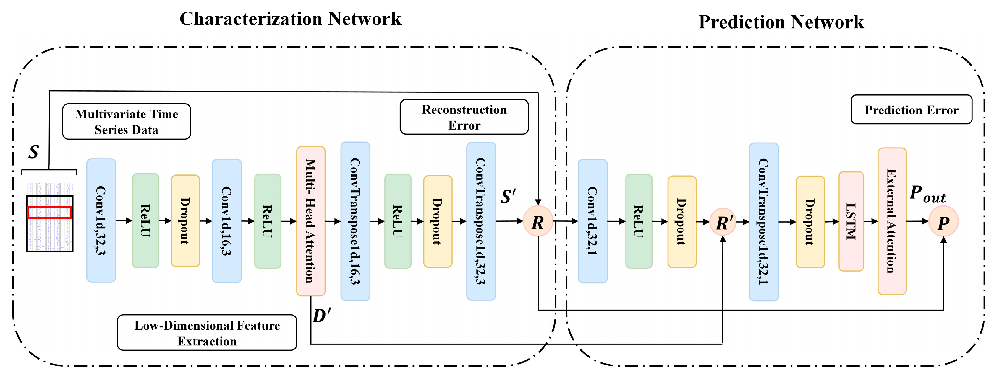
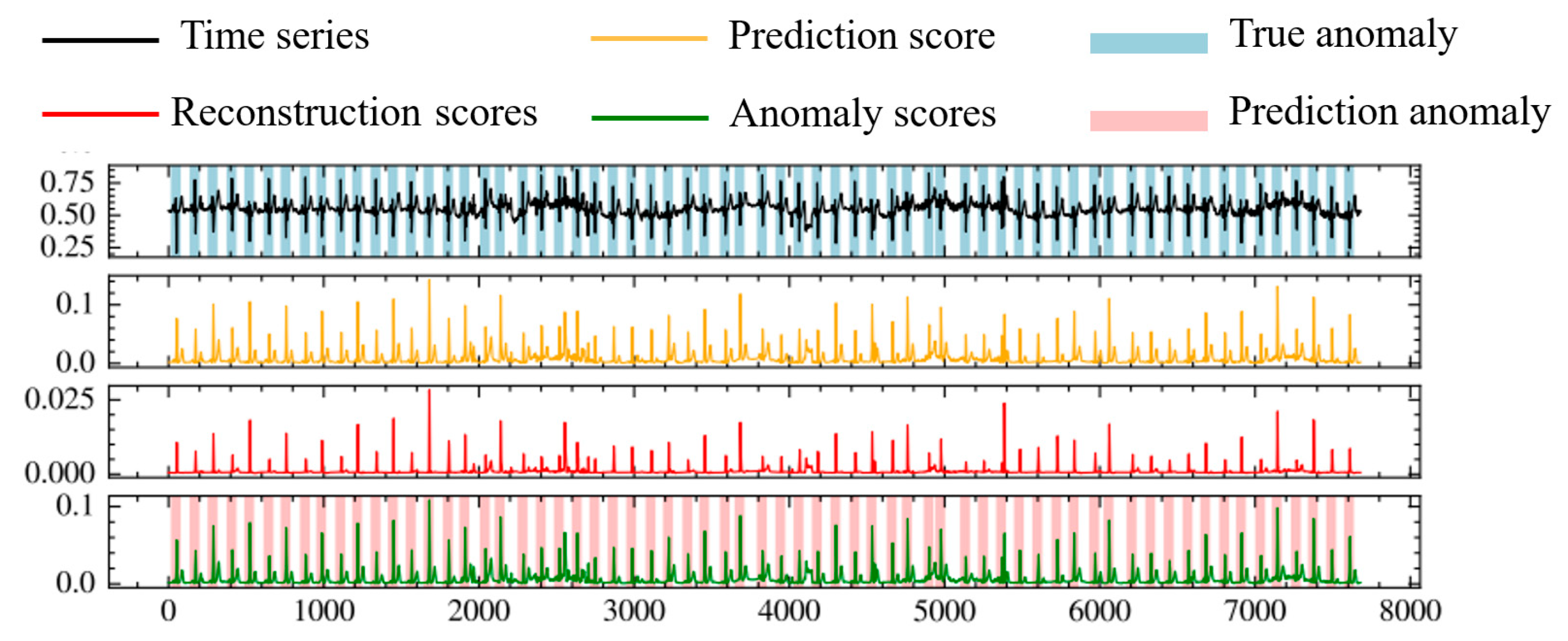
The model proposed in this paper mainly consists of two subnetworks. The first subnetwork is the characterization network, responsible for extracting low-dimensional spatial features from multivariate time-series data and calculating reconstruction errors. The second subnetwork is the prediction network, designed to capture time-dependent relationships. The characterization network encodes spatial information from multivariate time-series data into a low-dimensional representation. The incorporation of multi-head attention aims to focus on crucial information in the low-dimensional feature space. Subsequently, the characterization network calculates reconstruction errors. These reconstruction errors are then provided to the prediction network, which is based on an attention mechanism. The prediction network captures the temporal dependencies of the reconstruction errors from the characterization network and utilizes external attention to focus on important temporal information. Finally, both the characterization network and the prediction network undergo end-to-end training. For normal data, the reconstruction values generated by encoding the data are like the original input sequence, and the predicted values are like the future values of the time series. In contrast, for anomalous data, there is a significant deviation in both reconstruction and prediction values. Therefore, during the inference process, anomalies are precisely detected by calculating the anomaly score in the composite model.
We use the POT algorithm [29] to automatically calculate the anomaly threshold. When the anomaly score exceeds the threshold, we identify it as an anomalous event; otherwise, we consider it as a non-anomalous event. Figure 1 illustrates the proposed network architecture. In the figure, S represents the output of the characterization network, and R denotes the reconstruction error of the characterization network, computed as the square difference between the original input data S and S . R signifies the extracted low-dimensional key feature information D combined with the downsampled features of R . P represents the prediction error of the prediction network, calculated by subtracting P o u t from R .

3.4. Characterization Network

To better learn the spatial features of multivariate time-series data, we adopt a convolutional autoencoder structure suitable for handling anomaly detection in multivariate time-series data [
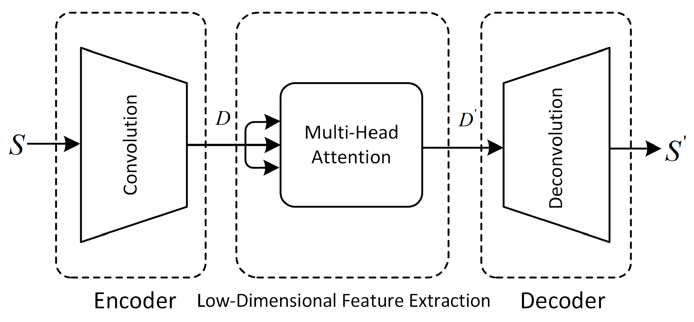
30]. This structure integrates CNN into the AutoEncode framework, where the convolutional kernel slides in the time dimension, extracting features at different time steps. By stacking multiple convolutional layers, higher-level time-series features are gradually extracted, learning the features and patterns of multivariate time-series data. The AutoEncode structure, through backpropagation and optimization methods like gradient descent, uses the input data itself as supervision to guide the neural network in attempting to learn a mapping relationship, resulting in a reconstructed output, achieving unsupervised training. The characterization network consists of three main parts: encoder, low-dimensional feature extraction, and decoder. The structure of the characterization network is illustrated in Figure 2.
The encoding process from the input layer to the hidden layer for the raw data S :
D = E n c o d e r ( S ) .
The process of extracting low-dimensional features:
D = M u l t i H e a d A t t ( D , D , D ) .
The decoding process from the hidden layer to the output layer:
S = D e c o d e r ( D ) .
The role of the encoder is to encode the high-dimensional input S into a low-dimensional latent variable D , enabling the neural network to learn the most informative features. The encoder achieves this by mapping the input S to the hidden representation D through two one-dimensional convolutional layers and one dropout layer. The addition of the dropout layer aims to enhance the network’s robustness, contributing to improved performance on noisy or highly variable data. The stride of each convolutional layer is set to 2, reducing the dimension of features and generating smaller-sized output feature maps based on the size of the convolutional kernel.
The intermediate hidden layer features encoded by the encoder, which represent the low-dimensional spatial feature information D , play a crucial role in identifying anomalies. Methods like CAE-M and DAGMM emphasize the significance of these features. To focus on the crucial information in the low-dimensional spatial features D , we introduce multi-head attention [30] into the low-dimensional space. Multi-head attention is capable of learning relationships between different low-dimensional features, combining various features to enhance the representation of the low-dimensional space, and capturing diverse dependencies within the low-dimensional space.
The calculation for each attention head d i ( i = 1 , , h ) in multi-head attention, given query q R d q , key k R d k , and value v R d v , is as follows:
d i = f W i q q , W i k k , W i v v R p v ,
W i q R p q × d q , W i k k R p k × d k , and W i v R p v × d v are learnable parameters. f represents the attention pooling function. The output of multi-head attention undergoes a linear transformation by concatenating multiple heads together and can be expressed as
W o d i R p v ,
where W o R p o × h p v is a learnable parameter. Based on this design, each head can focus on different parts of the low-dimensional features. Through this multi-head attention mechanism, the model can capture the intrinsic relationships within the low-dimensional spatial features. We have demonstrated the effectiveness of this approach through ablation experiments.
The role of the decoder is to map the crucial information from the low-dimensional spatial features D through reconstruction back to the original input space. Decoding involves transforming from a narrow representation to a wide reconstruction matrix, accomplished using transpose convolutional layers to increase width and height. The working principle of these layers is almost identical to convolutional layers but in reverse. We use the Rectified Linear Unit (ReLU) as the activation function for the convolutional layers.
During model training, only normal data are provided as training data, enabling the model to learn to reconstruct normal input data as accurately as possible. The ideal scenario is that the decoder’s output S can perfectly or approximately recover the original input S . The reconstructed values S , having the same structure as S , represent the reconstruction. The square of the difference between the original input data and their reconstruction is defined as the reconstruction error R . In this context, we utilize the Mean Squared Error (MSE) to measure the proximity between the original input and its reconstruction, as described by the following equation:
L r e c o n s t r u c t i o n   = S S 2

3.5. Prediction Network

To simultaneously capture the temporal and spatial dependencies of multivariate time series data, our proposed model characterizes the complex spatiotemporal patterns of multivariate time series data through both reconstruction analysis and prediction analysis. We use the reconstruction error of the characterization network as the original input R for the prediction network. A prediction network with a large reconstruction error will be more challenging to predict, resulting in a larger prediction error, while a prediction network with a smaller reconstruction error will be easier to predict, leading to a smaller prediction error.
The reconstruction error R is first fed into a one-dimensional convolutional layer with a stride of 4 and a kernel size of 1. The convolution operation downsamples the input sequence, reducing the number of time steps to one-fourth of the original. This helps reduce the computational cost of the model, improving training and inference efficiency. Using a kernel size of 1 in the convolutional layer is equivalent to performing independent linear transformations on the features of each time step. This aids the model in extracting and learning specific features for each time step without introducing a local perception field. Additionally, it allows for the reduction in the number of channels in the output of the convolutional layer while preserving input features. This helps compress the input data, making the model’s representation more compact and enhancing its ability to abstract input features. By aligning feature sizes, we merge the downsampled reconstruction loss with the low-dimensional feature information D extracted by the characterization network to obtain R . The purpose of this fusion is to introduce the low-dimensional feature representation learned by the characterization network into the features encoded after the reconstruction error. This fusion enables the network to comprehensively consider the information of the reconstruction loss and effectively handle it in the prediction network. In this way, a balance is achieved between the reconstruction error and the features learned by the characterization network to improve the overall performance and generalization ability of the entire network. Finally, R is upsampled to the original size to obtain the input E of the prediction function through a similar transpose convolution, as shown in the following equation:
D = D o w n s a m p l e ( R ) + D ,
E = U p s a m p l e ( D ) .
Prediction functions come in various types, such as the Recurrent Neural Network (RNN), Long Short-Term Memory (LSTM), and Gated Recurrent Unit (GRU) [31]. The original RNN struggles to learn long-term dependencies. In this work, we employ LSTM, a type of Recurrent Neural Network introduced by Hochreiter and Schmidhuber in 1997 [32]. Unlike conventional feedforward neural networks, LSTM networks can analyze input sequences over time. LSTM proves effective in transmitting and expressing information in long-time sequences, addressing the common issue of long-term dependencies being overlooked or forgotten in general recurrent neural networks. Additionally, LSTM resolves the problem of vanishing/exploding gradients present in RNNs. It employs a specialized architecture that integrates “gates” into the structure, consisting of four main components: forget gate f t , input gate i t , output gate o t , and a memory cell C t . e t represents the input at the t -th time step in E . The computation process for the hidden state h t is as follows:
f t = σ W f · h t 1 , e t + b f ,
i t = σ W i · h t 1 , e t + b i ,
o t = σ W o · h t 1 , e t + b o ,
C ~ t = t a n h W c h t 1 , e t + b c ,
C t = f t × C t 1 + i t × C ~ t ,
h t = o t × t a n h ( C t ) ,
Here, h t 1 , e t represents the horizontal concatenation of the hidden state h t 1 ; the input e t , σ ( ) and t a n h ( ) , respectively, represent the sigmoid and tanh activation functions; W g denotes weights; g stands for the gate neuron; b g is the bias of the gate; and h is the output of the previous LSTM cell. The LSTM forget gate, memory gate, and output gate control the information preservation and transmission in the LSTM, ultimately reflecting in the cell state C t and output signal h t . The key to LSTM is the cell state, which is like a conveyor belt running through the entire chain. The LSTM cell state allows the unit state to forget and replace values; then, it decides which values to output and sends them to the next unit. It controls the information passed to the next time step during the computation of the hidden state. It can consider global and local time information when calculating the hidden state.
To better handle time series data, we also introduce an attention mechanism, allowing the model to focus more on important information. Self-attention mechanisms [33] are widely used in computer vision [34], natural language processing [35], and other tasks due to their ability to capture long-term dependencies. However, self-attention mechanisms have a significant drawback: they require a considerable amount of computation, leading to some computational redundancy. Moreover, self-attention mechanisms only utilize information within their samples, neglecting potential connections between different samples.
To extract long-term dependencies in time series data and the potential connections between samples while reducing computational costs, we employ an external attention mechanism [36] using a small, learnable, and shared memory. External attention only uses two linear layers and normalization layers, possessing linear complexity and implicitly considering relationships between different feature maps.
External attention is achieved by introducing two external memory units, implicitly learning features of the entire dataset. It computes attention between the input and external memory units. The memory unit is represented as M R F × d , where F and d are hyperparameters. It can be expressed as
A = ( α ) i , j = N o r m ( O M T ) ,
P o u t = A M ,
where O represents the output of the LSTM at each time step in the input sequence and ( α ) i , j represents the similarity between the i -th element and the j -th row of M . The memory unit is a parameter independent of the input, serving as the memory for the entire training dataset.
In the output layer, the prediction error P is obtained by calculating the difference between the output P o u t of the prediction network and the true value R . The loss function of the prediction network can be expressed as
L p r e d i c t = R P o u t 2 .

3.6. Loss Function

We aim to minimize the loss function of AT-DCAEP, which consists of two parts: the reconstruction loss of the characterization network and the prediction loss of the prediction network. Our objective is to obtain better low-dimensional representation and reconstruction scores for multivariate time series data, along with crucial temporal information. The optimized loss function can be expressed as
L = S S 2 + R P o u t 2 ,
where S S 2 represents the reconstruction loss of the characterization network. A lower reconstruction loss indicates a good reconstruction of normal data. If the characterization network reconstruction is not good, the use of the prediction network to obtain prediction scores will be unreliable.
The term R P o u t 2 denotes the prediction loss of the prediction network. By minimizing the prediction loss, we ensure that the low-dimensional representation and reconstruction error in the characterization network accurately express key information for the current period. By minimizing both terms, we enable AT-DCAEP to effectively learn useful low-dimensional representation information for multivariate time series data, excelling in both reconstruction and capturing critical temporal information.

3.7. Inference

During the inference process, the reconstruction error is first obtained through the characterization network. Higher reconstruction scores are assigned to time steps with sudden changes in the time series. In the prediction network, greater attention is given to time series with larger deviations. The anomaly score is a linear combination of the reconstruction score and the prediction score, where α and β determine their relative influences, serving as tunable hyperparameters. The final expression for the a n o m a l y   s c o r e is as follows:
A n o m a l y   s c o r e = α S S 2 + β R P o u t 2 ,
After processing with the anomaly score function, the anomaly score for each sample is calculated. To ensure a fair comparison with other testing methods, we also use the POT (Peak Over Threshold) algorithm to select the threshold automatically and dynamically. Essentially, this is a statistical method that fits the data distribution to the generalized Pareto distribution using the “extreme value theory”. During the inference process, if the anomaly score is greater than the threshold automatically calculated by POT, the test sample is labeled as anomalous (1); otherwise, it is labeled as normal (0). Algorithm 1 outlines the complete training and inference process for AT-DCAEP.
Algorithm 1: Training and Inference procedure of AT-DCAEP
Training process
Input: Training dataset S
Output: Model parameter w
Randomly initialize parameter w ;
1: while not converge do
2:  Calculate low-dimensional representation D and reconstruction error R at each time step; //Equations (2) and (3)
3:  Apply downsampling to the reconstruction error R to get R ; //Equation (8)
4:  Add D and R and upsample to get E for each sample; //Equations (8) and (9)
5:  Predict the value P o u t using E by Attention-based LSTM model; //Equations (10)–(17)
6:  Update w by minimizing the compound objective function; //Equation (19)
7: return Optimal w ;
Inference process
Input: Testing dataset S ^ , model parameter w , hyperparameters α and β
Output: Label of all S ^ i
1: for all  S ^ i do
2:  Calculate the Anomaly Score; //Equation (20)
3:  Calculate the decision threshold THR by using POT;
4:  if Anomaly Score > THR then
5:     y i = 1 ;
6:  else
7:     y i = 0 ;
8: return Label of all S ^ i ;

4. Experiments

4.1. Datasets

We utilized six publicly available datasets in our experiments. Table 1 summarizes their characteristics, where (%) indicates the percentage of anomalous data points in the dataset.
  • Soil Moisture Active Passive (SMAP) Dataset: This dataset comprises soil samples and telemetry information from NASA’s Mars rover [37].
  • Secure Water Treatment (SWaT) Dataset: Originating from an actual water treatment plant, this dataset includes 11 days of continuous operation data, with 7 days of normal operation and 4 days of anomalous operation [38]. The dataset consists of sensor values (water level, flow, etc.) and actuator operations (valves and pumps).
  • Water Distribution (WADI) Dataset: An extension of the SWaT system, it has more than twice the number of sensors and actuators compared to the SWaT model [39]. The dataset spans 16 days, with 14 days of normal operation and 2 days of anomalous operation.
  • Server Machine Dataset (SMD): SMD is a newly released dataset collected by a large internet company over 5 weeks, containing monitoring data from 28 machines in a computing cluster [23]. SMD is divided into two equally sized subsets: the first half serves as the training set and the second half as the testing set.
  • Multi-Source Distributed System (MSDS) Dataset: This dataset comprises high-quality multi-source data, including distributed traces, application logs, and metrics from a complex distributed system [40]. Constructed specifically for artificial intelligence operations, it involves tasks such as automatic anomaly detection, root cause analysis, and remediation.
  • MIT-BIH Supraventricular Arrhythmia Database (MBA): Collected from four patients, this dataset includes electrocardiogram recordings with multiple instances of two different types of anomalies (atrial premature contractions or premature beats) [41,42]. It is a widely used, large-scale dataset in the data management community [43,44].
Table 1. Benchmarked datasets.
DatasetTrainTestDimensionsAnomalies (%)
MSDS146,430146,430105.37
SMD708,405708,420384.16
WADI1,048,571172,8011235.99
SWaT496,800449,9195111.98
SMAP135,183427,6172513.13
MBA100,000100,00020.14

4.2. Evaluation Metrics

We employ Precision ( P ), Recall ( R ), Receiver Operating Characteristic/Area Under the Curve ( R O C / A U C ), and F 1 score ( F 1 ) to assess the performance of anomaly detection:
P = T P T P + F P ,     R = T P T P + F N ,     F 1 = 2 P R P + R ,
where T P represents true positives, F P is false positives, and F N is false negatives. P and R signify precision and recall, respectively. A higher F 1 score indicates better performance. We partition 20% of the original testing dataset as the validation set and the remaining 80% as the testing set. After completing all model training, we measured the A U C and F 1 scores on the test dataset.

4.3. Results

We conducted comparative experiments with various baseline methods, including DAGMM [21], MAD-GAN [22], OmniAnomaly [23], CAE-M [24], MSCRED [25], USAD [26], GDN [27], TranAD [28], MERLIN [45], and MTAD-GAT [46]. We evaluated these methods on six different datasets, measuring their performance through comparisons of precision, recall, A U C , and F 1 scores. For a direct comparison with the benchmarks proposed by TranAD, we adopted their evaluation methodology.
As shown in Table 2, on average, the AT-DCAEP model achieved an average F 1 score of 0.9191 across the six datasets. While it performed slightly poorer on the SWaT dataset compared to other methods, it exhibited significantly superior F 1 scores on the remaining five datasets. Due to the longer sequence length and complex data patterns in the WADI dataset, all models showed relatively inferior performance on this dataset. However, our proposed approach demonstrated remarkable effectiveness on the WADI dataset compared to other methods. Specifically, the AT-DCAEP outperformed state-of-the-art baseline models with a 5.68% increase in the average F 1 score across the six datasets. These results indicate the significant advantages of the AT-DCAEP in multivariate time series anomaly detection tasks.

4.4. Hyperparameter Experiments

To explore the impact of the number of stacked convolutional layers (denoted as N) on the model’s performance, we experimented with different values of N. By comparing the model’s A U C and F 1 scores when N = 2 and N = 3, we observed that stacking more convolutional layers did not necessarily lead to better performance. The specific results are presented in Figure 3. In the case of N = 3, both A U C and F 1 scores showed a slight decrease across the six datasets. This suggests that increasing the number of convolutional layers does not always significantly improve model performance and may even have a negative impact.
We also conducted a study on the impact of the number of convolutional kernels on the effectiveness of anomaly detection. We configured different numbers of convolutional kernels to compare their performance in the model. Specifically, we designed three configurations with different numbers of convolutional kernels: the first layer of the convolutional encoder had 32 kernels and the second layer had 16 kernels (denoted as A T D C A E P A ); the first layer had 48 kernels and the second layer had 24 kernels (denoted as A T D C A E P B ); the first layer had 64 kernels and the second layer had 32 kernels (denoted as A T D C A E P C ). The convolutional decoder mirrored the hierarchical structure of the convolutional encoder. We compared the performance of these three configurations with different numbers of convolutional kernels, and the results are presented in Table 3. It is observed that, for the SWaT, SMD, and SMAP datasets, adopting a larger number of convolutional kernels did not enhance the performance of anomaly detection. In the MSDS, WADI, and MBA datasets, increasing the number of convolutional kernels even led to a decrease in performance. This indicates that augmenting the number of convolutional kernels does not always significantly improve performance; instead, it may increase computational costs. Therefore, careful consideration is required when choosing the stack depth of convolutional layers and the number of convolutional kernels, balancing performance and computational costs.
The adjustment of parameters α and β in the model is crucial, as they serve as tunable parameters with a significant impact on model effectiveness. A larger α corresponds to a stronger emphasis on the reconstruction contribution of the convolutional autoencoder in anomaly scoring, while a larger β corresponds to a greater emphasis on the contribution of prediction. Adjusting these parameters without retraining the model is essential for tuning detection sensitivity. Table 4 reports the impact of different α and β values on detection performance, including precision, recall, A U C , and F 1 scores.
It is observed that by increasing α and decreasing β , precision improved by 28.27% but recall decreased by 21.14%. The best A U C and F 1 scores were achieved at α = 0.3 and β = 0.7. Therefore, by adjusting α and β, the sensitivity of anomaly detection in the AT-DCAEP model can be parameterized to meet the requirements of real production environments. This tuning allows a single model to achieve different levels of sensitivity, catering to various needs in different layers of real production environments.

4.5. Visualizing Anomaly Results

Regarding the effectiveness of anomaly detection, taking the SMD 1-1 sensor dataset as an example, we illustrate the fluctuation of real values for variables 1 and 12 on the test set and their corresponding anomaly scores at each timestamp. Figure 4 indicates that the model performs well on the testing set, effectively expressing normal data. However, for anomalous data, the model struggles to represent them accurately, leading to higher anomaly scores.
To vividly showcase the effectiveness of our proposed anomaly detection method, we also visualize its performance on the MBA dataset. In Figure 5, subplots 1–4 and 5–8, respectively, display the real time series data, reconstruction scores, prediction scores, and anomaly scores for variables 1 and 2 in the MBA dataset. In Figure 6, subplots 1–4 present the real time series data, reconstruction scores, prediction scores, and anomaly scores. The blue area represents true anomaly regions, while the pink area indicates predicted anomaly regions. Anomalous behavior in one variable in multivariate time series data may trigger a series of events, leading to anomalies in other variables. The AT-DCAEP accurately localizes anomalous behavior to specific variables. As observed in the figure, our method accurately identifies most anomalous states in variables 1 and 2. Additionally, we find that combining reconstruction scores and prediction scores effectively enhances anomaly detection performance.
Through the visual presentation of anomaly detection results, the effectiveness of our method in multivariate time series data anomaly detection is clearly demonstrated, making a significant contribution to the advancement of the field.

5. Analysis

5.1. Ablation Study

To investigate the relative importance of each component in the model, we conducted ablation experiments, observing the change in model performance after removing each major component. The evaluation was based on A U C and F 1 scores. Specifically, we considered the following scenarios:
  • AT − DCAEPw/o Pre: removal of the prediction network, retaining only the characterization network for computing reconstruction error;
  • AT − DCAEPw/o LSTM: removal of the LSTM component from the prediction network;
  • AT − DCAEPw/o EAT: removal of the external attention component from the prediction network;
  • AT − DCAEPw/o LDFF: removal of low-dimensional feature fusion, i.e., no fusion of low-dimensional features extracted by the characterization network in the prediction network;
  • AT − DCAEPw/o MAT: removal of the multi-head attention module for low-dimensional feature extraction in the characterization network.
The experimental results are summarized in Table 5, indicating a corresponding performance decrease in F 1 scores when different components are removed. Specifically, the AT-DCAEP model without the prediction model experiences an average decrease of 5% in F 1 scores. This decrease is more pronounced in the WADI and MSDS datasets, with reductions of 8.5% and 12.7%, respectively, emphasizing the effectiveness and necessity of our composite model for anomaly detection in multivariate time series data.
Compared with the original AT-DCAEP model, removing the external attention component ( A T D C A E P w / o   E A T   ) results in a 7.6% decrease in the F 1 score for the WADI dataset and a 19% decrease for the MBA dataset, highlighting the critical role of external attention in the model. Similarly, removing the multi-head attention for low-dimensional feature extraction significantly reduces performance on most datasets, indicating the effectiveness of multi-head attention in capturing the relevance of low-dimensional features.

5.2. Overhead Analysis

The computational cost of the model is also a crucial evaluation criterion. An excellent algorithm for large-scale data should efficiently detect anomalies. To compare the computational cost and performance of these benchmark algorithms with our proposed method, we examined the time each model spent training for one epoch on different datasets. Additionally, we calculated the average training time and average F 1 score over the six datasets.
Figure 7 illustrates the computational cost and average F 1 score for each algorithm. Although our proposed method has a slightly higher average computational cost than TranAD, it is significantly lower than that of other methods. Moreover, our method achieves the highest average F 1 score, with an 8.79% improvement compared to TranAD.

5.3. Sensitivity Analysis

Figure 8 analyzes the sensitivity to training set size, showing the average F 1 scores and A U C scores on different datasets as the training data ratio varies. It also presents the change in training time as the training data ratio ranges from 20% to 100%. From the figure, it is evident that our proposed AT-DCAEP method achieves a significant performance improvement when the training dataset ratio reaches 60%. This strongly validates the excellence of our method in scenarios with small datasets. As the training data size increases, predictive performance shows an upward trend, accompanied by an increase in training time.
Additionally, we systematically tested the sensitivity of our proposed method to different window sizes, considering window sizes of [4,8,12,16,20,24]. As shown in Table 6, for the MSDS and SMAP datasets, the F 1 score and A U C achieved the best performance when the window size was 8, while for the MBA, WADI, and SMD datasets, the best F 1 score and A U C were obtained with a window size of 4. It is noteworthy that the SWaT dataset achieved the best F 1 score with a window size of 4, but the A U C was better with a window size of 8. Choosing a larger window size may enhance anomaly detection performance but could also increase computational costs. Conversely, smaller windows can detect behavioral changes more quickly but may miss longer-term anomalies.
Therefore, when selecting the window size, a balance between performance and computational costs is crucial. In real-world production environments, the choice of the most suitable window size should be based on specific needs and the context of the problem to achieve optimal anomaly detection performance.

6. Conclusions and Future Works

In this paper, we proposed the AT-DCAEP, a deep spatiotemporal network-based unsupervised anomaly detection method for multivariate time series data. The AT-DCAEP captures the spatiotemporal information of multivariate time series data through a convolutional autoencoder and extracts crucial information from the low-dimensional space using multi-head attention. This significantly improves the model’s reconstruction ability, particularly in reconstructing normal data, resulting in a substantial gain in reconstructing normal data. This characteristic enhances the model’s sensitivity to anomaly data, allowing for more accurate identification of anomalies. The prediction network based on external attention is then used to capture the temporal dependence of the reconstruction error. Finally, by simultaneously optimizing both subnetworks, the model’s anomaly detection performance is improved. We validated the effectiveness of this method on six different public datasets. Based on F 1 score performance, the AT-DCAEP surpassed the current state-of-the-art techniques in five out of six datasets, achieving a significant improvement in average F 1 score across all six datasets compared to the best baseline. The experimental results demonstrate that our proposed model is competitively robust in the field of anomaly detection and has broad application prospects.
However, despite these advancements, the proposed model exhibits limitations in coupling spatiotemporal features, as the predictive network solely analyzes reconstruction errors, overlooking global trend analysis. If the performance of the reconstruction network is subpar, it may significantly impact the accuracy of the predictive network, and its independence needs enhancement. In the future, we will focus on researching more effective multivariate time series anomaly detection methods to address these limitations, exploring approaches for spatiotemporal feature coupling to enhance the model’s adaptability and robustness. Additionally, we plan to investigate anomaly detection methods suitable for edge devices with limited computational capabilities. By deploying the model on edge intelligent devices, we aim to achieve real-time online monitoring of anomalies, which holds significant implications for advancing Industry 4.0.

Author Contributions

Conceptualization, P.L. and R.T.; methodology, W.L. and N.M.; resources, R.T. and P.L.; data curation, G.W. and L.Y.; investigation, X.M.; validation, G.W., L.Y. and X.M.; writing—original draft preparation, W.L.; writing—review and editing, P.L., W.L. and N.M.; and supervision, P.L. All authors have read and agreed to the published version of the manuscript.

Funding

This research was funded by the National Key Research and Development Program of China, grant number 2022YFB3305300, and supported by State Grid Shandong Electric Power Company Technology Project (No. 520627230004). The authors declare that this study received funding from State Grid Shandong Electric Power Company. The funder had the following involvement with the study: data curation and validation.

Data Availability Statement

Publicly available datasets were analyzed in this study. This data can be found here: https://github.com/imperial-qore/TranAD/tree/main/data (accessed on 16 December 2023). Restrictions apply to the availability of WADI dataset. Data was obtained from iTRUST and is available at https://itrust.sutd.edu.sg/itrust-labs_datasets/dataset_info/#wadi (accessed on 16 October 2023) with the permission of iTRUST.

Conflicts of Interest

Authors Li Yan and Gaozhou Wang were employed by Information and Telecommunication Company, State Grid Shandong Electric Power Company. The remaining authors declare that the research was conducted in the absence of any commercial or financial rela-tionships that could be construed as a potential conflict of interest. The authors declare that this study received funding from State Grid Shandong Electric Power Company. The funder had the following involvement with the study: data curation and validation.

References

  1. Raut, R.D.; Gotmare, A.; Narkhede, B.E.; Govindarajan, U.H.; Bokade, S.U. Enabling technologies for Industry 4.0 manufacturing and supply chain: Concepts, current status, and adoption challenges. IEEE Eng. Manag. Rev. 2020, 48, 83–102. [Google Scholar] [CrossRef]
  2. Patel, P.; Ali, M.I.; Sheth, A. From raw data to smart manufacturing: AI and semantic web of things for industry 4.0. IEEE Intell. Syst. 2018, 33, 79–86. [Google Scholar] [CrossRef]
  3. Liang, W.; Huang, W.; Long, J.; Zhang, K.; Li, K.-C.; Zhang, D. Deep reinforcement learning for resource protection and real-time detection in IoT environment. IEEE Internet Things J. 2020, 7, 6392–6401. [Google Scholar] [CrossRef]
  4. Cai, Z.; He, Z. Trading private range counting over big IoT data. In Proceedings of the 2019 IEEE 39th International Conference on Distributed Computing Systems (ICDCS), Dallas, TX, USA, 7–9 July 2019; pp. 144–153. [Google Scholar]
  5. Demertzis, K.; Iliadis, L.; Tziritas, N.; Kikiras, P. Anomaly detection via blockchained deep learning smart contracts in industry 4.0. Neural Comput. Appl. 2020, 32, 17361–17378. [Google Scholar] [CrossRef]
  6. Kong, F.; Li, J.; Jiang, B.; Wang, H.; Song, H. Integrated generative model for industrial anomaly detection via Bidirectional LSTM and attention mechanism. IEEE Trans. Ind. Inform. 2023, 19, 541–550. [Google Scholar] [CrossRef]
  7. Gupta, M.; Gao, J.; Aggarwal, C.C.; Han, J. Outlier detection for temporal data: A survey. IEEE Trans. Knowl. Data Eng. 2013, 26, 2250–2267. [Google Scholar] [CrossRef]
  8. Choi, K.; Yi, J.; Park, C.; Yoon, S. Deep learning for anomaly detection in time-series data: Review, analysis, and guidelines. IEEE Access 2021, 9, 120043–120065. [Google Scholar] [CrossRef]
  9. Markou, M.; Singh, S. Novelty detection: A review—Part 1: Statistical approaches. Signal Process. 2003, 83, 2481–2497. [Google Scholar] [CrossRef]
  10. Kiss, I.; Genge, B.; Haller, P.; Sebestyén, G. Data clustering-based anomaly detection in industrial control systems. In Proceedings of the 2014 IEEE 10th International Conference on Intelligent Computer Communication and Processing (ICCP), Cluj-Napoca, Romania, 4–6 September 2014; pp. 275–281. [Google Scholar]
  11. Ma, J.; Perkins, S. Time-series novelty detection using one-class support vector machines. In Proceedings of the International Joint Conference on Neural Networks, Portland, OR, USA, 20–24 July 2003; pp. 1741–1745. [Google Scholar]
  12. Chaovalitwongse, W.A.; Fan, Y.-J.; Sachdeo, R.C. On the time series k-nearest neighbor classification of abnormal brain activity. IEEE Trans. Syst. Man Cybern. Paart A-Syst. Hum. 2007, 37, 1005–1016. [Google Scholar] [CrossRef]
  13. Liu, F.T.; Ting, K.M.; Zhou, Z.-H. Isolation forest. In Proceedings of the 2008 Eighth IEEE International Conference on Data Mining, Pisa, Italy, 15–19 December 2008; pp. 413–422. [Google Scholar]
  14. Shipmon, D.T.; Gurevitch, J.M.; Piselli, P.M.; Edwards, S.T. Time series anomaly detection; detection of anomalous drops with limited features and sparse examples in noisy highly periodic data. arXiv 2017, arXiv:abs/1708.03665. [Google Scholar]
  15. Chen, J.; Sathe, S.; Aggarwal, C.; Turaga, D. Outlier detection with autoencoder ensembles. In Proceedings of the 2017 SIAM International Conference on Data Mining, Houston, TX, USA, 27–29 April 2017; pp. 90–98. [Google Scholar]
  16. Chen, H.; Liu, H.; Chu, X.; Liu, Q.; Xue, D. Anomaly detection and critical SCADA parameters identification for wind turbines based on LSTM-AE neural network. Renew. Energy 2021, 172, 829–840. [Google Scholar] [CrossRef]
  17. Park, D.; Hoshi, Y.; Kemp, C.C. A multimodal anomaly detector for robot-assisted feeding using an lstm-based variational autoencoder. IEEE Robot. Autom. Lett. 2018, 3, 1544–1551. [Google Scholar] [CrossRef]
  18. Shi, X.; Chen, Z.; Wang, H.; Yeung, D.-Y.; Wong, W.-k.; Woo, W.-c. Convolutional LSTM Network: A machine learning approach for precipitation nowcasting. In Proceedings of the 28th International Conference on Neural Information Processing Systems—Volume 1, Montreal, QC, Canada; 2015; pp. 802–810. [Google Scholar]
  19. Kim, T.-Y.; Cho, S.-B. Web traffic anomaly detection using C-LSTM neural networks. Expert Syst. Appl. 2018, 106, 66–76. [Google Scholar] [CrossRef]
  20. Kim, Y.; Moschitti, A.; Pang, B.; Daelemans, W. Convolutional neural networks for sentence classification. In Proceedings of the 2014 Conference on Empirical Methods in Natural Language Processing (EMNLP), Doha, Qatar, 25–29 October 2014; pp. 1746–1751. [Google Scholar]
  21. Zong, B.; Song, Q.; Min, M.R.; Cheng, W.; Lumezanu, C.; Cho, D.; Chen, H. Deep autoencoding gaussian mixture model for unsupervised anomaly detection. In Proceedings of the International Conference on Learning Representations, Vancouver, BC, Canada, 30 April–3 May 2018. [Google Scholar]
  22. Li, D.; Chen, D.; Jin, B.; Shi, L.; Goh, J.; Ng, S.-K. MAD-GAN: Multivariate anomaly detection for time series data with generative adversarial networks. In Proceedings of the International Conference on Artificial Neural Networks, Munich, Germany, 17–19 September 2019; pp. 703–716. [Google Scholar]
  23. Su, Y.; Zhao, Y.; Niu, C.; Liu, R.; Sun, W.; Pei, D. Robust anomaly detection for multivariate time series through stochastic recurrent neural network. In Proceedings of the 25th ACM SIGKDD International Conference on Knowledge Discovery & Data Mining, Anchorage, AK, USA, 4–8 August 2019; pp. 2828–2837. [Google Scholar]
  24. Zhang, Y.; Chen, Y.; Wang, J.; Pan, Z. Unsupervised deep anomaly detection for multi-sensor time-series signals. IEEE Trans. Knowl. Data Eng. 2023, 35, 2118–2132. [Google Scholar] [CrossRef]
  25. Zhang, C.; Song, D.; Chen, Y.; Feng, X.; Lumezanu, C.; Cheng, W.; Ni, J.; Zong, B.; Chen, H.; Chawla, N.V. A deep neural network for unsupervised anomaly detection and diagnosis in multivariate time series data. In Proceedings of the AAAI Conference on Artificial Intelligence, Honolulu, HI, USA, 27 January–1 February 2019; pp. 1409–1416. [Google Scholar]
  26. Audibert, J.; Michiardi, P.; Guyard, F.; Marti, S.; Zuluaga, M.A. Usad: Unsupervised anomaly detection on multivariate time series. In Proceedings of the 26th ACM SIGKDD International Conference on Knowledge Discovery & Data Mining, Online, 6–10 July 2020; pp. 3395–3404. [Google Scholar]
  27. Deng, A.; Hooi, B. Graph neural network-based anomaly detection in multivariate time series. In Proceedings of the AAAI Conference on Artificial Intelligence, Online, 2–9 February 2021; pp. 4027–4035. [Google Scholar]
  28. Tuli, S.; Casale, G.; Jennings, N.R. Tranad: Deep transformer networks for anomaly detection in multivariate time series data. Proc. VLDB Endow. 2022, 15, 1201–1214. [Google Scholar] [CrossRef]
  29. Siffer, A.; Fouque, P.-A.; Termier, A.; Largouet, C. Anomaly detection in streams with extreme value theory. In Proceedings of the 23rd ACM SIGKDD International Conference on Knowledge Discovery and Data Mining, Halifax, NS, Canada, 13–17 August 2017; pp. 1067–1075. [Google Scholar]
  30. Francois, C. Building Autoencoders in Keras. Available online: https://blog.keras.io/building-autoencoders-in-keras.html (accessed on 7 December 2023).
  31. Chung, J.; Gulcehre, C.; Cho, K.; Bengio, Y. Empirical evaluation of gated recurrent neural networks on sequence modeling. arXiv 2014, arXiv:abs/1412.3555. [Google Scholar]
  32. Hochreiter, S.; Schmidhuber, J. Long Short-Term Memory. Neural Comput. 1997, 9, 1735–1780. [Google Scholar] [CrossRef]
  33. Vaswani, A.; Shazeer, N.; Parmar, N.; Uszkoreit, J.; Jones, L.; Gomez, A.N.; Kaiser, Ł.; Polosukhin, I. Attention is all you need. In Proceedings of the 31st International Conference on Neural Information Processing Systems, Long Beach, CA, USA, 4–9 December 2017; pp. 6000–6010. [Google Scholar]
  34. Wang, X.; Girshick, R.; Gupta, A.; He, K. Non-local neural networks. In Proceedings of the IEEE Conference on Computer Vision and Pattern Recognition, Salt Lake City, UT, USA, 18–23 June 2018; pp. 7794–7803. [Google Scholar]
  35. Tan, Z.; Wang, M.; Xie, J.; Chen, Y.; Shi, X. Deep semantic role labeling with self-attention. In Proceedings of the AAAI Conference on Artificial Intelligence, New Orleans, LA, USA, 2–7 February 2018; pp. 4929–4936. [Google Scholar]
  36. Guo, M.-H.; Liu, Z.-N.; Mu, T.-J.; Hu, S.-M. Beyond self-attention: External attention using two linear layers for visual tasks. IEEE Trans. Pattern Anal. Mach. Intell. 2022, 45, 5436–5447. [Google Scholar] [CrossRef] [PubMed]
  37. Hundman, K.; Constantinou, V.; Laporte, C.; Colwell, I.; Soderstrom, T. Detecting spacecraft anomalies using lstms and nonparametric dynamic thresholding. In Proceedings of the 24th ACM SIGKDD International Conference on Knowledge Discovery & Data Mining, London, UK, 19–23 August 2018; pp. 387–395. [Google Scholar]
  38. Mathur, A.P.; Tippenhauer, N.O. SWaT: A water treatment testbed for research and training on ICS security. In Proceedings of the 2016 International Workshop on Cyber-Physical Systems for Smart Water Networks (CySWater), Vienna, Austria, 11 April 2016; pp. 31–36. [Google Scholar]
  39. Ahmed, C.M.; Palleti, V.R.; Mathur, A.P. WADI: A water distribution testbed for research in the design of secure cyber physical systems. In Proceedings of the 3rd International Workshop on Cyber-Physical Systems for Smart Water Networks, Pittsburgh, PA, USA, 21 April 2017; pp. 25–28. [Google Scholar]
  40. Nedelkoski, S.; Bogatinovski, J.; Mandapati, A.K.; Becker, S.; Cardoso, J.; Kao, O. Multi-source distributed system data for ai-powered analytics. In Proceedings of the Service-Oriented and Cloud Computing: 8th IFIP WG 2.14 European Conference (ESOCC 2020), Heraklion, Greece, 28–30 September 2020; pp. 161–176. [Google Scholar]
  41. Goldberger, A.L.; Amaral, L.A.; Glass, L.; Hausdorff, J.M.; Ivanov, P.C.; Mark, R.G.; Mietus, J.E.; Moody, G.B.; Peng, C.-K.; Stanley, H.E. PhysioBank, PhysioToolkit, and PhysioNet: Components of a new research resource for complex physiologic signals. Circulation 2000, 101, e215–e220. [Google Scholar] [CrossRef] [PubMed]
  42. Moody, G.B.; Mark, R.G. The impact of the MIT-BIH arrhythmia database. IEEE Eng. Med. Biol. Mag. 2001, 20, 45–50. [Google Scholar] [CrossRef]
  43. Boniol, P.; Linardi, M.; Roncallo, F.; Palpanas, T. Automated anomaly detection in large sequences. In Proceedings of the 2020 IEEE 36th International Conference on Data Engineering (ICDE), Dallas, TX, USA, 20–24 April 2020; pp. 1834–1837. [Google Scholar]
  44. Boniol, P.; Paparrizos, J.; Palpanas, T.; Franklin, M.J. SAND: Streaming subsequence anomaly detection. Proc. VLDB Endow. 2021, 14, 1717–1729. [Google Scholar] [CrossRef]
  45. Nakamura, T.; Imamura, M.; Mercer, R.; Keogh, E. Merlin: Parameter-free discovery of arbitrary length anomalies in massive time series archives. In Proceedings of the 2020 IEEE International Conference on Data Mining (ICDM), Sorrento, Italy, 17–20 November 2020; pp. 1190–1195. [Google Scholar]
  46. Zhao, H.; Wang, Y.; Duan, J.; Huang, C.; Cao, D.; Tong, Y.; Xu, B.; Bai, J.; Tong, J.; Zhang, Q. Multivariate time-series anomaly detection via graph attention network. In Proceedings of the 2020 IEEE International Conference on Data Mining (ICDM), Sorrento, Italy, 17–20 November 2020; pp. 841–850. [Google Scholar]
Figure 1. The architecture of the AT-DCAEP model.
Applsci 14 00774 g001
Figure 2. Characterization network structure diagram.
Applsci 14 00774 g002
Figure 3. Impact of the number of convolutional layers on model performance. (a) The impact of the number of convolutional layers on AUC. (b) The impact of the number of convolutional layers on F1 score.
Applsci 14 00774 g003
Figure 4. Visualization of the AT-DCAEP model on the SMD dataset.
Applsci 14 00774 g004
Figure 5. Variable-wise visualization on MBA dataset.
Applsci 14 00774 g005
Figure 6. Comprehensive visualization on MBA dataset.
Applsci 14 00774 g006
Figure 7. Average time cost (minutes) and average F1 score analysis.
Applsci 14 00774 g007
Figure 8. Sensitivity analysis of training set size.
Applsci 14 00774 g008
Table 2. Performance comparison of AT-DCAEP with baseline methods. P: Precision, R: Recall, AUC: Area Under the ROC Curve, F1: F1 score on the entire training dataset. The best F1 and AUC scores are highlighted in bold.
MethodMBASMAPSMD
P R A U C F1 P R A U C F1 P R A U C F1
DAGMM0.94750.99990.98580.97300.80690.99990.98840.89310.94020.99730.99540.9679
OmniAnomaly0.85950.99990.95810.92440.79910.99990.98780.88830.98840.99850.99860.9934
MERLIN0.98460.04920.52440.09370.15770.99990.74260.27250.28490.56280.70840.3783
MSCRED0.92490.99990.97920.96100.81750.92160.98210.86640.72760.99740.99210.8414
MAD-GAN0.93960.99990.98350.96880.81570.99990.98910.89840.99990.40230.70110.5737
USAD0.89530.99990.97000.94470.81390.99990.98890.89740.90690.99730.99330.9499
MTAD-GAT0.98970.98970.99730.99480.75170.99990.98400.85820.82100.92150.99210.8683
CAE-M0.87890.99990.96470.93550.83950.99990.99070.91270.69540.99730.99330.9499
GDN0.84410.99990.95270.91540.94760.41170.70470.57400.71690.99730.97830.8342
TranAD0.95690.99990.98840.97790.80430.99990.98820.89150.90720.99730.99340.9501
AT-DCAEP0.99230.99990.99800.99610.89040.99990.99400.94200.9940.99810.99870.9960
MethodSWaTWADIMSDS
P R A U C F1 P R A U C F1 P R A U C F1
DAGMM0.99320.68780.84350.81280.49400.82950.90470.61920.99990.81250.90620.8965
OmniAnomaly0.97600.69560.84650.81230.78370.65410.82490.71311.00000.79640.89820.8867
MERLIN0.65590.25460.61740.36680.06350.76690.74990.11740.72540.31100.50220.4353
MSCRED0.99990.67700.83850.80740.25130.73190.84120.37411.00000.79830.89430.8878
MAD-GAN0.95930.69560.84560.80640.22330.91240.80260.35880.81570.92160.98910.8654
USAD0.99770.68780.84380.81430.19890.82950.87530.32080.74800.96270.98900.8419
MTAD-GAT0.97600.69560.84650.81230.28180.80120.88210.41690.99970.88880.94410.9410
CAE-M0.95930.69560.84560.80640.27820.79180.87280.41170.99990.88150.94070.9370
GDN0.96960.69560.84620.81010.29120.79310.87770.42600.97260.86060.89880.9132
TranAD0.99770.68780.84380.81430.39920.82950.90000.53900.99990.81250.90620.8965
AT-DCAEP0.99770.67700.83830.80660.78800.82950.91210.80820.99240.94060.96090.9658
Table 3. Impact of the number of convolutional kernels on performance.
Method A T D C A E P A A T D C A E P B A T D C A E P C
P R A U C F 1 P R A U C F 1 P R A U C F 1
MSDS0.99240.94060.96090.96580.88810.99560.83440.93870.84000.99830.75160.9123
SWaT0.99770.67700.83830.80660.99770.67700.83830.80660.99770.67700.83830.8066
SMD0.99400.99810.99870.99600.99400.99810.99870.99600.99400.99810.99870.9960
WADI0.78800.82950.91210.80820.74210.82950.91130.78340.74380.82950.91140.7843
SMAP0.89040.99990.99400.94200.89040.99990.99400.94200.88830.99990.99390.9408
MBA0.99230.99990.99800.99610.98700.99990.99660.99340.99000.99990.99740.9950
Table 4. Anomaly detection results on the WADI dataset based on different sensitivities.
α β P R A U C F 1
0.10.90.69680.82950.91050.7574
0.20.80.76600.82950.91170.7966
0.30.70.78800.82950.91210.8082
0.40.60.77910.65410.82480.7111
0.50.50.79810.65410.82510.7190
0.60.40.82330.65410.82540.7290
0.70.30.85850.65410.82570.7425
0.80.20.87580.65410.82590.7489
0.90.10.89380.65410.82610.7554
Table 5. Ablation study of AT-DCAEP and its ablated versions with AUC and F1 scores.
MethodWADIMSDSMBA
A U C F1 A U C F1 A U C F1
A T D C A E P w / o   P r e   0.82570.73930.51630.84330.95450.9183
A T D C A E P w / o   L S T M   0.82570.74250.95770.96130.99780.9957
A T D C A E P w / o   E A T   0.82590.74670.95910.96300.83830.8066
A T D C A E P w / o   L D F F   0.91200.80630.95770.96130.99790.9959
A T D C A E P w / o   M A T   0.91050.75740.74610.91060.97080.9461
A T D C A E P 0.91210.80820.96090.96580.99800.9961
MethodSMAPSMDSWaT
A U C F1 A U C F1 A U C F1
A T D C A E P w / o   P r e   0.99330.93550.99820.99450.84250.8061
A T D C A E P w / o   L S T M   0.99390.94080.99830.99560.84240.8054
A T D C A E P w / o   E A T   0.99380.93960.99830.99560.84510.8035
A T D C A E P w / o   L D F F   0.99380.94020.99830.99560.84230.8047
A T D C A E P w / o   M A T   0.99380.94020.99820.99420.84230.8047
A T D C A E P 0.99400.94200.99870.99600.83830.8066
Table 6. Impact of window size parameter on performance.
Size A U C F 1
MSDSMBASMAPSWaTWADISMDMSDSMBASMAPSWaTWADISMD
40.81290.99800.83730.83830.91210.99870.93180.99610.78690.80660.80820.9960
80.96090.98240.99400.84230.90900.99830.96580.97330.94200.80470.71560.9956
120.90040.95700.99340.84090.90640.99790.88950.93330.93610.79600.65540.9806
160.90040.93780.99240.83870.90000.99770.88950.90560.92740.78260.53990.9787
200.90030.90700.69730.83910.88820.99720.88940.85300.51800.78470.40710.9742
240.90030.86060.69620.83590.87030.99750.88940.78790.51110.76570.29690.9767
Disclaimer/Publisher’s Note: The statements, opinions and data contained in all publications are solely those of the individual author(s) and contributor(s) and not of MDPI and/or the editor(s). MDPI and/or the editor(s) disclaim responsibility for any injury to people or property resulting from any ideas, methods, instructions or products referred to in the content.

